Pattern Selection in a Phase Field Model for Directional Solidification

Abstract

A symmetric phase field model is used to study wavelength selection in two dimensions. We study the problem in a finite system using a two-pronged approach. First we construct an action and, minimizing this, we obtain the most probable configuration of the system, which we identify with the selected stationary state. The minimization is constrained by the stationary solutions of stochastic evolution equations and is done numerically. Secondly, additional support for this selected state is obtained from straightforward simulations of the dynamics from a variety of initial states.

I Introduction

The problem of pattern selection is to predict which pattern, out of a number of possible stationary patterns, will be selected under given experimental conditions. This problem has been of great interest for many years in many fields such as biology, chemistry, engineering and physics CrossHohenberg where a large variety of reproducible patterns can be formed under various external conditions which drive the system away from thermal and mechanical equilibrium. Important examples of pattern selection are directional solidification and eutectic growth where the interface between the ordered and disordered phases can take a periodic cellular pattern. From the experimental point of view, the interface seems to have a well defined periodicity in both directed one phase solidification bechhoefer87 ; billia87 ; flesselles91 and in directed eutectic solidification jacksonhunt66 ; ginibre97 . On the theoretical side, there is much disagreement with some researchers claiming that a unique wavelength is selected karma86 ; kerszberg1 ; kerszberg2 ; kerszberg3 ; kurtze96 while others say that the wavelength of the final pattern is accidental dombre87 ; amar88 . A large scale simulation on a noisy Swift Hohenberg equation swifthohenberg which models fluid convection near onset has been done garcia93 to study the selection of periodic patterns. For this system, a potential ${\cal F}_{SH}$ exists and minimizing this gives the unique selected stationary pattern for any initial state, exactly as for a system approaching equilibrium.

In this paper, we use a numerical and a theoretical approach to argue that in the presence of noise, there is a wavelength selection for the cellular pattern formation in the directional solidification problem, see Fig. 1. More precisely, we use a phase field model with additive stochastic noise developed for growth processes such as single phase directional solidification driven out of equilibrium by an external moving temperature gradient grossmann93 ; drolet94 ; drolet00 . This causes invasion of a disordered by an ordered phase with non potential dynamics. Since we are unable to solve the problem analytically, we use numerical computations which limit us to rather small system sizes. However, we believe that this is sufficient to demonstrate our conjecture of a unique selected state. In addition, we construct an action and, minimizing this, we obtain the most probable configuration of the system, which we identify with the selected stationary state. The minimization is constrained by the stationary solutions of stochastic evolution equations which are calculated numerically.

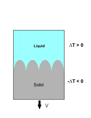
Figure 1: A schematic representation of the cellular pattern in directional solidification. $\Delta T=(T-T_{m})/T_{m}$ where $T_{m}$ is the melting temperature of the pure solid.

II Phase-field model

To carry out our simulations, we use a phase-field model for directional solidification based on two continuum fields to describe the phases of the system. These fields vary slowly in the bulk region and rapidly near the solid-liquid interface. The equilibrium system is described by a free energy functional ${\cal F}(c,\psi)$ grossmann93 where

$${\cal F}(c,\psi) = \int d{\bf r}\left[\frac{K_{\psi}}{2}(\nabla\psi)^{2}+\frac{K_{c}}{2}(\nabla c)^{2}+f(c,\psi)\right]$$ (1)

$$f(c,\psi) = -\frac{1}{2}\psi^{2}+\frac{1}{4}\psi^{4}+\Delta Th(\psi)+\frac{1}{2}\gamma\Delta\psi\left(c+\frac{h(\psi)}{\Delta\psi}\right)^{2}$$ (2)

$$h(\psi) = \frac{15}{8}\left(\psi-\frac{2}{3}\psi^{3}+\frac{1}{5}\psi^{5}\right).$$ (3)

Here, $\psi$ is a nonconserved order parameter field which has one value in the solid and another in the liquid and c is a dimensionless diffusion field proportional to the impurity concentration. $\Delta T=(T-T_{m})/T_{m}$ where $T_{m}$ is the melting temperature of the pure solid when $c=0$. $\Delta\psi$ is the discontinuity in $\psi$ between solid and liquid, $K_{\psi}$ and $K_{c}$ are phenomenological constants accounting for the free energy cost of spatial variations in $\psi$ and $c$. The Kobayashi function, $h(\psi)$ kobayashi93 , is introduced for analytic and computational convenience to simplify the problem, despite the apparent additional complexity karma98 ; egpk01 . It has essentially the same effect as $\psi$ itself as $h(\psi)$ is chosen to have the properties (i) $h(\pm 1)=\pm 1$ and (ii) $\delta h/\delta\psi=0$ when $\psi=\pm 1$. This choice ensures that the equilibrium values of $\psi$ are $\psi_{eq}=+1$ for $\Delta T>0$ and $\psi_{eq}=-1$ for $\Delta T<0$ independently of the values of $\Delta T$ and $c$ so that $\Delta\psi=2$. The interface between the ordered $\Delta T<0$ and the disordered $\Delta T>0$ phases is the region over which the fields $\psi$ and $c$ change from one bulk value to the other and has a width $\xi={\cal O}(1)$, we define its position $(x,z)$ by $\psi(x,z)=0$.

To impose the motion of the interface, we take $\Delta T({\bf r},t)=\Delta T(z-vt)$ where ${\bf v}=v{\bf\hat{z}}$ is the externally imposed pulling velocity. Stationary states can exist only in the frame moving with the interface when $\Delta T({\bf r},t)=\Delta T(z)$. In this frame, the simplest possible dynamics consistent with the macroscopic conservation law for $c$ are Langevin equations hohenberghalperin

$$\dot{\psi}=\frac{\partial\psi}{\partial t} = -\Gamma_{\psi}\frac{\delta{\cal F}}{\delta\psi}+v\frac{\partial\psi}{\partial z}+\eta_{\psi}\equiv{\cal G}_{\psi}+\eta_{\psi}$$ (4)

$$\dot{c}=\frac{\partial c}{\partial t} = \Gamma_{c}{\bf\nabla}^{2}\frac{\delta{\cal F}}{\delta c}+v\frac{\partial c}{\partial z}+\eta_{c}\equiv{\cal G}_{c}+\eta_{c}$$ (5)

where $\Gamma_{\psi}$ and $\Gamma_{c}$ are the mobilities of the fields $\psi$ and $c$ respectively. Complications such as fluid flow are not considered. Note that the non dissipative terms $v\partial\psi/\partial z$ and $v\partial c/\partial z$ cannot be written as derivatives of a potential so that the dynamics of Eq. (4) is non potential. This makes the construction of a differentiable Lyapunov functional for such situations difficult but such a procedure has been implemented successfully in a similar situation graham90 ; montagne96 . The stochastic noises $\eta_{\psi}({\bf r},t)$ and $\eta_{c}({\bf r},t)$ have probability distributions

$${\cal P}(\eta_{c}) \propto{\rm exp}\Bigl{[}-\frac{1}{4\Gamma^{\prime}_{c}}\int dtd{\bf r}d{\bf r^{\prime}}\eta_{c}({\bf r},t)G({\bf r},{\bf r^{\prime}})\eta_{c}({\bf r^{\prime}},t)\Bigr{]}$$ (6)

$${\cal P}(\eta_{\psi}) \propto{\rm exp}\Bigl{[}-\frac{1}{4\Gamma^{\prime}_{\psi}}\int dtd{\bf r}(\eta_{\psi}({\bf r},t))^{2}\Bigr{]}$$ (7)

When $v=0$ in Eq. (4) the system approaches its stationary equilibrium state given by the minimum of ${\cal F}(c,\psi)$ graham90 ; hohenberghalperin . $G({\bf r},{\bf r^{\prime}})$ obeys $\nabla^{2}G({\bf r},{\bf r^{\prime}})=-\delta({\bf r}-{\bf r^{\prime}})$ with appropriate boundary conditions and $G^{-1}({\bf r},{\bf r^{\prime}})=-\nabla^{2}\delta({\bf r}-{\bf r^{\prime}})$ so

$$\langle\eta_{\psi}({\bf r},t)\eta_{\psi}({\bf r^{\prime}},t^{\prime})\rangle = 2\Gamma^{\prime}_{\psi}\delta({\bf r}-{\bf r^{\prime}})\delta(t-t^{\prime})$$ (8)

$$\langle\eta_{c}({\bf r},t)\eta_{c}({\bf r^{\prime}},t^{\prime})\rangle = 2\Gamma^{\prime}_{c}G^{-1}({\bf r},{\bf r^{\prime}})\delta(t-t^{\prime}).$$ (9)

The form of Eq. (8) is required by the dynamics of the nonconserved field $\psi$ and the conserved field $c$ hohenberghalperin . If $\Gamma^{\prime}_{\psi,c}=\Gamma_{\psi,c}$, then $\eta_{\psi}$ and $\eta_{c}$ obey a fluctuation dissipation theorem but this is not necessary and makes no qualitative difference. In our numerical simulations, the noise strengths $\Gamma^{\prime}_{\psi,c}$ are determined by the widths of the noise distributions. The exact form of the Green’s function $G({\bf r},{\bf r^{\prime}})$ in Eq. (6) is needed for numerical computations.

III Path integral and state selection

The model defined by Eqs. (4) and (6) describes the equilibrium of the two phase system and the invasion of one phase by another in as simple a way as possible. Consequently, we take the noise strengths and mobilities $\Gamma_{c,\psi}$ to be field independent constants. This simplified model does describe equilibrium and near equilibrium dynamics correctly and is a good phenomenological model far from equilibrium. In our model, the temperature gradient $\Delta T({\bf r},t)$ is taken to not affect the noise strengths. This may not be entirely realistic but is sufficiently simple to permit analysis of the model and does describe the essential features of directional solidification. The great advantage of our model is that complications such as Landauer’s “blowtorch theorem” landauer are not applicable despite the presence of a “temperature” gradient $\Delta T$ as the noise strength is taken to be independent of $T$.

We formulate the problem in terms of an action ${\cal S}(\psi,c)$ whose minimum gives the most probable or selected state. The joint probability distribution ${\cal P}(\psi,c)$ is

$${\cal P}(\psi,c) = \int{\cal D}\eta_{\psi}{\cal D}\eta_{c}{\cal P}(\eta_{\psi}){\cal P}(\eta_{c})\delta(\eta_{\psi}-\dot{\psi}+{\cal G}_{\psi})\delta(\eta_{c}-\dot{c}+{\cal G}_{c})$$ (10)

$$= {\rm exp}\Bigl{[}-{\cal S}(\psi,c)\Bigr{]}$$ (11)

using Eqs. (4,6). The configuration $(\psi,c)$ minimizing ${\cal S}(\psi,c)$ is the most probable state at least for weak noise dykman:01 ; dykman:04 .

The explicit expression for the action is

$${\cal S}(\psi,c)= \frac{1}{4\Gamma^{\prime}_{\psi}}\int d{\bf r}dt\Bigl{[}\dot{\psi}({\bf r},t)-{\cal G}_{\psi}({\bf r},t)\Bigr{]}^{2}$$ (12)

$$+ \frac{1}{4\Gamma^{\prime}_{c}}\int dtd{\bf r}d{\bf r^{\prime}}\Bigl{[}\dot{c}({\bf r},t)-{\cal G}_{c}({\bf r},t)\Bigr{]}G({\bf r},{\bf r^{\prime}})\Bigl{[}\dot{c}({\bf r^{\prime}},t)-{\cal G}_{c}({\bf r^{\prime}},t)\Bigr{]}$$ (13)

where, ${\cal G}_{\psi}$ and ${\cal G}_{c}$ are defined in Eq. (4) and $G({\bf r},{\bf r^{\prime}})$ is the Green’s function. Note that this quadratic form for ${\cal S}(\psi,c)$ is very similar to the actions proposed previously graham90 ; kurtze96 ; mardar95 ; bertini01 . The action of Eq. (12) can be obtained from the Martin-Siggia-Rose (MSR) formalism msr73 ; dominicis by integrating out the auxiliary fields $\tilde{\psi}$ and $\tilde{c}$. Since the MSR action contains all physical response and correlation functions, including those at equilibrium. The resulting action of Eq. (12) is also a complete description of the dynamics and of an equilibrium system when ${\cal G}_{\psi}=-\delta{\cal F}/\delta\psi$ and similarly for ${\cal G}_{c}$ which ensure that the dynamics of Eq. (4) is satisfied. We are interested in stationary patterns at very large times $t$. A reasonable assumption is to argue that the pattern becomes very close to the selected stationary pattern at some large but finite $t_{0}$ and remains in this stationary configuration $\psi({\bf r}),c({\bf r})$ for $t>t_{0}$ when $\dot{\psi}=0=\dot{c}$. Then, the action is dominated by the infinitely long time interval ${\cal T}=t-t_{0}\rightarrow\infty$ and becomes

$$\frac{4{\cal S}(\psi,c)}{\cal T}=\frac{1}{\Gamma^{\prime}_{c}}\int d{\bf r}d{\bf r^{\prime}}{\cal G}_{c}({\bf r})G({\bf r},{\bf r^{\prime}}){\cal G}_{c}({\bf r^{\prime}})+\frac{1}{\Gamma^{\prime}_{\psi}}\int d{\bf r}\Bigl{[}{\cal G}_{\psi}({\bf r})\Bigr{]}^{2}+{\cal O}({\cal T}^{-1}),$$ (14)

the above Eq. (14) is our essential result which should be regarded as a conjecture as a real proof eludes us.

As discussed below Eq. (10), the configuration $\psi({\bf r})$, $c({\bf r})$ which minimizes the action ${\cal S}(\psi,c)$ in Eq. (14) maximizes the probability ${\cal P}(\psi,c)$. This is the selected stationary state if dynamical paths exist between any intermediate state and the selected state in analogy with the ergodic theorem. This is almost certainly true but is very hard to verify by simulations as metastable states in the Eckhaus band eckhaus have very long lifetimes with weak noise even for our very small systems. This is similar to metastable states separated from the equilibrium state by large free energy barriers. Such effects lead to apparent history dependence of the final state in experiments trivedi and in theoretical investigations without noise warrenlanger . The essential difference in the case studied here is that the dynamics of Eq. (4) is non potential while the approach to equilibrium is governed by potential dynamics garcia93 . A naive minimization of the action ${\cal S}(\psi,c)$ of Eq. (12) yields the deterministic evolution equations which are incorrect with noise. The minimization must be done subject to the constraints that $\psi({\bf r},t)$ and $c({\bf r},t)$ are solutions of Eq. (4) which we perform numerically. In principle, this can be done analytically in the MSR formalism msr73 , as used in studies of the KPZ system fogedby99 .

IV Numerical procedure

To test our theory numerically, we generate from simulations of Eq. (4) all quasi-stationary patterns $\psi({\bf r}),c({\bf r})$ with noise and finite $v$ and compute $4\Gamma^{\prime}{\cal S}(\psi,c)/{\cal T}$ from Eq. (14). In the simulations, parameters similar to those describing experiments on the liquid crystal system 4-n-octylcyanobiphenyl (8CB) flesselles91 ; simon88 are used: $\Gamma_{c}$=2$\Gamma_{\psi}$, $\Gamma_{\psi}=1$, $\gamma=0.73$, $K_{\psi}=1.5$, $K_{c}=0$ and the pulling speed $v=0.20$. We take $\Delta T(z)=-T_{0}$ for $z<-W$, $+T_{0}$ for $z>W$ and $Gz$ for $|z|<W$ with $G=T_{0}/W$ grossmann93 ; drolet94 ; drolet00 . The temperature $T_{0}=0.38$ so that $\Delta T(z)$ is greater than the liquidus temperature for $z>W$ and below the solidus for $z<-W$. The simulations are carried out with the width of the temperature variation $W=50$, the size of the simulation box $L_{z}=150$, lattice spacing $\Delta x=1.0$ and timestep $\Delta t=0.10$. The system widths are $250\leq L_{x}\leq 1000$ with periodic boundary conditions $\psi(x+L_{x},z,t)=\psi(x,z,t)$ and $c(x+L_{x},z,t)=c(x,z,t)$ which restricts the allowed values of the ${\bf q}$ vector of a periodic variation in the interface between the ordered and disordered phases to be $q_{x}=n/L_{x}$ with $n=1,2,\cdots L_{x}$. The Green’s function $G({\bf r},{\bf r^{\prime}})$ satisfies $G(x,z;x^{\prime},z^{\prime})=G(x+L_{x},z;x^{\prime},z^{\prime})$ and $G(x,0;x^{\prime},z^{\prime})=0=G(x,L_{z}+1;x^{\prime},z^{\prime})$ and is obtained by numerically inverting $G({\bf p})$, the discrete Fourier transform of $G({\bf r},{\bf r^{\prime}})$. This is used to calculate $\Delta{\cal S}\equiv 4\Gamma^{\prime}({\cal S}_{n}-{\cal S}_{m})/{\cal T}$ where the integers $n,m=q_{x}L_{x}$ label the patterns.

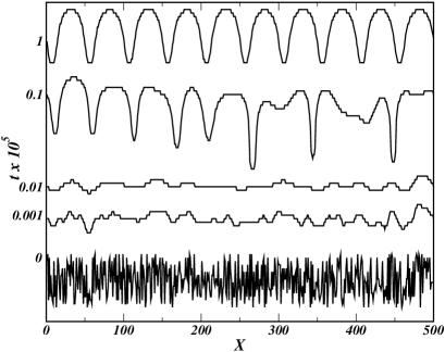
Figure 2: Evolution of cellular pattern from an initial random interface to final state $q_{f}=0.02$ with velocity $v=0.20$ in absence of noise, and $L_{x}=500$.

V Results and Discussion

We perform many simulations of Eq. (4) from various initial conditions in order to verify if a single pattern, out of a number of possible stationary patterns, is indeed selected in the presence of weak noise.

First, simulations are done in the absence of noise $\eta_{\psi}=0=\eta_{c}$ but with initial values of $\psi=\epsilon$ in such a way to form an initial random interface from a uniformly distributed random variable and $c=0$ for convenience. For system widths $L_{x}=250$, $500$ and $1000$ the system always eventually reaches a periodic stationary state with $q_{f}=n/L_{x}=0.020$, where $n$ is the number of cells. For $L_{x}=420$, the final periodicity is $q_{f}=8/420\approx 0.01905$. These results imply that the selected wavevector is the nearest allowed $q_{f}$ to the preferred value for $L_{x}\rightarrow\infty$. In Fig. (2) we show the time evolution of the random interface for $L_{x}=500$, after $t=10^{5}$ time steps the system reaches a pattern with 10 cells, i.e, $q_{f}=0.02$.

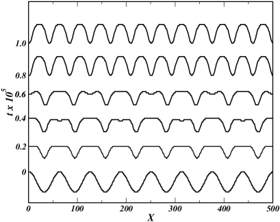
Figure 3: Evolution of cellular pattern of initial periodicity $q_{0}=0.016$ to final state $q_{f}=0.024$ with velocity $v=0.20$ in absence of noise, and $L_{x}=500$.

Second, we run simulations with an initial periodic interface of the form $\zeta(x)=\zeta_{0}{\rm cos}(2\pi q_{0}x)$ with various wavevectors $q_{0}=n_{0}/L_{x}$ and amplitude $\zeta_{0}$ similar to that of the final state of the previous simulation, again in the absence of noise. The initial interface is located at the center of the simulation box of size $L_{x}\times L_{z}$. Simulations with various allowed values of $q_{0}$ and $L_{x}=500$ yield final stationary periodic states with $q_{f}=0.020,0.022\,\,\,{\rm and}\,\,\,0.024$ which determine the Eckhaus stable band of wavevectors for our parameter values. In an infinite system, the Eckhaus band has a continuum of $q$ values which is reduced to a small finite number by the finite width $L_{x}=500$. When the size is doubled to $L_{x}=1000$, we find $7$ wavevectors in the Eckhaus stable band from $q_{x}=0.019\,\,\,{\rm to}\,\,\,0.025$ as expected.

The next simulations study the effect of noise on the evolution of an initial periodic state with wavevector $q_{0}=0.016$ outside the Eckhaus stable band. Without noise, the evolution is by tip splitting of alternate cells to a final wavevector of $q_{f}=0.024$, as shown in Fig. (3). This configuration of $12$ cells is different from the expected wavelength of $q_{f}=0.020$ as obtained from random initial conditions. With applied noise $\eta_{\psi}({\bf r},t)$ independently uniformly distributed with $-\eta<\eta_{\psi}({\bf r},t)<+\eta$ with maximum noise amplitude $\eta=0.10$, the evolution is by a totally different route to the expected state with $q_{S}=0.020$ as shown in Fig. (4). This indicates that noise is essential in the selection of the final state and that only one wavenumber in the Eckhaus band is truly stable in the presence of stochastic noise. We have also performed many simulations, not shown here because of space limitations, with several different initial configurations all of which eventually go to the same state with $q_{f}=0.020$ with only a single exception discussed below.

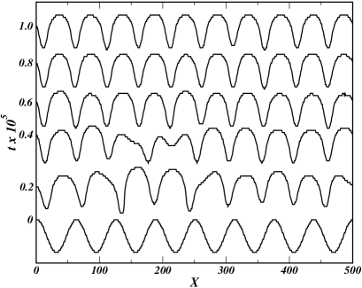
Figure 4: Time evolution of same initial pattern as Fig. (1) with stochastic noise of strength $\eta=0.10$ to final state $q_{f}=0.020$.

Now that we have very strong evidence for selection of a unique wavelength from almost all initial patterns except for some $q_{0}$ in the Eckhaus band, we perform a simulation with an initial pattern $\zeta(x)=\zeta_{0}{\rm cos}(2\pi q_{0}x)$ with $q_{0}=0.024$ with noise to study the stability of modes in the Eckhaus stable band CrossHohenberg ; eckhaus . In the absence of noise, all modes with $q_{0}$ in this band are stable. We impose an interface $\zeta(x)$, evolve it in absence of noise for $10^{4}$ time steps to allow higher harmonics to develop and then evolve the system with noise of strength $\eta=0.20$ for $2\times 10^{5}$ time steps with results shown in Fig. (6). The interface evolves by the gradual loss of one cell to a final configuration of $11$ cells or $q_{f}=0.022$ which remains stable for at least $5\times 10^{7}$ steps. When a brief burst of very strong noise with $\eta>0.25$ is applied and the system then allowed to evolve under weak noise, the expected $q_{S}=0.020$ state results. This is similar to the history dependent effects observed trivedi and discussed theoretically in the absence of noise warrenlanger .

In order to verify our conjecture, we calculate the action from Eq. (14) of the three possible states in the Eckhaus band. As shown in Fig.(5), the action difference $\Delta{\cal S}(\psi,c)\propto\eta^{2}$ so that, for the deterministic case, $\Delta{\cal S}=0$. A finite $\Delta{\cal S}$ is due to finite noise implying that the selection of a particular pattern is due to noise driven fluctuations. Our $L_{x}=500$ system has only three quasi-stationary periodic states in the Eckhaus stable band eckhaus with $q_{x}=0.020,0.022,0.024$ corresponding to $n=10,11,12$ cells. The $q_{S}=0.020$ minimum action state is conjectured to be the unique selected state. An outstanding question is whether pattern selection also holds in the thermodynamic limit $L_{x}=\infty$ when the set of stationary states in the Eckhaus stable band is continuous. Comparing with experiment requires extending the calculation to 3D to study the selected stationary structures of the 2D interface grossmann93 ; plapp04 .

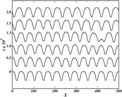
Figure 5: Evolution of an interface with $q_{0}=0.024$ with noise of strength $\eta=0.10$ to a final state $q_{f}=0.022$.

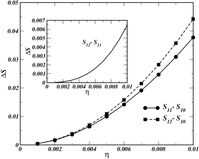
Figure 6: Action differences $\Delta{\cal S}=4\Gamma^{\prime}({\cal S}_{11}-{\cal S}_{10})/{\cal T}$ and $4\Gamma^{\prime}({\cal S}_{12}-{\cal S}_{10})/{\cal T}$ from Eq. (14) in a system width $L_{x}=500$ where the integers $n=q_{x}L_{x}$ in ${\cal S}_{n}$. This shows that the pattern with wavelength $q_{S}=0.020$ has minimum action. The noise is uniformly distributed with $-\eta\leq\eta(\bf{r},t)\leq+\eta$.

These numerical simulations are consistent with the hypothesis of a unique selected stationary state with a definite periodicity $q_{S}=0.020$. This is the noise induced stationary state which is reached from all initial states except from the periodic state with $q_{0}=0.022$ in the Eckhaus stable band. This single state is stable with weak noise up to our longest simulation time. If a unique selected state exists, then only one of these should be stable to weak noise but some are stable within our computation time and it is impractical to perform sufficiently long runs to detect an instability toward the hypothetical minimum action selected state with $q_{S}=0.020$. This study finds that all states with this single exception do evolve to the minimum action state and, in addition, provides some insight into the relative stability of states in the Eckhaus band. On balance, there is overwhelming evidence for our hypothesis of a unique selected state $(\psi,c)$ determined by the minimum of the action ${\cal S}(\psi,c)$ of Eq. (14).

One important caveat must be made. In analogy with a finite equilibrium system jljmk90 , we expect all states in our finite system to have finite lifetimes as the stochastic noise causes transitions between them. We expect that true stationary states exist only in the thermodynamic limit of $L\rightarrow\infty$ when the lifetime of the selected state should be infinite but this limit is extremely difficult to approach numerically for well known and obvious reasons. If a finite size scaling theory existed for these dynamical processes, the $L\rightarrow\infty$ limit could be studied by the methods of this letter. However, to the best of our knowledge, such a scaling theory does not exist.

VI Acknowledgements

This work was supported by a NSF-CNPq grant (E.G. and J.M.K.), by CNPq (R.N.C.F.) and FAPESP (No. 03/00541-0) (E.G.).

References

- (1) M.C. Cross and P. C. Hohenberg, Rev. Mod. Phys. 65, 851 (1993)
- (2) J. Bechhoefer and A. Libchaber, Phys. Rev. B 35, 1393 (1987)
- (3) B. Billia, H. Jamgotchian and L. Capella, J. Cryst. Growth 82, 747 (1987)
- (4) J.-M. Flesselles, A. J. Simon and A. J. Libchaber, Adv. Phys. 40, 1 (1991)
- (5) K. A. Jackson and J. D. Hunt, Trans. AIME 236, 1129 (1966)
- (6) M. Ginibre, S. Akamatsu and G. Faivre, Phys. Rev. E 56, 780 (1997)
- (7) A. Karma, Phys. Rev. Lett. 57, 858 (1986)
- (8) M. Kerszberg, Phys. Rev. B 27, 3909 (1983)
- (9) M. Kerszberg, Phys. Rev. B 27, 6796 (1983)
- (10) M. Kerszberg, Phys. Rev. B 28, 247 (1983)
- (11) D. A. Kurtze, Phys. Rev. Lett. 77, 63 (1996)
- (12) T. Dombre and V. Hakim, Phys. Rev. A 36, 2811 (1987)
- (13) M. Ben Amar and B. Moussallam, Phys. Rev. Lett. 60, 317 (1988)
- (14) J. Swift and P. C. Hohenberg, Phys. Rev. A 15, 319 (1977); 46, 4773 (1992).
- (15) E. Hernández-García, J. Viñals, R. Toral, and M. San Miguel, Phys. Rev. Lett.70, 3576 (1993).
- (16) B. Grossmann, K. R. Elder, M. Grant and J. M. Kosterlitz, Phys. Rev. Lett. 71, 3323 (1993)
- (17) K. R. Elder, F. Drolet, J. M. Kosterlitz and M. Grant, Phys. Rev. Lett. 72, 677 (1994)
- (18) F. Drolet, K. R. Elder, M. Grant and J. M. Kosterlitz, Phys. Rev. E 61, 6705 (2000)
- (19) R. Kobayashi, Physica D 63, 410 (1993)
- (20) A. Karma and W.-J. Rappel, Phys. Rev. E 57, 4323 (1998)
- (21) K. R. Elder, M. Grant, N. Provatas and J. M. Kosterlitz, Phys. Rev. E 64, 021604 (2001)
- (22) P. C. Hohenberg and B. I. Halperin, Rev. Mod. Phys. 49, 435 (1977)
- (23) R. Graham and R. Tél, Phys. Rev. A 31, 1109 (1985);42, 4661 (1990).
- (24) R. Montagne, E. Hernández-García, and M. San Miguel, Physica D 96, 47 (1996).
- (25) R. Landauer, Physica A 194, 551 (1993).
- (26) M. I. Dykman, B. Golding, I. L. McCann, V. N. Smelyanskiy, D. G. Luchinsky, R. Mannella, and P. V. E. McClintock, Chaos 11, 587 (2001)
- (27) M. I. Dykman, B. Golding, and D. Ryvkine, Phys. Rev. Lett. 92, 080602 (2004)
- (28) M. Mardar, Phys. Rev. Lett. 74, 4547 (1995)
- (29) L. Bertini, A. De Sole, D. Gabrielli, G. Jona-Lasinio and C. Landim, Phys. Rev. Lett. 87, 040601 (2001)
- (30) C. De Dominicis, and L. Peliti, Phys. Rev. B 18, 353 (1978).
- (31) P. C. Martin, E. D. Siggia, and H. A. Rose, Phys. Rev. A 8, 423 (1973)
- (32) V. Eckhaus, Studies in Nonlinear Stability Theory, Springer Tracts in Natural Philosophy, Vol. 6, (1965) (Springer-Verlag, Berlin)
- (33) R. Trivedi and K. Somboonsuk, Acta Metall. 33, 1061 (1985).
- (34) J. A. Warren and J. S. Langer, Phys. Rev. E 47, 2702 (1993).
- (35) H. C. Fogedby, Phys. Rev. E 59, 5065 (1999)
- (36) A. J. Simon, J. Bechhoefer, and A. Libchaber, Phys. Rev. Lett. 61, 2574 (1988).
- (37) M. Plapp and M. Dejmek, Europhys. Lett. 65, 376 (2004).
- (38) J. Lee and J. M. Kosterlitz, Phys. Rev. Lett. 65, 137 (1990)