Dynamics of trapped bright solitons in the presence of localized inhomogeneities

Abstract

We examine the dynamics of a bright solitary wave in the presence of a repulsive or attractive localized “impurity” in Bose-Einstein condensates (BECs). We study the generation and stability of a pair of steady states in the vicinity of the impurity as the impurity strength is varied. These two new steady states, one stable and one unstable, disappear through a saddle-node bifurcation as the strength of the impurity is decreased. The dynamics of the soliton is also examined in all the cases (including cases where the soliton is offset from one of the relevant fixed points). The numerical results are corroborated by theoretical calculations which are in very good agreement with the numerical findings.

1 Introduction

In the past few years, the rapid experimental and theoretical developments in the field of Bose-Einstein condensates (BECs) reviews have led to a surge of interest in the study of the nonlinear matter waves that appear in this context. More specifically, experiments have yielded bright solitons in self-attractive condensates (⁷Li) in a nearly one-dimensional setting expb , as well as their dark expd and, more recently, gap Oberthaler counterparts in repulsive condensates, such as ⁸⁷Rb. The study of these matter-wave solitons, apart from being a topic of interest in its own right, may also have important applications. For instance, a soliton may be transferred and manipulated similarly to what has been recently shown, experimentally and theoretically, for BECs in magnetic waveguides aw and atom chips ac . Furthermore, similarities between matter and light waves suggest that some of the technology developed for optical solitons ka may be adjusted for manipulations with MWs, and thus applied to the rapidly evolving field of quantum atom optics (see, e.g., mo ).

One of the topics of interest in this context is how matter-waves can be steered/manipulated by means of external potentials, currently available experimentally. In addition to the commonly known magnetic trapping of the atoms in a parabolic potential, it is also experimentally feasible to have a sharply focused laser beam, such as ones already used to engineer desired density distributions of BECs in experiments expd . Depending on whether it is blue-detuned or red-detuned, this beam repels or attracts atoms, thus generating a localized “defect” that can induce various types of the interaction with solitary matter waves. This possibility was developed to some extent in theoretical theor and experimental exper studies of dynamical effects produced by moving defects, such as the generation of gray solitons and sound waves in one dimension rad2325 , and formation of vortices in two dimensions (see, e.g., mplb and references therein). The interaction of dark solitons with a localized impurity was also studied dimitri .

Our aim here is to examine the interaction of a bright matter-wave soliton with a strongly localized (in fact, $\delta$-like) defect, in the presence of the magnetic trap. Our approach is different from that of Ref. dimitri , in that we will view the presence of the defect as a bifurcation problem. We demonstrate that the localized perturbation (independently of whether it is attractive or repulsive) creates an effective potential that results in two additional localized states (one of which is naturally stable, while the other is always unstable) for sufficiently large impurity strength. As one may expect on grounds of the general bifurcation theory, these states will disappear, “annihilating” with each other, as the strength of the impurity is decreased below a threshold value. We will describe this saddle-node bifurcation in the present context. We will also compare our numerical predictions for its occurrence with analytical results following from an approximation that treats the soliton as a quasi-particle moving an effective potential. Very good agreement between the analytical and numerical results will be demonstrated. Finally, we will examine the dynamics of solitons inside the combined potential, jointly created by the magnetic trap and the localized defect. Both equilibrium positions and motion of the free soliton will be considered in the latter case.

The paper is structured as follows: in Section 2, we present our effective potential theory. In Section 3, we discuss numerical methods and results, and provide their comparison with the analytical predictions. Finally, in Section 4, we summarize our findings and present our conclusions.

2 Setup and Theoretical Results

In the mean-field approximation, the single-atom wavefunction for a dilute gas of ultra-cold atoms very accurately obeys the Gross-Pitaevskii equation (GPE). Although the GPE naturally arises in the three-dimensional (3D) settings, it has been shown theory ; Isaac ; Salasnich that it can be reduced to its one-dimensional (1D) counterpart for the so-called cigar-shaped condensates. Cigar-shaped condensates are created when two transverse directions of the atomic cloud are tightly confined, and the condensate is effectively rendered one-dimensional, by suppressing dynamics in the transverse directions. The effective equation describing this quasi-1D is simply tantamount to a directly written 1D GPE. In normalized units, it takes the well-known from,

$$iu_{t}=-\frac{1}{2}u_{xx}+g|u|^{2}u+V(x)u,$$ (1)

where subscripts denote partial derivatives and $u(x,t)$ is the one-dimensional mean-field wave function. The normalized 1D atomic density is given by $n=|u(x,t)|^{2}$, while the total number of atoms is proportional to the norm of the normalized wavefunction $u(x,t)$, which is an integral of motion of Eq. (1):

$$P=\int_{-\infty}^{+\infty}|u(x,t)|^{2}dx.$$ (2)

The nonlinear coefficient in Eq. (1) is $g=\pm 1$, for repulsive or attractive interatomic interactions respectively. Finally, the magnetic trap, together with the localized defect, are described by a combined potential $V(x)$ of the form

$$V(x)=\frac{1}{2}\Omega^{2}x^{2}-V_{0}\delta(x-\xi).$$ (3)

In Eqs. (1) and (3), the space variable $x$ is given in units of the healing length $\tilde{\xi}=\hbar/\sqrt{n_{0}g_{1D}m}$, where $n_{0}$ is the peak density, and the normalized atomic density is measured in units of $n_{0}$. Here, the nonlinear coefficient is considered to have an effectively 1D form, namely $g_{1D}\equiv g_{3D}/(2\pi l_{\perp}^{2})$, where $g_{3D}=4\pi\hbar^{2}a/m$ is the original 3D interaction strength ($a$ is the scattering length, $m$ is the atomic mass, and $l_{\perp}=\sqrt{\hbar/m\omega_{\perp}}$ is the transverse harmonic-oscillator length, with $\omega_{\perp}$ being the transverse-confinement frequency). Further, time $t$ is given in units of $\tilde{\xi}/c$ (where $c=\sqrt{n_{0}g_{1D}/m}$ is the Bogoliubov speed of sound), and the energy is measured in units of the chemical potential, $\mu=g_{1D}n_{0}$. Accordingly, the dimensionless parameter $\Omega\equiv\hbar\omega_{x}/g_{1D}n_{0}$ (where $\omega_{x}$ is the confining frequency in the axial direction) determines the effective strength of the magnetic trap in the 1D rescaled equations. Positive and negative values of $V_{0}$ corresponds, respectively, to the attractive and repulsive defect. Finally, since we are interested in bright matter-wave solitons, which exist in the case of attraction, we hereafter set the normalized nonlinear coefficient $g=-1$.

It is worth mentioning that modified versions of the 1D GPE are known too. One of them features a non-polynomial nonlinearity, instead of the cubic one in Eq. (1) Salasnich . A different equation was derived for a case of a very strong nonlinearity, so that the local value of the potential energy exceeds the transverse kinetic energy. It amounts to the same cubic equation (1), but with a noncanonical normalization condition, with the integral in Eq. (2) replaced by $\int_{-\infty}^{+\infty}\left|u(x,t)\right|^{4}dx$.

In the absence of potential, Eq. (1) supports stationary soliton solutions of the form

$$u_{s}(x)=\eta\,\mathrm{sech}\left[\eta(x-\zeta)\right]\exp\left(i\eta^{2}t/2\right)$$ (4)

where $\eta$ is an arbitrary amplitude and $\zeta$ is the position of the soliton’s center. It is possible to generate moving solitons (with constant velocity) by application of the Galilean boost to the stationary soliton in Eq. (4).

One can examine the persistence and dynamics of the bright solitary waves in the presence of the potential $V(x)$ by means of the standard perturbation theory (see e.g., Ref. RMP ; sb and a more rigorous approach, based on the Lyapunov-Schmidt reduction, that was developed in Ref. kapitula ). This method, which treats the soliton as a particle, yields effective potential forces acting on the particle from the defect and the magnetic trap,

$$F_{\mathrm{def}}=2\eta^{3}\tanh(\eta(\xi-\zeta))\,\mathrm{sech}^{2}(\eta(\xi-\zeta))V_{0},$$ (5)

$$F_{\mathrm{trap}}=-2\Omega^{2}\zeta\eta,$$ (6)

which enter the equation of motion for $\zeta(t)$:

$$\ddot{\zeta}=F_{\mathrm{imp}}+F_{\mathrm{trap}}.$$ (7)

Below, results following from this equation will be compared to direct simulations of Eq. (1).

The stationary version of Eq. (7) ($\ddot{\zeta}=0$),

$$\left(\eta^{3}V_{0}/\Omega^{2}\right)\left(\tanh\theta\right)\mathrm{sech}^{2}\theta=\eta\xi-\theta,$$ (8)

with $\theta\equiv\eta(\xi-\zeta)$, determines equilibrium positions ($\zeta$) of the soliton’s center. Depending on parameters, this equation may have one or three physical solutions, see below. In what follows, we will examine the solutions in detail and compare them to numerical results stemming from direct simulations of Eq. (1).

3 Numerical Methods and Results

In order to numerically identify standing wave solutions of Eq. (1), we substitute, as usual, $u(x,t)=\exp(i\Lambda t)w(x)$, which results in the steady-state problem:

$$\Lambda w=\frac{1}{2}w_{xx}+w^{3}-V(x)w.$$ (9)

This equation is solved by a fixed-point iterative scheme on a fine finite-difference grid. Then, we analyze the stability of the obtained solutions by using the following ansatz for the perturbation,

$$u(x)=e^{i\Lambda t}\left[w(x)+a(x)e^{-\lambda t}+b^{\ast}(x)e^{-\lambda^{\star}t}\right]$$ (10)

(the asterisk stands for the complex conjugation), and solving the resulting linearized equations for the perturbation eigenmodes $\{a(x),b(x)\}$ and eigenvalues $\lambda$ associated with them. The resulting solutions are also used to construct initial conditions for direct numerical simulations of Eq. (1), to examine typical scenarios of the full dynamical evolution. To eliminate effects of the radiation backscattering in these simulations, we have used absorbing boundary layers, by adding a term in Eq. (1), of the form:

$$\begin{array}[]{rcl}\Gamma u&=&-\,\left[(1+\tanh(1000(x-R))\right.\\[8.61108pt] &&\left.+\,\,\,(1-\tanh(1000(x-L))\right]\,u,\end{array}$$ (11)

which is defined on the domain $L<x<R$. In the numerical simulations presented herein, the $\delta$-function of the potential was approximated by a Gaussian waveform, according to the well-known formula,

$$\delta(x)=\lim_{\sigma\rightarrow 0^{+}}\frac{1}{\sqrt{2\pi}\sigma}\exp\left(-\frac{x^{2}}{4\sigma}\right).$$ (12)

Lorentzian and hyperbolic-function approximations to the $\delta$-function were also used, without producing any conspicuous difference in the results.

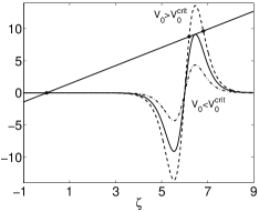
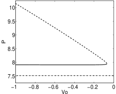
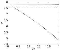
Figure 1: Saddle-node bifurcation of stationary states for the location $\zeta$ of the bright soliton inside the magnetic trap ($\Omega=0.1$), with the localized defect of strength $V_{0}$ located at $\xi=6$. The top-left panel displays the corresponding solutions of the stationary equation (8). For the weak defect, dash-dotted line, only one steady state exists very close to the origin. As the defect’s strength increases, two additional fixed points (both located on the same side of the impurity) are created in a saddle-node bifurcation. The top-right panel depicts the position and stability (solid for stable and dashed for unstable) for the steady states as a function of the defect’s strength $V_{0}$. The thin horizontal line for $\xi=6$ shows the location of the defect. The two bottom plots depict another version of the stability diagram, in terms of the soliton’s norm $P$ [see Eq. (2)], as $V_{0}$ is varied.

As mentioned above, depending on the value of the defect’s strength $V_{0}$, Eq. (8) may have either one or three physical roots for $\zeta$ (the equilibrium position of the soliton’s center). The border between these two generic cases is a separatrix where two of the roots merge in one before they disappear. All the qualitatively different cases are depicted in the top-left panel of Fig. 1. The physical interpretation of this result can be given as follows. Obviously, in the absence of the defect there exists a stable solitary-wave configuration centered at $\zeta=0$ (hence there is a single steady state in the problem). On the other hand, it is easy to see that Eq. (8) generates three solutions for large $V_{0}$. Hence, there should be a bifurcation point, of the saddle-node type, that leads to the disappearance of two branches of the solutions as $V_{0}$ decreases. Furthermore, based on general bifurcation theory principles, one of the steady states disappearing as a result of the bifurcation may correspond to a stable soliton, whereas its companion branch definitely represents an unstable solitary wave. The full bifurcation-diagram scenario, for the position of the soliton’s center and its norm, is depicted in Fig. 1. It is interesting to note that the norm of the solitons corresponding to the unstable branches varies almost linearly with the defect’s strength, while the stable branches correspond to solitons whose norm is approximately constant.

The qualitative predictions about the nature of the steady states and their stability have been tested for repulsive and attractive defects, as shown in Figs. 2 and 3, respectively. In these figures, three left panels show the spatial profiles of the stable branch at $\zeta=0$, and the unstable and stable branches in the neighborhood of the defect. The middle panels show the temporal evolution of each one of these solutions, while the right panels show the results of the linear stability analysis. The latter set clearly illustrates the instability of the middle branch due to the presence of a real eigenvalue pair. It is also noteworthy that, in the case of the repulsive defect (in which case an unstable solution is centered at the defect) the soliton oscillates around the nearby stable steady state, shedding radiation waves, cf. Fig. 2. On the other hand, in the attractive case the unstable solution centered beside the defect is “captured” by the defect, resulting in its trapping at the defect’s center, cf. Fig. 3. However, a fraction of the condensate is also emitted from the defect in the process, leading to oscillations that can be observed in the respective space-time-evolution panel.

To verify the analytical results following from Eqs. (7) and (8), we have compared the analytically predicted critical value of $V_{0}$ (for which a double root appears) with the numerically obtained turning point for the saddle-node bifurcation. This comparison was performed for many values of the impurity center $\xi$. In fact, the critical value was predicted using two different forms of the analytical prediction: one with the Dirac $\delta$-function proper, and another one with the Gaussian approximation for the $\delta$-function and an accordingly modified version of Eq. (8), namely

$$F_{\mathrm{imp}}+F_{\mathrm{trap}}=\int\limits_{-\infty}^{\infty}V(x)\frac{\partial}{\partial x}\left(\left|u(x)\right|^{2}\right)dx=0,$$ (13)

with the function $V(x)$ incorporating the parabolic magnetic trap and the Gaussian impurity terms. Here the integration was performed with the numerically implemented $V(x)$, and the best fit of $u(x)$ to a hyperbolic secant waveform has been used in Eq. (13). The parameter values along with the resulting critical values of $V_{0}$ are given in Fig. 4. In all cases, the numerical results for the bifurcation point closely match the theoretical predictions.

Having examined statics and dynamics in the vicinity of the stable and unstable fixed points of the system, we now turn to an investigation of the dynamics, setting the initial soliton farther away from the equilibrium positions. Figure 5 displays three typical examples, with the soliton set to the left and to the right of the repulsive (and of the attractive) defect. In the repulsive case, we observe that the soliton is primarily reflected from the defect; however, when it has large kinetic energy at impact (which takes place if it was initially put at a position with large potential energy), a fraction of the matter is transmitted through the defect. On the other hand, in the attractive case, a fraction of the matter is always trapped by the defect. However, this fraction is smaller when the kinetic energy at impact is larger.

We note in passing that, while Eq. (7) can predict not only the equilibrium positions of the soliton but also the dynamical behavior of $\zeta(t)$, we have opted not to use it for the numerical experiments. The main reason is that, as can be clearly inferred from Figs. 2-3 and 5, the interaction of the solitary wave with the defect entails emission of a sizable fraction of matter in the form of small-amplitude waves, which, in turn, may interfere with the solitary wave and significantly alter his motion (see e.g., Fig. 5). Hence, the prediction of the dynamics based on the adiabatic approximation, which is implied in Eq. (7), would be inadequate in the presence of these phenomena.

4 Conclusions

In this work, we have examined the interaction of bright solitary waves with localized defects in the presence of magnetic trapping, which is relevant to Bose-Einstein condensates with negative scattering lengths. We have found that the defect induces, if its strength is sufficiently large, the existence of two additional steady states (bifurcating into existence through a saddle-node bifurcation), one of which is stable and one unstable. We have constructed the relevant bifurcation diagram and explicitly found both the stable and the unstable solutions, and quantified the instability of the latter via the presence of a real eigenvalue pair. The dynamical instability of these unstable states leads to oscillations around (for repulsive defects) and/or trapping at (for attractive defects) the nearby stable steady state. Additionally, we have developed a collective-coordinate approximation to explain the steady soliton solutions and the corresponding bifurcation. We have illustrated the numerical accuracy of the analytical approximation by comparison with direct numerical results. We have also displayed, through direct numerical simulations, the dynamics which follows setting the initial soliton off a steady-state location. Noteworthy phenomena that occur in this case are the emission of radiation by the soliton colliding with the repulsive defect, and capture of a part of the matter by the attractive one.

These results may be relevant to the trapping, manipulation and guidance of solitary waves in the context of BEC. They illustrate the potential of the combined effect of magnetic and optical (provided by a focused laser beam) trapping to capture (either at or near the laser-beam-induced local defect) a solitary wave which can be subsequently guided, essentially at will. Naturally, the beam’s intensity must exceed a critical value, which can be explicitly calculated in the framework of the developed theory. It would be particularly interesting to examine the predicted soliton dynamics in BEC experiments.

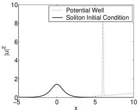
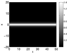
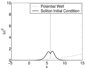
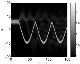
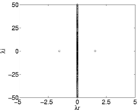
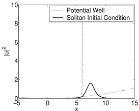
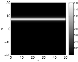
Figure 2: Steady states of the bright soliton for the repulsive defect: $V_{0}=-1$, $\sigma=0.045$, $\eta=\sqrt{2}$, $\Omega=0.1$ and $\xi=6$. The first row corresponds to the steady state at $\zeta=0$, the second row to the steady state centered at the defect, and the third row to the steady state trapped to the right of the impurity. For each row, the left panel displays the numerically exact steady-state soliton profile, the middle panel is the space-time evolution shown by means of contour plots, and the right graph shows the spectral plane ($\lambda_{r},\lambda_{i}$) for the stability eigenvalues $\lambda=\lambda_{r}+i\lambda_{i}$ corresponding to this solution. For the two stable steady states (trapped at the defect and to the right of it), the solution remains stationary as expected. On the other hand, for the unstable steady state, after approximately 20 time units, the instability fragments the soliton into a more localized part oscillating to its right and a more extended part oscillating to its left.

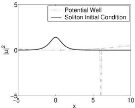
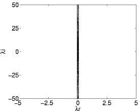
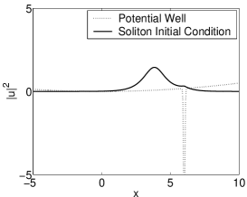
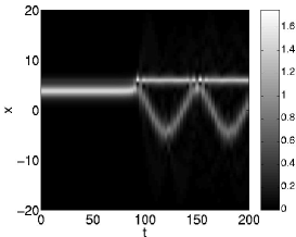
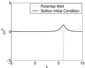
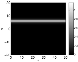
Figure 3: Same as in the previous figure, but for an attractive defect: $V_{0}=-1$, $\sigma=0.045$, $\eta=\sqrt{2}$, $\Omega=0.1$ and $\xi=6$. Notice that now the unstable steady state is to the left of the attractive defect, while its unstable time-evolution leads to its trapping at the defect.

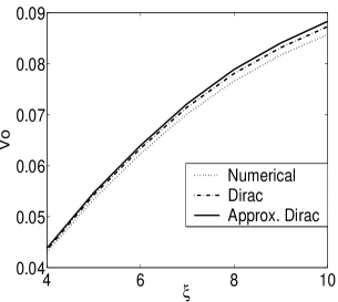
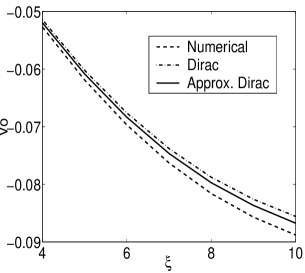
Figure 4: Critical values of $V_{0}$, corresponding to the disappearance of two steady states, for $\sigma=0.045$. The left and right graphs pertain to the attractive and repulsive defect, respectively.

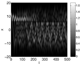
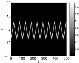
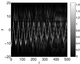
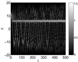
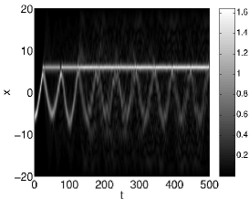
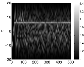
Figure 5: Examples of the soliton interaction with the repulsive defect (top panels) and the attractive one (bottom panels) located at $\xi=6$. The soliton is initially offset with respect to the steady states of the model. For all cases, the parameters are $V_{0}=\pm 1$, $\sigma=0.045$ and $\eta=\sqrt{2}$. The initial position of the soliton is $\zeta_{0}=12,-6,-12$, for the plots from left to right. In the repulsive case (top panels), the soliton is primarily reflected by the defect (with a small transmitted fraction of the norm). Similar behavior was observed for other values of $\zeta$, with the amount of material passing through the defect increasing with $\zeta_{0}$. On the other hand, in the attractive case (bottom panels), the soliton gets fragmented into reflected, trapped and transmitted parts. For larger initial values of $\zeta$, the trapped fraction is smaller.

References

- (1) F. Dalfovo, S. Giorgini, L. P. Pitaevskii, and S. Stringari, Rev. Mod. Phys. 71, 463 (1999); A. J. Leggett, ibid. 73, 307 (2001); E. A. Cornell and C. E. Wieman, ibid. 74, 875 (2002); W. Ketterle, ibid. 74, 1131 (2002).
- (2) K. E. Strecker, G. B. Partridge, A. G. Truscott, and R. G. Hulet, Nature 417, 150 (2002); L. Khaykovich, F. Schreck, G. Ferrari, T. Bourdel, J. Cubizolles, L. D. Carr, Y. Castin, and C. Salomon, Science 296, 1290 (2002);
- (3) S. Burger, K. Bongs, S. Dettmer, W. Ertmer, K. Sengstock, A. Sanpera, G. V. Shlyapnikov, and M. Lewenstein, Phys. Rev. Lett. 83, 5198 (1999); J. Denschlag, J. E. Simsarian, D. L. Feder, C. W. Clark, L. A. Collins, J. Cubizolles, L. Deng, E. W. Hagley, K. Helmerson, W. P. Reinhardt, S. L. Rolston, B. I. Schneider, and W. D. Phillips, Science 287, 97 (2000); B.P. Anderson, P. C. Haljan, C. A. Regal, D.L. Feder, L. A. Collins, C. W. Clark, and E. A. Cornell, Phys. Rev. Lett. 86, 2926 (2001).
- (4) B. Eiermann, Th. Anker, M. Albiez, M. Taglieber, P. Treutlein, K.-P. Marzlin, and M. K. Oberthaler, Phys. Rev. Lett. 92, 230401 (2004).
- (5) A. E. Leanhardt, A. P. Chikkatur, D. Kielpinski, Y. Shin, T. L. Gustavson, W. Ketterle, and D. E. Pritchard, Phys. Rev. Lett. 89, 040401 (2002); H. Ott, J. Fortagh, S. Kraft, A. Gunther, D. Komma, and C. Zimmermann, Phys. Rev. Lett. 91, 040402 (2003);
- (6) W. Hänsel, P. Hommelhoff, T. W. Hansch, and J. Reichel, Nature 413, 498 (2001); R. Folman and J. Schmiedmayer, Nature 413, 466 (2001); J. Reichel, Appl. Phys. B 74, 469 (2002); R. Folman, P. Krueger, J. Schmiedmayer, J. Denschlag and C. Henkel, Adv. Atom. Mol. Opt. Phys. 48, 263 (2002).
- (7) Yu. S. Kivshar and G. P. Agrawal, Optical Solitons: From Fibers to Photonic Crystals (Academic Press, San Diego, 2003).
- (8) K. Mølmer, New J. Phys. 5, 55 (2003).
- (9) T. Frisch, Y. Pomeau and S. Rica, Phys. Rev. Lett. 69, 1644 (1992); T. Winiecki, J. F. McCann and C. S. Adams, Phys. Rev. Lett. 82, 5186 (1999); B. Jackson, J. F. McCann and C. S. Adams, Phys. Rev. A 61, 013604 (2000); G. E. Astracharchik, L.P. Pitaevskii, Phys. Rev. A 70, 013608 (2004).
- (10) C. Raman, M. Köhl, D. S. Durfee, C. E. Kuklewicz, Z. Hadzibabic and W. Ketterle, Phys. Rev. Lett. 83, 2502 (1999); R. Onofrio, C. Raman, J.M. Vogels, J. R. Abo-Shaeer, A.P. Chikkatur and W. Ketterle, Phys. Rev. Lett. 85, 2228 (2000).
- (11) V. Hakim, Phys. Rev. E 55, 2835 (1997); P. Leboeuf and N. Pavloff, Phys. Rev. A 64, 033602 (2001); N. Pavloff, Phys. Rev. A 66, 013610 (2002); A. Radouani, Phys. Rev. A, 70, 013602 (2004); G. Theocharis, P.G. Kevrekidis, H.E. Nistazakis, D.J. Frantzeskakis and A.R. Bishop, Phys. Lett. A, in press.
- (12) P. G. Kevrekidis, R. Carretero-González, D.J. Frantzeskakis, and I.G. Kevrekidis, Mod. Phys. Lett. B 18, 1481 (2004).
- (13) D. J. Frantzeskakis, G. Theocharis, F. K. Diakonos, P. Smelcher and Yu.S. Kivshar, Phys. Rev. A 66, 053608 (2002).
- (14) V. M. Pérez-García, H. Michinel and H. Herrero, Phys. Rev. A 57, 3837 (1998); for a more rigorous derivation of the 1D effective equation (in the case of repulsion, rather than attraction), see a paper by E.H. Lieb, R. Seiringer, and J. Yngvason, Phys. Rev. Lett. 91, 150401 (2003).
- (15) Y. B. Band, I. Towers, and B. A. Malomed, Phys. Rev. A 67, 023602 (2003).
- (16) L. Salasnich, A. Parola and L. Reatto, Phys. Rev. A 65, 043614 (2002).
- (17) Yu. S. Kivshar and B. A. Malomed, Rev. Mod. Phys. 61, 763 (1989).
- (18) R. Scharf and A. R. Bishop, Phys. Rev. E 47, 1375 (1993).
- (19) T. Kapitula, Physica D 156, 186 (2001).