The Gross-Pitaevskii Equation for Bose Particles in a Double Well Potential: Two Mode Models and Beyond

Abstract

There have been many discussions of two-mode models for Bose condensates in a double well potential, but few cases in which parameters for these models have been calculated for realistic situations. Recent experiments lead us to use the Gross-Pitaevskii equation to obtain optimum two-mode parameters. We find that by using the lowest symmetric and antisymmetric wavefunctions, it is possible to derive equations for a more exact two-mode model that provides for a variable tunneling rate depending on the instantaneous values of the number of atoms and phase differences. Especially for larger values of the nonlinear interaction term and larger barrier heights, results from this model produce better agreement with numerical solutions of the time-dependent Gross-Pitaevskii equation in 1D and 3D, as compared with previous models with constant tunneling, and better agreement with experimental results for the tunneling oscillation frequency [Albiez et al., cond-mat/0411757]. We also show how this approach can be used to obtain modified equations for a second quantized version of the Bose double well problem.

I Introduction

The analogy between double Bose condensates, separated by a barrier, and Josephson oscillations of superconductors Josephson was apparently first suggested by Javanainen Juha1 , and has been developed more thoroughly in a number of theoretical studies Walls ; Milburn ; Smerzi ; Zapata ; Steel ; Spekkens ; Ivanov ; Raghavan ; Kivshar ; Fran ; Paraoanu ; Leggett ; Anglin ; Mahmud1 ; Mahmud2 ; Links . Especially from work in Milburn ; Smerzi ; Raghavan and more recently in Fran ; Mahmud2 , a rather elaborate picture of phase space dynamics has now been developed. The equations for tunneling oscillations of Bose condensates in a double well potential have been shown to resemble a pendulum whose length depends on the momentum. In the limit of small amplitude oscillations, the equations are the same as for Josephson oscillations for superconductors separated by a weak link Averin . It has also been shown that when atom-atom interactions exceed a critical value, the ensemble will remain trapped in one well while the phase continually increases, resembling a pendulum with sufficient energy to rotate.

Experiments showing interference when condensates in a potential with a barrier were released Andrews first stimulated interest in the problem of Bose condensates in a double well potential. More pertinent to the present discussion are experiments that probe the evolution of the distribution between two or more wells of an optical lattice. Josephson oscillations have been observed in 1D optical potential arrays Inguscio . Recently for a double well potential, both the regimes of tunneling and self-trapping of Rb atoms were observed Albiez . In view of proposed extensions of these and other experimental techniques, Peil ; Zimmerman ; Williams ; Hu ; Reichel , it seems appropriate now to reexamine the theory with the goal of developing models to deal with more diverse conditions.

It is often assumed that the “tight-binding” approximation is valid, leading to what is known as the Bose-Hubbard model Fisher ; Jaksch , or discrete nonlinear Schrödinger equation Trombettoni ; Rey . This model, which has been confirmed under the experimental conditions of Inguscio , employs parameters for tunneling and on-site energy that are usually taken to be constant. One expects that with sufficiently large numbers of atoms, the atom-atom repulsion will cause the wavefunctions in a well to vary in size depending on the atom number, and consequently, the tunneling parameter and onsite energy might vary.

We have found that it is possible to solve a more exact two-mode model based on symmetric and antisymmetric solutions of the Gross-Pitaevskii equation Kivshar ; BAPS . For weak interactions, this new two-mode model produces negligible differences from previous two-mode models. However, for larger interactions, there are substantial differences and it turns out that the recent experiments Albiez begin to sample the regime in which the differences are significant. In this report, we show that the new two-mode model implies a tunneling parameter that can vary with time, depending on the number and phase of the ensemble in each well, hence the name “variable tunneling model” (VTM). Despite the additional terms needed to produce this result, the equations eventually reduce to equations with the same form as the usual Bose-Josephson junction equations, but with parameters defined differently, and with one new term that can be significant in the case of strong interactions. Below, we compare results obtained with this model to those with a two-mode model with constant tunneling, with results of a multi-mode model, and then with numerical solutions of the time-dependent Gross-Pitaevskii equation (TDGPE). The parameters used in the two- or multi-mode models are obtained from numerical solution of the stationary Gross-Pitaevskii (GP) equation, so it is perhaps not surprising that the model that mimics the GP equation most closely also best reproduces results from the TDGPE. For very large interactions, results from any two-mode model will deviate from the TDGPE results, but agreement is most persistent with the VTM. Under conditions of a particular experiment, effects of non-zero temperature and experimental uncertainties may be larger than the differences shown below.

The present study is primarily limited to a mean-field approach using the GP equation, assuming that fluctuations and thermal excitations are negligible and without quantizing particle number. Because atom number is not quantized, the particle number difference and phase difference of atoms in two wells or two modes are classical quantities in this approach. Considerable theoretical effort has been devoted to the second quantized form Milburn ; Steel ; Spekkens ; Ivanov ; Links ; Mahmud2 . We show below that our approach can be used to obtain more exact equations for quantization, and we apply these equations to the case of weakly interacting systems to show the connection between first and second quantized theories in this limited regime. As shown in Mahmud2 , the classical patterns appear clearly in the quantum phase space picture with as few as 10 atoms. For experiments that involve on the order of 1,000 atoms, it seems useful to have an improved GP (mean-field) approach.

An outline of this paper is as follows. Section II is devoted to 1D models. We first (Section IIA) derive the new (VTM) two-mode equations, and then (Section IIB) compare with previous approaches. Section IIC lays out a multi-mode approach, Section IID discusses dynamics in phase space, Section IIE gives equations for a second-quantized version. Experiments are of course in 3D, with some degree of transverse confinement. Therefore in Section III we present a formalism for 3D calculations and give a few results, including comparisons with the experimental results of Albiez .

II Models

II.1 Time-Dependent Gross-Pitaevskii Equation

When the temperature is sufficiently low and when particle numbers are sufficient that second quantization effects are not important, the time-dependent Gross-Pitaevskii Equation (TDGPE) may be used for the wave function $\psi(x,t)$ for interacting Bose condensate atoms at zero temperature in an external potential $V_{ext}(x)$. Letting $\hbar=m=1$, a dimensionless version is

$$i\frac{\partial\psi}{\partial t}=-\frac{1}{2}\frac{\partial^{2}\psi}{\partial x^{2}}+V_{\rm{ext}}\psi+g|\psi|^{2}\psi.$$ (1)

The relationship between $g$ and $g_{3D}$ will be discussed in section IIIA. Here $\int dx|\psi(x,t)|^{2}=N$, where $N$ is the number of atoms. Except in Sec. II.6, $N$ is not quantized, and the approach is strictly mean-field.

We consider double-well potentials $V_{ext}(x)$ that are symmetric in $x$. Initially, we discuss one-dimensional versions. Under the above conditions, we will use results obtained with the TDGPE to test two-mode and multimode models discussed below. The TDGPE can tell us, for example, whether the phase is nearly constant as a function of $x$ over an individual well.

II.2 New Two Mode Model

In many situations, a good approximation is obtained with a two mode representation of $\psi(x,t)$. In early work Milburn , wavefunctions localized in each well were used. Later, $\pm$ combinations of symmetric and antisymmetric functions, as in Smerzi ; Raghavan ; Kivshar provided a more accurate formulation, and we follow the approach of Kivshar here:

$$\psi(x,t) = \sqrt{N}[\psi_{1}(t)\Phi_{1}(x)+\psi_{2}(t)\Phi_{2}(x)];$$ (2)

$$\Phi_{1,2}(x) = \frac{\Phi_{+}(x)\pm\Phi_{-}(x)}{\sqrt{2}},$$ (3)

where

$$\Phi_{\pm}(x)=\pm\Phi_{\pm}(-x);\ \ \int dx\Phi_{i}\Phi_{j}=\delta_{i,j};\ \ \ i,j=+,-.$$ (4)

The $\Phi_{\pm}$ will be assumed to be real, and to satisfy the stationary GP equations

$$\beta_{\pm}\Phi_{\pm}=-\frac{1}{2}\frac{d^{2}\Phi_{\pm}}{dx^{2}}+V_{ext}\Phi_{\pm}+\bar{g}|\Phi_{\pm}|^{2}\Phi_{\pm},$$ (5)

with $\bar{g}=gN$.

We can now define

$$z(t) \equiv |\psi_{1}(t)|^{2}-|\psi_{2}(t)|^{2},$$ (6)

$$\phi(t) \equiv \theta_{2}(t)-\theta_{1}(t).$$ (7)

here $\theta_{i}(t)$ are the phase arguments of the complex valued function $\psi_{i}(t)$: $\psi_{i}(t)=|\psi_{i}(t)|e^{i\theta_{i}(t)}$. The above normalization conventions lead to a constraint on the $\psi_{i}(t)$:

$$\int_{-\infty}^{\infty}dx|\psi|^{2}=N\Rightarrow|\psi_{1}(t)|^{2}+|\psi_{2}(t)|^{2}=1.$$ (8)

Note that $\Phi_{1}(\Phi_{2})$ primarily occupies the left(right) well, but has nonzero density on the other side. In order to compare with results of the TDGPE, we define the the number of atoms in the left well as follows:

$$N_{L}\!=\!\int_{-\infty}^{0}\!\!dx|\psi(x,t)|^{2}=\frac{N}{2}+NzS,$$ (9)

and we define $S$ and $\Delta n$ as

$$S\!=\!\!\int_{-\infty}^{0}\!dx\Phi_{+}(x)|\Phi_{-}(x)|;\ \ \ \Delta n=\frac{N_{L}-N_{R}}{N}=2zS.$$ (10)

From the ansatz (2), the TDGPE (1), and the GP equation (5), eventually one obtains differential equations for $z$ and $\phi$. We now briefly outline this derivation. In the following, these quantities will be used:

$$\gamma_{ij} = \bar{g}\int\Phi_{i}^{2}(x)\Phi_{j}^{2}(x)\ dx;(i,j=+,-)$$

$$\Delta\gamma = \gamma_{--}-\gamma_{++}$$

$$\Delta\beta = \beta_{-}-\beta_{+}$$

$$A = \frac{10\gamma_{+-}-\gamma_{++}-\gamma_{--}}{4}$$

$$B = \beta_{-}-\beta_{+}+\frac{\gamma_{++}-\gamma_{--}}{2}=\Delta\beta-\frac{\Delta\gamma}{2}$$

$$C = \frac{\gamma_{++}+\gamma_{--}-2\gamma_{+-}}{4}$$

$$F = \frac{\beta_{+}+\beta_{-}}{2}-\gamma_{+-}.$$ (11)

Substitution of (2) and (5) into (1) yields

$$i\frac{d\psi_{1}(t)}{dt}(\Phi_{+}+\Phi_{-})+i\frac{d\psi_{2}(t)}{dt}(\Phi_{+}-\Phi_{-})\hskip 34.14322pt$$

$$=\sum_{\pm}\left[(\psi_{1}(t)\pm\psi_{2}(t)\right]\left[\beta_{\pm}-gN|\Phi_{\pm}|^{2}\right]\Phi_{\pm}$$

$$+\frac{gN}{2}\sum_{\pm}\left(\Phi_{\pm}^{3}P_{\pm}+\Phi_{\pm}^{2}\Phi_{\mp}Q_{\pm}\right),$$ (12)

where

$$P_{\pm}\! = \!2(\psi_{1}\pm\psi_{2})\!-\!|\psi_{1}|^{2}\psi_{1}\mp|\psi_{2}|^{2}\psi_{2}\pm\psi_{1}^{2}\psi_{2}^{*}\!+\!\psi_{2}^{2}\psi_{1}^{*}$$

$$Q_{\pm}\! = \!\pm 2(\psi_{2}\!-\!\psi_{1})\!+\!5\psi_{1}|\psi_{1}|^{2}\mp 5\psi_{2}|\psi_{2}|^{2}\pm\psi_{1}^{2}\psi_{2}^{*}\!-\!\psi_{2}^{2}\psi_{1}^{*}.$$

The usefulness of the $\Phi_{\pm}$ basis is evident here, since integrals with odd powers of $\Phi_{+}$ or $\Phi_{-}$ vanish. From the above equations, including 4, the following equations for $\dot{\psi}_{1,2}(t)$ are obtained ($\mu,\nu=1,2;\ \mu\neq\nu$):

$$i\frac{d\psi_{\mu}}{dt} = \left(F+A|\psi_{\mu}|^{2}-\frac{\Delta\gamma}{4}\psi_{\mu}\psi_{\nu}^{*}\right)\psi_{\mu}$$ (13)

$$+ \left(-\frac{\Delta\beta}{2}+\frac{\Delta\gamma}{4}|\psi_{\nu}|^{2}+C\psi_{\mu}^{*}\psi_{\nu}\right)\psi_{\nu}$$

In analogous coupled equations presented elsewhere, as in Milburn ; Smerzi ; Raghavan , the coefficient of $\psi_{\nu}$ in the equation for $\dot{\psi}_{\mu}$ is identified as the tunneling parameter, and it is usually constant with time and independent of $\mu$. In the above equation for $\dot{\psi}_{\mu}$, there are additional terms in the coefficient of $\psi_{\nu}$ that are functions of $\psi_{1}(t)$ and $\psi_{2}(t)$, hence varying with time. Since $|\psi_{1,2}|^{2}=(1\pm z)/2$ and $\psi_{1}^{*}\psi_{2}=(1/2)\sqrt{(1-z^{2})}e^{i\phi}$, these extra terms depend on instantaneous values of both $z$ and the phase difference, $\phi$. For this reason, we will call this model the “variable tunneling model,” or VTM. We will see that the additional terms, although sometimes small, can bring this two-mode model into closer agreement with solutions of the TDGPE.

Remarkably, despite some complexity of these additional terms, relatively simple equations of familiar form can be obtained with no approximations beyond the assumption of a two mode representation of $\psi$, as in (2). Equations (1), (2), (5), (II.2) and (3) are used. We obtain:

$$\frac{d\phi}{dt} = Az+\frac{Bz}{\sqrt{1-z^{2}}}\cos{\phi}-Cz\cos{2\phi};$$

$$\frac{dz}{dt} = -B\sqrt{1-z^{2}}\sin{\phi}+C(1-z^{2})\sin{2\phi}.$$ (14)

These equations have the same form as analogous equations in Raghavan except for the terms in $C$. They can be written in Hamiltonian form

$$\dot{z}=-\frac{\partial H}{\partial\phi},\ \ \ \ \dot{\phi}=\frac{\partial H}{\partial z}$$ (15)

with the Hamiltonian

$$H=A\frac{z^{2}}{2}-B\sqrt{1-z^{2}}\cos\phi+\frac{1}{2}C(1-z^{2})\cos 2\phi$$ (16)

This Hamiltonian is an integral of motion for a classical system with generalized coordinates ($z(t)$, $\phi(t)$) and dynamical properties (II.2) and will be referred later as a classical Hamiltonian. $H$ is not equal to the expectation value $\frac{\langle\psi{\cal H}\psi\rangle}{\langle\psi\psi\rangle}$ of the quantum Hamiltonian ${\cal H}=-{1\over 2}\frac{\partial^{2}}{\partial x}+V_{ext}(x)+g|\psi|^{2}$ within two mode approximation (2). Since $\psi(x,t)$ defined as (2) is not an eigenfunction of ${\cal H}$, the expectation value $\frac{\langle\psi{\cal H}\psi\rangle}{\langle\psi\psi\rangle}$ is not constant over time. However, the Hamiltonian (16) provides information about dynamics in phase space, including self-trapping, as will be discussed in section II.5.

In numerical work we often used a harmonic potential with Gaussian barrier of varying height and width:

$$V_{ext}(x)=\frac{1}{2}x^{2}+V_{b}e^{-(x/\sigma)^{2}}$$ (17)

Equations (2) and (5) imply that distances are scaled by $\alpha_{x}=\sqrt{\hbar/M\omega_{x}}$, time by $1/\omega_{x}$ and energies, including $V_{b}$ above, by $\hbar\omega_{x}$, where $M$ is the atomic mass, and $\omega_{x}/2\pi$ is the harmonic frequency. This scaling will be used throughout this paper, and in particular in all the figures. To obtain numerical values for the overlap integrals $\gamma_{ij}$, where $i,j=\pm$, we solved (5) using the DVR method DVR ; DVR1 with increasingly finer mesh, with iterations for each mesh to make the $\Phi_{\pm}$ functions and the the nonlinear term self-consisent. Values for the $\gamma_{ij}$ are shown as a function of barrier height, $V_{b}$, for $\sigma$=1.5, for $gN$=1, 10 and 100, in Fig. 1. For large enough $V_{b}$, all parameters $\gamma_{ij}$ are equal. As $V_{b}$ decreases from the asymptotic region, $\gamma_{++}$ decreases most rapidly because $\Phi_{+}$, with no node, is less “lumpy” than $\Phi_{-}$.

In Fig. 2, values for the parameters $A,B,C$ and $\Delta\gamma$ are shown. For small $\bar{g}$, $B$ is nearly constant and close to the value for a noninteracting gas, while $A$ and $C$ increase linearly with $\bar{g}$. For higher values of $V_{b}$, larger values of $\bar{g}$ lead to more distortion of the $C$ and $\Delta\gamma$ parameters. The parameter $C$ is several orders of magnitude smaller than $A,B$ and $\Delta\gamma$ except when $\bar{g}$ is large compared to one. When $C$ is much smaller than $\Delta\gamma$, it is justified to neglect $C$ but preserve the difference between $B$ and $\Delta\beta$.

If the term in $C$ is neglected, we have effectively derived an alternative Bose-Josephson junction (BJJ) model, with revised parameters for tunneling phenomena between Bose condensates in a double well potential. It follows, for example, that the discussion of Josephson plasmons in Paraoanu as Bogoliubov quasi-particles can be applied to the present model, with appropriate substitutions. However, when $\bar{g}$ is sufficiently large, the $C$ term cannot be neglected. We emphasize that this term comes strictly from the nonlinear Gross-Pitaevskii equation for Bose condensates in a double well potential and does not apply to superconducting Josephson junctions.

A useful estimate for the condition for a two-mode model to be valid is that $\beta_{+}\leq V_{b}$. With this rough criterion in mind, in many of the plots, we will denote this point by vertical arrows. By this test, in Fig. 1, two-mode models are valid to the right of the arrows, while in Fig. 2, the regime of validity of two-mode models is to the left of the arrows. In reality, the transition is not sharp, as we will see below.

Figure 1: Parameters $\gamma_{++},\gamma_{--},\gamma_{+-}$ as a function of $V_{b}$ for $gN$ = 1.0 (a); 10.0 (b); and 100.0 (c), calculated using (DVR) method applied to the stationary GP equation (5). The vertical arrows denote values of $V_{b}$ for which $\beta_{+}=V_{b}$.

Figure 2: $A,B,C$, and $\Delta\gamma$ parameters as a function of $\bar{g}=gN$, on a log-log scale. The three plots are for $\sigma$ = 1.5, and $V_{b}$ = 4.0 (a); 7.0 (b); and 12.0 (c) in units of $\hbar\omega_{z}$. The vertical arrows denote values of $\log{\bar{g}}$ for which $\beta_{+}=V_{b}$.

II.3 Comparison with other model theories

In Raghavan , equations for $\dot{\psi}_{i}$ are derived with help of orthogonal functions $\Phi_{1,2}(z)$, defined as in (5) above. However, smaller terms were neglected: “This approximation captures the dominant $z$ dependence of the tunneling equations coming from the scale factors $\psi_{1,2}\approx\sqrt{N_{1,2}}$, but ignores shape changes in the wavefunctions for $N_{1}(t)\neq N_{2}(t)$.” Effects due to shape changes were estimated to be small. We find this to be the case in certain regimes but not always.

To make comparisons with the VTM, we write the equations from Raghavan taking $\hbar=m=1$ as above:

$$i\frac{d\psi_{1}}{dt}=(E_{1}^{0}+U_{1}|\psi_{1}|^{2})\psi_{1}-{\cal K}\psi_{2};$$

$$i\frac{d\psi_{2}}{dt}=(E_{2}^{0}+U_{2}|\psi_{2}|^{2})\psi_{2}-{\cal K}\psi_{1};$$

$$|\psi_{1}(t)|^{2}+|\psi_{2}(t)|^{2}=1,$$ (18)

where, for $i$ = 1 or 2,

$$E_{i}^{0} = \int dx\left[\frac{1}{2}|\nabla\Phi_{i}|^{2}+|\Phi_{i}|^{2}V_{ext}\right];$$

$$U_{i} = gN\int dx|\Phi_{i}|^{4};$$

$${\cal K} = -\int dx\left[\frac{1}{2}(\nabla\Phi_{1}\nabla\Phi_{2})+\Phi_{1}V_{ext}\Phi_{2}\right].$$ (19)

Since the tunneling term (${\cal K}$) is constant with time, we will refer to this model as the “constant tunneling model” (CTM). In the CTM model, the functions $\Phi_{1,2}$ are related to symmetric and antisymmetric functions $\Phi_{\pm}$ as in (5). However the eigenvalues/chemical potentials $\beta_{\pm}$ do not directly apply. To determine values for $E_{i}^{0}$ in terms of $\beta_{\pm}$ and $\gamma_{\pm,\pm}$, we introduce, for $i=+,-$,

$$\epsilon_{i}=\int dx\left[-\frac{1}{2}\Phi_{i}\frac{d^{2}\Phi_{i}}{dx^{2}}+\Phi_{i}V_{ext}\Phi_{i}\right]$$

$$=\beta_{i}-\bar{g}\langle|\Phi_{i}|^{4}\rangle=\beta_{i}-\gamma_{ii}.$$ (20)

For the quantities $E_{1,2}^{0}$ introduced above, we obtain

$$E^{0}_{1}=E^{0}_{2}=E=\frac{\epsilon_{+}+\epsilon_{-}}{2}.$$ (21)

Furthermore,

$$U_{1}=U_{2} = U=\bar{g}\langle|\Phi_{1,2}|^{4}\rangle=\frac{\bar{g}}{4}\langle|\Phi_{+}\pm\Phi_{-}|^{4}\rangle$$ (22)

$$= \frac{1}{4}[\gamma_{++}+6\gamma_{+-}+\gamma_{--}]=A+2C.\hskip 14.22636pt$$

In the symmetric/antisymmetric basis, the coupling term becomes

$${\cal K}=\frac{\epsilon_{-}-\epsilon_{+}}{2}=\frac{\Delta\beta-\Delta\gamma}{2}=\frac{B}{2}-\frac{\Delta\gamma}{4}.$$ (23)

The Hamiltonian is

$$H_{\rm CTM}=U\frac{z^{2}}{2}-2{\cal K}\sqrt{1-z^{2}}\cos\phi.$$ (24)

In part, the differences in the two approaches arise because the wavefunctions, $\Phi_{1,2}$, extend somewhat into the opposite well, as noted above. Rather than comparing the individual parameters, comparisons between the two two-mode models are better performed in terms of properties that are independent of the model, and may be calculated also with the time-dependent Gross-Pitaevskii equation. One such property is the well-known Josephson plasma oscillation frequency Leggett , which is taken to be the oscillation frequency in the limit of small amplitudes of $z$ and $\phi$. Another derived property is the onset of self-trapping at $\phi=0$, which is usually labeled $z_{c}$, the critical value of $z$. We will discuss this in subsection II.5.

In the limit of small $z$ and $\phi$, the equations for $\dot{z}$ and $\dot{\phi}$ become

$${\rm CTM}:\frac{dz}{dt}=-2{\cal K}\phi;\ \ \ \frac{d\phi}{dt}=(U+2{\cal K})z;\hskip 14.22636pt$$

$$\Rightarrow\ \omega_{oC}^{2}=2{\cal K}(U+2{\cal K});$$

$${\rm VTM}:\frac{dz}{dt}=(2C-B)\phi;\ \ \ \frac{d\phi}{dt}=(A+B-C)z;$$

$$\Rightarrow\omega_{oV}^{2}=(B-2C)(A+B-C).$$ (25)

In every 1D case we have considered, $B-2C>0$ and $A+B-C>0.$ Numerical results obtained with the VTM and CTM models are shown in Fig. 3 in comparison with frequencies obtained with the TDGP equation. For $\bar{g}\ll 1$, all three approaches agree well. For $\bar{g}$=1 and large $V_{b}$, the values for $\omega_{o}$ from the CTM are about 16% less than from the VTM, while for $\bar{g}$=3, the asymptotic difference is about a factor of two. For larger values of $\bar{g}$ and for large $V_{b}$, as illustrated for $\bar{g}$=10 in Fig. 3c, ${\cal K}$ becomes negative, hence $\omega_{oC}$ becomes imaginary, and the real part of $\omega_{0}$ plotted in Fig. 3 is zero.

Values of $B,2{\cal K}$, and $\Delta\gamma$ for $\bar{g}=10$ and $\sigma_{z}$ = 1.5 are shown in Fig. 4 (2K is plotted because (23) shows that in the limit $\gamma_{ij}\rightarrow 0$, $B=2{\cal K}$, and from (II.3), we see that $B$ plays a role equivalent to $2{\cal K}$). The region where ${\cal K}<0$ is clearly indicated. $\beta_{\pm}$ are the actual eigenvalues, which are calculated with the nonlinear interaction terms included. The quantities $\epsilon_{\pm}$ have no direct physical meaning, so it is not surprising that they can lead to anomalous results. Note also that the putative regime of validity of two-mode models is to the right of the vertical arrows in each figure, and that for $\bar{g}$=10, ${\cal K}$ is negative over most of this region.

Figure 3: Comparisons of the oscillation frequencies for small $z,\phi$ amplitude calculated from the CTM, the VTM and the TDGP equation, for $gN$ = 1.0 (a); 3.0 (b); 10.0 (c). The insets in (a) and (b) show ratios of CTM and VTM results to TDGPE results. Vertical arrows denote values of $V_{B}$ for which $V_{b}=\beta_{+}$.

Figure 4: Values for the parameters $B,2{\cal K}$, and $\Delta\gamma=\gamma_{--}-\gamma_{++}$ for $\bar{g}$ = 10 and values of the barrier height, $V_{b}$ as indicated. Although ${\cal K}$ becomes negative for $V_{b}>6$, $B$ remains positive.

Thus from calculations of the Josephson plasma oscillation frequencies, we conclude that the additional terms derived in the VTM model take better account of nonlinear interaction effects and produce better agreement with full TDGPE results. For low atomic numbers and weak interactions, these additional terms are not needed. It is also evident that as interactions increase in magnitude, neither two-mode model reproduces TDGPE results quantitatively. This will lead us to examine multimode models below.

First, however, it will be helpful to take another perspective by looking at results simply from the TDGPE. Fig. 5 shows $|\Psi(x)|^{2}$ and $\phi(x)$ as they evolve over one-half cycle under conditions in which (in a and b) the phase is nearly constant over each well, and (in c and d) with a larger $\bar{g}$ interaction parameter such that the phase over each well is not constant at a given time. In the latter case, the phase difference cannot be defined, and any two-mode model fails.

Figure 5: (a) and (c) Evolution of $|\Psi(x)|^{2}$ over one-half cycle of tunneling oscillation. (b) and (d) Evolution of phase, $\phi(x)$ under the same conditions as in (a) and (c), respectively. The conditions for (a) and (b) are $\bar{g}$ = 2.0, $V_{b}$ = 5.0; for (c) and (d), $\bar{g}=10.0,V_{b}=5.0$, and in each case $\sigma$ = 1.5. In (a) and (c), the initial function $|\Psi(x)|^{2}$ is denoted by thick solid lines. In (b) and (d), the initial value of the phase is everywhere zero. In (d) after the initial time, the phase is clearly not uniform over either well because of the strong interactions and low barrier.

II.4 Multimode approximation

From Fig. 3, we saw that there are deviations in the Josephson plasma frequency, $\omega_{0}$, between even the more exact (VTM) two-mode model and numerical solutions of the TDGPE. These deviations raise the question whether better agreement can be obtained by expanding the set of basis functions beyond simply $\Phi_{+}$ and $\Phi_{-}$.

In this section we introduce a generalization of the VTM two-mode model. Starting from the TDGP equation

$$i\frac{\partial\psi}{\partial t}=-\frac{1}{2}\frac{\partial^{2}\psi}{\partial x^{2}}+V_{\rm{ext}}\psi+g|\psi|^{2}\psi$$ (26)

we introduce the following ansatz

$$\psi(x,t)=\sqrt{N}\sum_{k=0}^{N-1}b_{k}(t)e^{-i\beta_{k}t}\phi_{k}(x)$$ (27)

where $\phi_{k}(x)$ satisfy the following equations

$$\beta_{2s}\phi_{2s}=-\frac{1}{2}\frac{d^{2}\phi_{2s}}{dx^{2}}+V_{ext}\phi_{2s}+\bar{g}|\phi_{0}|^{2}\phi_{2s}$$ (28)

$$\beta_{2s+1}\phi_{2s+1}=-\frac{1}{2}\frac{d^{2}\phi_{2s+1}}{dx^{2}}+V_{ext}\phi_{2s+1}\hskip 14.22636pt$$ (29)

$$+\bar{g}|\phi_{1}|^{2}\phi_{2s+1}.$$

Thus $\phi_{0,1}=\Phi_{\pm}$ as defined above, with normalization $\int dx\phi_{i}(x)\phi_{j}(x)=\delta_{ij}$. Here we are effectively using the virtual excited states of the Gross-Pitaevskii equation rather than Bogoliubov quasi-particle states. Equilibrium thermodynamics is not the goal here. Any orthonormal basis offers an extension of the two-mode model, and the quasi-particle basis is unnecessarily cumbersome for this application. Substituting the ansatz (27) into the GP equation (26) and using equations for $\phi_{2s}(x)$ and $\phi_{2s+1}(x)$ with the orthogonality property, we obtain the following equation for the time depending amplitudes $b_{r}(t)$.

$$\begin{array}[]{rcl}i\dot{b}_{r}=\!\!\!&-&\!\!\!\sum\limits_{j}b_{2j}\gamma_{00,2j,r}e^{i(-\beta_{2j}+\beta_{r})t}\\ \\ \!\!\!&-&\!\!\!\sum\limits_{j}b_{2j+1}\gamma_{11,2j+1,r}e^{i(-\beta_{2j+1}+\beta_{r})t}\\ \\ \!\!\!&+&\!\!\!\sum\limits_{s,n,m}b_{n}b^{*}b_{s}\gamma_{nmsr}e^{i(-\beta_{n}+\beta_{m}-\beta_{s}+\beta_{r})}\end{array}$$ (30)

These are $2J$ equation for real functions $|b_{j}(t)|$ and $arg(b_{j}(t))$, where $J$ is number of modes. However there is the following constraint: $\sum\limits_{j}|b_{j}(t)|^{2}=1$ which is a consequence of the normalization condition for the wave function $\psi(x,t)$. Since also the overall phase is arbitrary, we effectively have $2J-2$ equations for $2J-2$ independent variables. Therefore, we define $b_{j}(t)=c_{j}(t)e^{i\alpha_{j}(t)}$, with $c_{j}(t)=|b_{j}(t)|$, and introduce the following variables

$$\Delta_{r}=c_{0}^{2}-c_{r}^{2},\quad r=1,\dots,J-1$$

$$\varphi_{r}=\alpha_{r-1}-\alpha_{r},\quad r=1,\dots,J-1$$

It is not difficult to restate equations (30) in terms of the new variables.

As in the case of VTM two-mode model, the main ingredients of multimode approximation are parameters $\gamma_{klmn}$ that can be found numerically from eigenfunctions of the Gross-Pitaevskii operator for the symmetric and antisymmetric “condensates.” In making comparisons with two-mode model results and with numerical solutions of the TDGPE, we will use the number difference $\Delta n(t)$ defined in (10), rather than $z(t)$, which is not defined for the TDGPE. As an initial condition for the TDGPE, we use desired linear combinations of $\Phi_{\pm}$ (relabeled $\phi_{0,1}$ in (28)). In a given experimental situation, the actual initial condition might differ and might need to be modeled more precisely.

What our results show generally is that in circumstances in which the VTM differs significantly from TDGPE, the time evolution curve is not sinusoidal, but is distorted by higher frequency components. Therefore one cannot easily extract a single frequency, for example, to correct the discrepancies exhibited in Fig. 3. Figure 6 shows the actual time evolution curve for several cases. These curves should be viewed in light of the statement Rey that when $\beta_{+}<V_{b}$, the tight-binding limit applies, or in our case, the two-mode VTM applies. As shown in this figure, the two-mode model agrees quite well with the TDGPE curve for $\bar{g}=3.0,V_{b}=6.0$, for which $\beta_{+}=4.54$ is less than $V_{b}$. For larger $\bar{g}$ or smaller $V_{b}$, the 2-mode and TDGPE currves differ both in frequency and shape. In each of these cases, results obtained with a 4-mode model yield better agreement with the TDGPE curves. It is remarkable that this good agreement appears even for a very low barrier, $V_{b}=2.0$, for $\bar{g}$=3.0.

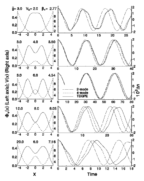
Figure 6: Left column: The functions $\Phi_{+}(x)$ and potentials $V(x)$ for conditions indicated above each frame: $\bar{g},V_{b}$, with $\sigma_{z}$ = 1.5 in each case. The last figure gives the chemical potential, $\beta_{+}$. Right column: time evolution of the fractional number difference, $\Delta n$ times $10^{3}$ for very small initial imbalance. The three curves are obtained from the 2-mode VTM model (long dashes), the 4-mode model (short dashes) and the TDGPE (solid curve).

II.5 Phase space dynamics

The evolution of $z,\phi$ from the coupled equations, (II.2), closely resembles the dynamical evolution phenomena thoroughly discussed in Raghavan . We give a brief review to point out the differences arising from use of the VTM.

To visualize the dynamics, it is helpful to view a plot of the Hamiltonian surface, $H(z,\phi)$, as shown in Fig. 7 for generic values of $A,B$ and $C$. The surface is periodic in $\phi$, with minima at $z=0,\phi=2n\pi$ and saddle points or maxima at $z=0,\phi=(2n+1)\pi$, where $n$ is an integer. Trajectories are horizontal curves (constant $H$) lying on this surface.

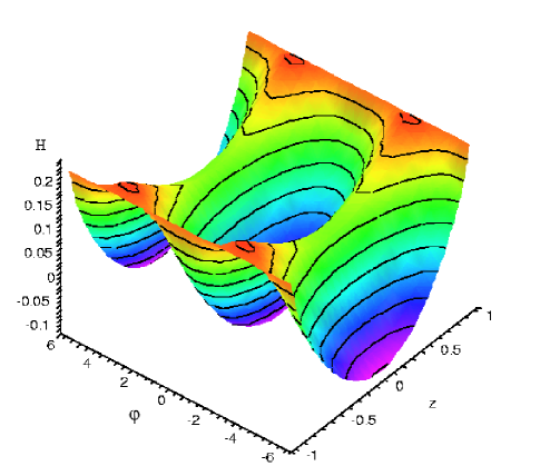
Figure 7: Hamiltonian surface $H(z,\phi)$ for $V_{0}=4$, $\sigma=1.5$, $\bar{g}=1$. Trajectories lie on the surface, following contour lines that represent constant energy levels.

Within either two-mode model, self trapping occurs for $H$ above $H_{s}$, the value of classical Hamiltonian at the saddle point. Critical values of $z=z_{c}$ are defined as values of $z(\phi=2n\pi)=z_{0}$ that give $H(z,\phi)$ equal to $H_{s}$. For $|z_{0}|>z_{c}$, trajectories will not pass through $z=0$ and $z$ will remain positive or negative. For the VTM model, the Hamiltonian given by (16), gives

$$H_{s}=H(0,\pi)=B+\frac{C}{2}=H(z_{c},0).$$ (31)

From this result and (16), we obtain

$$z_{c,V}=\frac{2}{A-C}\left[B(A-B-C)\right]^{1/2}.$$ (32)

For the CTM model, the Hamiltonian of (24) yields

$$H_{s}=H(0,\pi)=2{\cal K}=H(z_{c},0),$$ (33)

so that

$$z_{c,C}=\frac{2}{U}[2{\cal K}(U-2{\cal K})]^{1/2}.$$ (34)

Here the model breaks down when either ${\cal K}<0$ (see Fig. 4) or $U-2{\cal K}<0$.

Before presenting results of calculations of $z_{c}$, we recognize that as $|z|\approx|\Delta n|$ and $\bar{g}$ increase, as in Fig. 6, higher modes enter. The variation of $\Delta n$ with time becomes irregular rather than close to sinusoidal, as shown by several plots obtained from calculations with the TDGPE in Fig. 8. For Fig. 8a and 8b (differing very slightly in $\Delta n(0)$, but on opposite sides of $\Delta n=z_{c}$), closely resemble results one would expect from a two-mode model. Figure 8c and d show irregular curves from the TDGPE in a regime where the two-mode model does not apply. In Fig. 8c, there are oscillations of $\Delta n$ within the range $\Delta n>0$ before $\Delta n$ eventually becomes $<0$. Fig. 8d shows that $\Delta n<0$ is achieved for only a brief duration (between T = 25 and 29). Neither of these cases can be considered “self-trapping,” but they are far removed from symmetric, periodic oscillations. Under such conditions of low barrier and/or strong interactions, it is somewhat arbitrary to make the distinction between self-trapping and not self-trapping.

Nonetheless, we have attempted to establish criteria and apply them consistently so as to compare results from the CTM, VTM, and TDGPE approaches, as shown in Fig. 9. Here, $z_{c}$ values from (32) and (34) have been restated in terms of $\Delta n_{c}$ using (10) in order to compare with TDGPE results. For both $\bar{g}$ = 3.0 and 10.0, when $V_{b}$ is high enough, there is good agreement between VTM and TDGPE results. CTM results are significantly lower for $\bar{g}$=3.0, while for $\bar{g}$=10.0, as in Fig. 3, the fact that ${\cal K}$ becomes negative invalidates this approach in this regime of strong interactions.

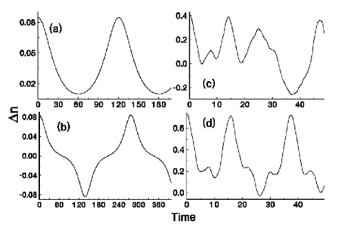
Figure 8: Temporal evolution of $\Delta n$ for various cases: (a) $\bar{g}=3.0,V_{b}=9.0,z_{0}=\Delta n(0)=0.0846$; (b) $\bar{g}=3.0,V_{b}=9.0,\Delta n(0)=0.0838$; (c) $\bar{g}=10.0,V_{b}=5.5,\Delta n(0)=0.411$; (d) $\bar{g}=3.0,V_{b}=4.0,\Delta n(0)=0.735$.

Figure 9: Values for $\Delta n_{c}$ from the CTM, VTM and TDGPE models, for a) $\bar{g}$ = 3.0 and b) $\bar{g}$ = 10.0. The inset in (a) shows the ratio of CTM and VTM values to TDGPE results.

In the self-trapping regime, maximal and minimal values of $z(t)$ can be obtained by solving the equation $\dot{z}=0$:

$$z=\pm\sqrt{1-\left[\frac{|B|}{C-A}\pm\sqrt{\left(\frac{B}{C-A}\right)^{2}-\frac{2H-A}{C-A}}\right]^{2}}.$$ (35)

Plus or minus signs in front of the square root correspond to different initial conditions for $z$ (positive or negative respectively). An elegant discussion of dynamics, and separatrices, in phase space is given in Fran (explicitly for the case $C$=0).

In Raghavan , it was pointed out that closed trajectories on the surface of $H$ can also occur around maxima on the lines $\phi=(2n+1)\pi$. These are the so-called $\pi$-phase modes. For the VTM, the condition for these maxima is that $|B|<|(A+C)|$. The actual values, $z_{\pi}$, at which these maxima occur can vary drastically from one model to the other.

Even for the case of negligibly small overlap, the momentum $z(t)$ in the VTM differs drastically from the CTM when conditions place these two models on opposite sides of the transition to self-trapping. Far from the neighbourhood of the self trapping transition in $\bar{g},\sigma,V_{0}$, the differences are less.

II.6 Second Quantization

Previous discussions of quantized versions of the Bose double well problem Milburn ; Ivanov were valid to first order in the overlap of the wavefunctions in each well. Also in the recent work Mahmud2 , certain approximations are made for the wavefunction overlap. Now that we have a mechanism for treating the overlap more exactly, there are new possibilities for extending the regime of validity of quantum approaches, which are necessarily based on two-mode models.

The energy functional describing trapped BEC in terms of creation and annihilation operators $\psi(x,t)$, $\psi^{\dagger}(x,t)$ can be written

$$H_{2}=H_{0}+H_{1};\ \ \ H_{0} = \int dx\left[-\frac{1}{2}\hat{\psi}^{\dagger}\nabla^{2}\hat{\psi}+\hat{\psi}^{\dagger}V_{ext}\hat{\psi}\right];$$

$$H_{1} = \frac{g}{2}\int dx\hat{\psi}^{\dagger}\hat{\psi}^{\dagger}\hat{\psi}\hat{\psi},$$ (36)

with the commutator $[\hat{\psi}(x,t),\hat{\psi}^{\dagger}(x^{\prime},t)]=\delta(x-x^{\prime})$.

As above, we will characterize the time evolution in terms of two modes that are predominantly (but not exclusively) located in the left and right wells. However, the derivation is easier when written in terms of the symmetric and antisymmetric functions, $\Phi_{\pm}$ rather than in terms of $\Phi_{1,2}$, because $\langle\Phi_{\pm}^{3}\Phi_{\mp}\rangle=0$, whereas $\langle\Phi_{1,2}^{3}\Phi_{2,1}\rangle\neq 0$. We therefore write a “mixed basis” expression:

$$\hat{\psi}=\frac{1}{\sqrt{2}}\left[\hat{c}_{1}(\Phi_{+}+\Phi_{-})+\hat{c}_{2}(\Phi_{+}-\Phi_{-})\right],$$ (37)

in which

$$\hat{c}_{1,2}=\frac{1}{\sqrt{2}}\int dx\hat{\psi}(\Phi_{+}\pm\Phi_{-})$$ (38)

are projections of $\hat{\psi}$. $\Phi_{\pm}$ are solutions to the GP equation as above. In particular, the following form will be useful:

$$-\frac{1}{2}\nabla^{2}\Phi_{i}+V_{ext}\Phi_{i}=\beta_{i}\Phi_{i}-gN|\Phi_{i}|^{2}|\Phi_{i}.$$ (39)

Also we have $[\hat{c}_{i},\hat{c}^{\dagger}_{j}]=\delta_{ij}.$

Substituting 37 and 39 into the above equation for $H_{0}$, we obtain four terms:

$$H_{0}=\frac{1}{2}\left\{\left[\hat{c}_{1}^{\dagger}\hat{c}_{1}+\hat{c}_{2}^{\dagger}\hat{c}_{2}\right]\left[\beta_{+}-\gamma_{++}+\beta_{-}-\gamma_{--}\right]\right.$$

$$\left.+\left[\hat{c}_{1}^{\dagger}\hat{c}_{2}+\hat{c}_{2}^{\dagger}\hat{c}_{1}\right]\left[\beta_{+}-\gamma_{++}-\beta_{-}+\gamma_{--}\right]\right\}$$ (40)

Upon substituting 37 into the above equation for $H_{1}$, we obtain 16 terms, each with products of two creation and two annihilation operators, times integrals of the form

$$(+)^{i}(-)^{j}=\frac{g}{2}\int dx(\Phi_{+}+\Phi_{-})^{i}(\Phi_{+}-\Phi_{-})^{j}.$$ (41)

In particular

$$H_{1}=\hat{c}_{1}^{\dagger}\hat{c}_{1}^{\dagger}\hat{c}_{1}\hat{c}_{1}(+)^{4}+\hat{c}_{2}^{\dagger}\hat{c}_{2}^{\dagger}\hat{c}_{2}\hat{c}_{2}(-)^{4}\hskip 56.9055pt$$ (42)

$$+\left[\hat{c}_{1}^{\dagger}\hat{c}_{1}^{\dagger}\hat{c}_{1}\hat{c}_{2}+\hat{c}_{1}^{\dagger}\hat{c}_{1}^{\dagger}\hat{c}_{2}\hat{c}_{1}+\hat{c}_{1}^{\dagger}\hat{c}_{2}^{\dagger}\hat{c}_{1}\hat{c}_{1}+\hat{c}_{2}^{\dagger}\hat{c}_{1}^{\dagger}\hat{c}_{1}\hat{c}_{1}\right](+)^{3}(-)$$

$$+\left[\hat{c}_{2}^{\dagger}\hat{c}_{1}^{\dagger}\hat{c}_{1}\hat{c}_{2}+\hat{c}_{2}^{\dagger}\hat{c}_{1}^{\dagger}\hat{c}_{2}\hat{c}_{1}+\hat{c}_{2}^{\dagger}\hat{c}_{2}^{\dagger}\hat{c}_{1}\hat{c}_{1}\right.\hskip 56.9055pt$$

$$\left.+\hat{c}_{1}^{\dagger}\hat{c}_{2}^{\dagger}\hat{c}_{1}\hat{c}_{2}+\hat{c}_{1}^{\dagger}\hat{c}_{2}^{\dagger}\hat{c}_{2}\hat{c}_{1}+\hat{c}_{1}^{\dagger}\hat{c}_{1}^{\dagger}\hat{c}_{2}\hat{c}_{2}\right](+)^{2}(-)^{2}$$

$$+\left[\hat{c}_{2}^{\dagger}\hat{c}_{2}^{\dagger}\hat{c}_{1}\hat{c}_{2}+\hat{c}_{2}^{\dagger}\hat{c}_{2}^{\dagger}\hat{c}_{2}\hat{c}_{1}+\hat{c}_{2}^{\dagger}\hat{c}_{1}^{\dagger}\hat{c}_{2}\hat{c}_{2}+\hat{c}_{1}^{\dagger}\hat{c}_{2}^{\dagger}\hat{c}_{2}\hat{c}_{2}\right](+)(-)^{3}$$

$$=\sum_{i=0}^{4}D(i)(+)^{4-i}(-)^{i}\hskip 56.9055pt$$ (43)

Recalling the definitions

$$4U=\gamma_{++}+6\gamma_{+-}+\gamma_{--};\ \ \ 4C=\gamma_{++}+\gamma_{--}-2\gamma_{+-};$$

$$A=U-2C;\ \ \ \Delta\gamma=\gamma_{--}-\gamma_{++};\ \ \ \Delta\beta=\beta_{--}-\beta_{++},$$ (44)

we obtain

$$(\pm)^{4} = \frac{g}{2}\int dx(\Phi_{+}\pm\Phi_{-})^{4}$$ (45)

$$= \frac{1}{2N}(\gamma_{++}+6\gamma_{+-}+\gamma_{--})=\frac{2U}{N};$$

$$(\pm)^{3}(\mp) = \frac{g}{2}\int dx(\Phi_{+}^{2}-\Phi_{-}^{2})(\Phi_{+}^{2}\pm 2\Phi_{+}\Phi_{-}+\Phi_{-}^{2})$$

$$= \frac{1}{2N}(\gamma_{++}-\gamma_{--})=-\frac{1}{2N}\Delta\gamma.$$

$$(+)^{2}(-)^{2} = \frac{g}{2}\int dx(\Phi_{+}^{2}-\Phi_{-}^{2})^{2}$$ (46)

$$= \frac{1}{2N}(\gamma_{++}-2\gamma_{+-}+\gamma_{--})=\frac{2C}{N}.$$

We wish to represent $H_{2}$ in terms of the following operators:

$$N=N_{1}+N_{2}=\hat{c}_{1}^{\dagger}\hat{c}_{1}+\hat{c}_{2}^{\dagger}\hat{c}_{2};\ \ \ J_{x}=\frac{1}{2}(c_{2}^{\dagger}\hat{c}_{2}-c_{1}^{\dagger}\hat{c}_{1})$$

$$J_{y}=\frac{i}{2}(c_{2}^{\dagger}\hat{c}_{1}-c_{1}^{\dagger}\hat{c}_{2});\ \ \ J_{z}=\frac{1}{2}(c_{2}^{\dagger}\hat{c}_{1}+c_{1}^{\dagger}\hat{c}_{2}),$$ (47)

and Casimir element $J^{2}=\frac{\hat{N}}{2}\left(\frac{\hat{N}}{2}+1\right)$, so that

$$[J_{i},J_{j}]=i\epsilon_{ijk}J_{k}.$$ (48)

Also we will need

$$N_{1}N_{2}=\frac{N^{2}}{4}-J_{x}^{2}.$$ (49)

Then the products of four annihilation and creation operators, the $D(i)$ terms in (42), reduce to:

$$D(0)+D(4)=(\hat{c}_{1}^{\dagger})^{2}\hat{c}_{1}^{2}+(\hat{c}_{2}^{\dagger})^{2}\hat{c}_{2}^{2}=\frac{N^{2}}{2}-N+2J_{x}^{2};$$

$$D(1)+D(3)=4(N-1)J_{z};\hskip 56.9055pt$$

$$D(2)=4J_{z}^{2}+2N_{1}N_{2}=4J_{z}^{2}+\frac{N^{2}}{2}-2J_{x}^{2}.$$ (50)

Collecting terms, neglecting terms that are constant, we obtain

$$H_{2}=-J_{z}\left(\Delta\beta+\Delta\gamma-\frac{2\Delta\gamma}{N}\right)+\frac{4(A+C)}{N}J_{x}^{2}+\frac{8C}{N}J_{z}^{2}.$$ (51)

The quantum equations of motion read

$$\dot{J_{i}}=i[\hat{H},J_{i}],$$ (52)

which yields

$$\dot{J_{x}} = \left(\Delta\beta+\Delta\gamma-\frac{2\Delta\gamma}{N}\right)J_{y}-\frac{8C}{N}(J_{y}J_{z}+J_{z}J_{y})$$

$$\dot{J_{y}} = -\left(\Delta\beta+\Delta\gamma-\frac{2\Delta\gamma}{N}\right)J_{x}$$

$$-\frac{8C}{N}(J_{x}J_{z}+J_{z}J_{x})-\frac{4(A+C)}{N}(J_{z}J_{x}+J_{x}J_{z})$$

$$\dot{J_{z}} = \frac{4(A+C)}{N}(J_{y}J_{z}+J_{z}J_{y})$$ (53)

The above Hamiltonian, $H_{2}$, is to be compared with expressions derived previously Milburn ; Ivanov ; Leggett ; Links ; Fran ; Mahmud2 . Although a general second quantized Hamiltonian was written many years ago by nuclear physicists LKM (since known as the LMG model), most applications seem to involve simply the terms in $J_{z}$ and $J_{x}^{2}$. Using the operators defined above and assuming a symmetric double well potential, the expression in Leggett , for example, can be written:

$$H_{\rm canon}=-{\cal E}_{J}J_{z}+\frac{1}{2}KJ_{x}^{2}.$$ (54)

The comparison provides the following translation:

$${\cal E}_{J}=\Delta\beta+\Delta\gamma-\frac{2\Delta\gamma}{N};\ \ \ K=\frac{8(A+C)}{N}.$$ (55)

The regimes defined in Leggett then become (neglecting the $2\Delta\gamma/N$ term:

$${\rm Rabi} : \ \frac{K}{{\cal E}_{J}}\ll\frac{1}{N}\Rightarrow R\ll 1;\ \ \ R=\frac{8(A+C)}{\Delta\beta+\Delta\gamma};$$

$${\rm Josephson} : \ \ \frac{1}{N}\ll\frac{K}{{\cal E}_{J}}\ll N\Rightarrow 1\ll R\ll N^{2};$$

$${\rm Fock} : \ \ N\ll\frac{K}{{\cal E}_{J}}\Rightarrow N^{2}\ll R.$$ (56)

Thus for the second-quantized version as for the first-quantum GP equation version discussed above, we have obtained a Hamiltonian with a form similar to those previously derived, but with slightly different parameters, and with extra terms that may be important for large atom-atom interactions.

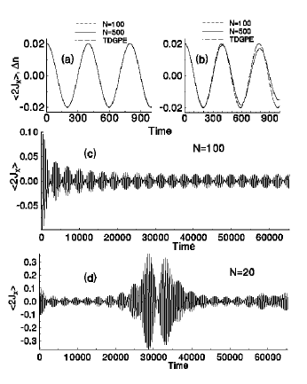
Figure 10: In the limit of small $\bar{g}$ and small times, the temporal behavior of $2\langle J_{x}\rangle$ and $\Delta n(t)$ approach each other. All of these plots are for $\sigma=1.5,V_{b}$=6.0. (a) $\bar{g}$ = 1.0 $\times 10^{-4}$, $R$ = 0.017; (b-d) $\bar{g}=1.0\times 10^{-3}$, $R$ = 0.17. For (a) and (b), the quantum and classical periods are nearly the same, but (b) begins to show a decrease of oscillation amplitude in the quantum case, due to the second term in $H_{2}$. This modulation of the oscillations is shown over longer time in (c), for $N$=100, and in (d), for $N$=20.

Our formulation provides a connection with experimental conditions through the Gross-Pitaevskii equation. The expectation value $\langle 2J_{x}\rangle$ describes the difference between the number of particles in the two modes, and is therefore an analog of the classical quantities, momentum, $z(t)$, and number difference, $\Delta n(t)$. The connection between $\langle 2J_{x}\rangle$ and $\Delta n(t)$ can be most easily seen in the limit of very small interactions (small $\bar{g}$), which is essentially the “Rabi regime” as defined in Leggett and above. The following conclusions are based simply on an empirical evaluation of numerical results.

For $\bar{g}<10^{-2}$, there are clear tunneling oscillations with frequency $\Delta\beta$ from the first term in $H_{2}$ ($\Delta\gamma\ll\Delta\beta$ here). These oscillations are modulated by effects from the second term (in $J_{x}^{2}$) in $H_{2}$, which increase with $\bar{g}$. For constant $\bar{g}=gN$, these modulations are independent of $N$ over a large range of $N$, but undergo an additional modulation whose period decreases with $N$, as shown in Fig. 10. This suggests that there are various orders of time-dependent perturbations by which the second term in $H_{2}$ perturbs the effect of the first. However, we have not been able to produce a quantitative perturbation-theoretic model. For long enough times, one observes the collapse and revival effects noted in Milburn and shown in Fig. 11. For larger values of $\bar{g}$, these structures no longer persist.

Since it has been difficult to experimentally observe even a single oscillation, and since it is difficult to control $N$ and the initial imbalance, these oscillatory patterns may be impossible to observe. We do find however, that the collapse and revival structure can persist even if there is a spread of initial values of $N_{1}-N_{2}$. Figure 11 compares results for fixed $N$=30, for an initial sharp $N_{1}$ distribution, $N_{1}=27$, with results for an initial flat distribution over the range $24\leq N_{1}\leq 30$. The stability of a part of the revival structure may occur because two parameters are needed to characterize a point on the sphere that is isomorphic to the $SU(2)$ algebra used above. More extensive numerical results of phase space oscillations are given in Links , and detailed studies of averages in phase space using the Husimi distribution have been presented in Mahmud2 .

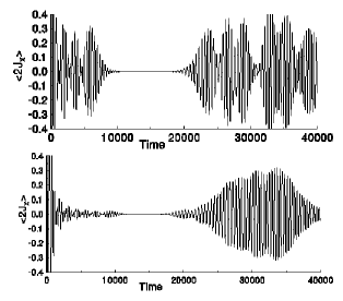
Figure 11: Collapse and revivals for $\bar{g}$=3.0$\times 10^{-3}$, $R$=0.50, for precisely defined $N=30$, but in (a) for precisely defined $N_{1}=27$ and in (b) for a flat distribution $24\leq N_{1}\leq 30$.

III Calculations in 3D

III.1 General Formalism

In comparing with experimental results, the transverse confinement enters. In this study, we consider moderate transverse confinement, not approaching the Tonks-Girardeau regime MO . We have extended the above methods to 3D as follows. We write the TDGPE first in MKS units, denoted by overbars:

$$i\hbar\frac{\partial\bar{\psi}}{\partial\bar{t}}=\left[-\frac{\hbar^{2}}{2m}\bar{\nabla}^{2}+\frac{m}{2}\sum_{i}\omega_{i}^{2}\bar{x}_{i}^{2}\right.\hskip 85.35826pt$$

$$\left.+V_{B}+g_{3D}|\bar{\psi}(\bar{\bf x},t)|^{2}\right]\bar{\psi}(\bar{\bf x},t)\hskip 42.67912pt$$ (57)

where $m$ is the atomic mass, and $g_{3D}=4\pi\hbar^{2}a_{3D}/m$, $a_{3D}$ is the 3D scattering length, and $\int d{\bf\bar{x}}|\bar{\psi}({\bf\bar{x}})|^{2}=N$. The external potentials of interest here will include a purely harmonic term as given above, plus a barrier term as a function of $z$ that will be chosen to be Gaussian or proportional to a $\cos^{2}$ function, as in the experiments of Albiez .

We let

$$\omega_{x}=\omega_{y}=\eta\omega_{z},$$ (58)

and scale the coordinates and time as

$$\bar{x}_{i}=\alpha_{i}x_{i};\ \ \alpha_{i}^{2}=\hbar/m\omega_{i};\ \ \bar{t}=t/\omega_{z}.$$ (59)

Then since

$$\int\!d{\bf x}|\psi(x)|^{2}\!=\!N=\!\!\int\!\!d{\bf\bar{x}}|\bar{\psi}(\bar{\bf x})|^{2}\!=\!\alpha_{x}\alpha_{y}\alpha_{z}\!\!\int\!d{\bf x}|\bar{\psi}({\bf x})|^{2},$$ (60)

$\bar{\psi}=(\alpha_{x}\alpha_{y}\alpha_{z})^{-1/2}\psi$, and (III.1) becomes

$$i\frac{\partial\psi(x,y,z,t)}{\partial t}={\cal H}(\lambda,\psi)\psi(x,y,z,t):\hskip 71.13188pt$$

$${\cal H}(\lambda,\psi)=-\frac{\eta}{2}\left(\frac{\partial^{2}}{\partial x^{2}}+\frac{\partial^{2}}{\partial y^{2}}\right)-\frac{1}{2}\frac{\partial^{2}}{\partial z^{2}}+\frac{\eta}{2}(x^{2}\!+\!y^{2})$$

$$+\frac{z^{2}}{2}+V_{B}+4\pi\eta\left(\frac{a_{3D}}{\alpha_{z}}\right)|\psi(x,y,z,t)|^{2}\hskip 14.22636pt$$ (61)

where $\lambda$ represents the arguments $\eta,V_{B},N,a_{3D}$ and $\alpha_{z}$.

An ansatz analogous to (2) can now be introduced:

$$\psi({\bf x},t) = \sqrt{N}[\psi_{1}(t)\Phi_{1}({\bf x})+\psi_{2}(t)\Phi_{2}({\bf x})];$$ (62)

$$\Phi_{1,2}({\bf x}) = \frac{\Phi_{+}({\bf x})\pm\Phi_{-}({\bf x})}{\sqrt{2}},$$ (63)

where

$$\Phi_{\pm}(x,y,z)=\pm\Phi_{\pm}(x,y,-z);\ \ \int dxdydz\Phi_{\pm}^{2}=1.$$ (64)

The stationary GP equations take the form:

$$\beta_{\pm}\Phi_{\pm}(x,y,z)={\cal H}(\lambda,\Phi_{\pm})\Phi_{\pm}(x,y,z).$$ (65)

Because the transverse wavefunction is very nearly Gaussian, some authors have simply assumed a Gaussian, possibly with a $z$-dependent width, and obtained modified equations Salasnich ; Das for what we have called $\psi_{1}(z)$. Because we wanted to consider cases where the Gaussian form may not be valid, we used general 3D algorithms. Initial $\Phi_{\pm}$ wavefunctions were obtained by diagonalizing the DVR Hamiltonian DVR1 using sparse matrix techniqes Davidson , which made calculations with $>$120,000 mesh points possible in minutes on a PC. To calculate the time evolution, the split-operator method Feit with Fast Fourier transform FF was used, requiring an hour or more of $\approx$2 GHz CPU time, in view of the small time steps required.

From the $\Phi_{\pm}$ functions calculated from the 3D time-independent Gross-Pitaevskii equation, one can also obtain the parameters $\beta_{\pm},\gamma_{i,j}$, $A,B$ and $C$ as in Section II, to provide a two-mode representation of tunneling oscillations in 3D. In translating results from 1D to 3D for $g_{1D}=g_{3D}=4\pi\eta a_{3D}/\alpha_{z}$, we find that, in the limit of weak interactions and $\eta\geq 1$, the $\gamma_{ij}$ functions for 3D are a factor of $2\pi$ smaller than the corresponding 1D $\gamma_{ij}$ functions. The explanation touches on the basic properties of tight transverse confinement.

If the transverse confinement is symmetric in $x$ and $y$ and is tight enough, the 3D wavefunction $\Phi_{+}(x,y,z)$ can be factored into a function of $z$ and a function of $\rho=\sqrt{(x^{2}+y^{2})}$. Then if also the interactions are weak enough, the $\rho$ function will be a Gaussian:

$$\Phi_{+}(x,y,z)=\Phi_{+}(\rho,z)=e^{-\rho^{2}/2}\phi_{1}(z).$$ (66)

The normalization condition is

$$1=\int dxdydz\Phi_{+}(x,y,z)^{2}\hskip 71.13188pt$$

$$=2\pi\int d\rho\rho e^{-\rho^{2}}\int dz\phi_{1}(z)^{2}=\pi\int dz\phi_{1}(z)^{2}.$$ (67)

Under the above conditions, and if $g_{1D}=g_{3D}$, then to within a constant of proportionality, $\phi_{1}(z)$ will also be a solution of the 1D problem: $\phi_{1}(z)\propto\Phi_{+}^{1D}(z)$. For the 1D problem, $\int dz|\Phi_{+}^{1D}(z)|^{2}=1$, so from the different normalizations, we see that, under all the above stated conditions,

$$\phi_{1}(z)=\frac{1}{\sqrt{\pi}}\Phi_{+}^{1D}(z).$$ (68)

The 3D version of $\gamma_{++}$ becomes

$$\gamma_{++}^{3D}=\int dxdydz|\Phi_{+}^{3D}|^{4}\hskip 71.13188pt$$

$$=2\pi\int\!\rho d\rho e^{-2\rho^{2}}\int\!dz\phi_{1}(z)^{4}=2\pi\frac{1}{4}\frac{\gamma_{++}^{1D}}{\pi^{2}}=\frac{\gamma_{++}^{1D}}{2\pi}.$$ (69)

Similar relations hold also for $\gamma_{--}^{3D}$ and $\gamma_{+-}^{3D}$. For larger interactions, the $\rho$ dependence is not exactly Gaussian, the functions $\Phi_{\pm}^{3D}$ no longer factorize, and the parameters $\gamma_{ij}^{3D}$ deviate from the above relations. Figure 12 shows plots of $\gamma_{++},\gamma_{--}$ and $\gamma_{+-}$ from 3D calculations with $\eta$ = 1 and 100, as compared with 1D results. For $\eta$=100, the wavefunction is more concentrated than for $\eta=1$, so the values for $\gamma_{ij}$ are slightly larger. Each is 5 to 6 times smaller than for the 3D case. Otherwise the dependences on $V_{b}$ are very similar.

Figure 12: Values for $\gamma_{ij},i,j=+,-$ from 3D calculations with $\eta$=1 and 100 (left axis), as compared with a 1D calculation (right axis). Solid lines denote $\gamma_{++}$, short dashes $\gamma_{+-}$, and longer dashes $\gamma_{--}$. For 3D, the $\gamma_{ij}$ are approximately $2\pi$ larger than for 1D.

There are other differences between 3D and 1D properties. The difference energy, $\Delta\beta$, and hence also the parameter $B$ decrease more rapidly as a function of barrier height. Figure 13 compares the parameters $A,B$ and $C$ in 3D ($\eta=1$) and in 1D, for the case $\bar{g}=10$. Evidently, finite transverse confinement decreases the difference between the symmetric and antisymmetric condensate energies. The differences are much the same for $\eta$ =100 as for $\eta$=1. Also for $\eta=1$ $\bar{g}$=10, Fig. 13b shows that the plasma oscillation frequency in the limit of small $z,\phi$, for barrier height, $V_{b}>5$, is even less than a factor of $2\pi$ smaller in 3D than in 1D. This statement has been found to be true for $\eta$=1 and 100, and $\bar{g}$ up to 10.

We conclude that two-mode models tend to be even more valid in 3D than in 1D.

Figure 13: (a) A comparison of calculated values for the parameters $A,B$ and $C$ for 1D and for 3D, for $\eta=1$ and $\bar{g}$=10. (b) A comparison of Josephson plasma oscillation frequencies, $\omega_{0}$, for 1D and 3D, also for $\eta=1$ and $\bar{g}$=10.

Linear combinations of $\Phi_{\pm}$ functions provide the initial condition for the TDGPE, for which we use the split operator approach with fast Fourier transform Feit ; FF . To be able to compare TDGPE results with (II.3), we use a very small initial imbalance ($z_{0}$ =0.002) for the TDGPE calculations. For the two-mode models, parameters are obtained from wavefunctions calculated with the time-independent 3D GP equation, as for 1D results above. The results for $\omega_{o}$ are shown in Fig. 14a-c. (Fig. 14d pertains to the experiments of Albiez as discussed below). The plasma oscillation frequency obtained from the TDGPE increases rapidly beyond $\bar{g}=gN\approx$ 3. The two-mode model results match the TDGPE results well for $\bar{g}<1$. Fig. 14a, for Gaussian barrier of height $V_{b}=5\hbar\omega_{z}$, shows good agreement for both the VTM and CTM with TDGPE results, up to $\bar{g}$ = 100. On the other hand, when the barrier height is raised to 8$\hbar\omega_{z}$, the CTM fails for $\bar{g}>30$, for both $\eta=1$ (b) and $\eta=100$ (c). For the latter, the VTM result begins to deviate significantly from the TDGPE value around $\bar{g}$=100. The failure of the CTM here is analogous to the situation shown in Fig. 3, and occurs because ${\cal K}$ becomes negative.

Figure 14: Josephson plasma oscillation frequencies calculated from the TDGPE and from VTM and CTM models, using (II.3) and the $\beta_{\pm},\epsilon_{\pm}$ and $\gamma_{\pm}$ parameters obtained from the 3D wavefunctions, $\Phi_{\pm}$. For (a-c), Gaussian barriers were used, as all the 1D calculations. For (d), a $\cos^{2}$ function to reproduce the barrier in Albiez . Other parameters were (a) $\eta$=1.0; $V_{b}$=5.0; (b) $\eta=1.0,V_{b}=8.0$; (c) $\eta=100,V_{b}=8.0$; (d) Corresponding closely to the experiments in Albiez (see text), $\nu_{x}$ = 66 Hz, $\nu_{y}$ = 90 Hz, $\nu_{z}$ = 78 Hz, barrier $V_{b}$ = 5.28 $\hbar\omega_{z}$ times the cos² function given in the text. The values plotted are for $z_{0}=0.28$ as in the experiments, rather than for the limiting case of small $z,\phi$, hence are labeled $\omega$ rather than $\omega_{0}$.

III.2 Comparison with Recent Experiments

Very recently, the first quantitative experimental observations of oscillations of Bose condensates in a double well potential have been performed Albiez . The harmonic confinement was created by overlapping tightly focussed Gaussian laser beams. The harmonic frequencies were 66, 90 and 78 Hz in what we will call the $x,y$ and $z$ directions. To produce the double well, an optical standing wave from two beams of wavelength 811 nm, at an angle of 9^o were added, producing a barrier of the form $V_{b}\cos(z\pi/w)^{2}$, with $V_{b}=$ 413(20) Hz, and $w$ = 5.20(20)$\mu$m. 1150 ⁸⁷Rb atoms were loaded into this trap. We have modeled this experimental configuration and find the effective value of $gN=58.8$ from III.1, which corresponds to $\bar{g}\approx 10$ in 1D simulations.

The reported experimental period of oscillation for $z_{0}=0.28(6)$ was 40(2) msec. Albiez , which corresponds to the value indicated by the large diamond in Fig. (14)d. We obtain values very close to this observed tunneling frequency with both the VTM and TDGPE by using a value for $a_{3D}=100a_{0}$ (where $a_{0}$ is the Bohr radius) Verhaar . For this initial value $z_{0}$, (although not for very small values of $z_{0}$), self-trapping occurs with the CTM model, when based on solutions of the Gross-Pitaevskii equation. The calculated CTM frequency drops rapidly before this point, as shown in Fig. (14)d.

Note that by reference to Figs. 14a-c, we conclude that as long as the temperature is sufficiently low (the temperature for the experiments of Albiez was immeasurably low), the aspect ratio is not important, as results for $\eta=100$ and =1 are very similar, but the relatively large value of the nonlinear term is important in determing the validity of two-mode models.

Using the TDGPE, we have calculated a value of $z_{c}$=0.39 for the stated conditions of these experiments, which is consistent with the observed oscillations at $z_{0}=0.28(6)$ and self-trapping for $z(0)=0.62(6)$, but lower than the value of $z_{c}$ = 0.50(5) quoted in Albiez . In this paper, the authors performed calculations with the transverse Gaussian model of Salasnich and obtained good agreement with experimental observations. Our contribution is simply to show that a two-mode model, with parameters from GP eigenfunctions, also comes quite close to reproducing the experimental observations.

The other experiments that helped to motivate this study were performed at NIST, MD, with ⁸⁷Rb atoms in a “pattern-loaded” optical lattice. The atoms were first loaded into a coarse lattice from Bragg-diffracted laser beams, and then a finer lattice was turned on, such that every third lattice site was occupied Peil . We are presently working to develop a modification of the present approach to deal with such phenomena in a periodic lattice.

IV Conclusions

By rigorous solution of coupled equations for the symmetric and anti-symmetric wavefunctions for a Bose condensate in a double well potential, we have derived equations for a new two-mode model that provides for variation of the tunneling parameter with time, depending on the differences of number and phase of atoms in the two wells. We have compared results from this “variable tunneling model” (VTM) with results from other two-mode models, from multi-mode models that we have constructed, and from solutions of the time-dependent Gross-Pitaevskii equation (TDGPE). In making these comparisons, we numerically compute wavefunctions from the stationary Gross-Pitaevskii equation and use appropriate integrals of these wavefunctions in the model equations. For small values of the non-linear interaction term and moderate potential barriers, all the models agree nicely. When the nonlinear interaction term exceeds a certain value, the tunneling parameter in the usual “constant tunneling model” (CTM) becomes negative, and thus the Josephson plasma oscillation frequency becomes imaginary. The VTM remedies this problem, and produces better agreement with results of the TDGPE. We have performed such comparisons for 1D situations and also for 3D situations, for which we have obtained 3D solutions of the stationary and time-dependent GP equations. The recent experimental observations of tunneling oscillations and macroscopic self-trapping of Albiez are in the regime of moderately strong non-linear interactions because of the large number of atoms (1150 ⁸⁷Rb atoms). Results from both the TDGPE and VTM for the observed tunnelling oscillation frequency are in good agreement with the experimental value. However, under the conditions of the experiment, the CTM when based on parameters from the GP equation, leads to self-trapping rather than oscillation.

We also have applied our approach to derive an improved Hamiltonian for quantum calculations, but find no reliable standards to compare this approach with other quantization approaches. What we have not investigated here are damping effects of thermal excitations, as considered in Zapata and Marino .

We gratefully acknowledge support from NSF Grant PHY0354211, and from the ONR. We are especially indebted to M. Oberthaler for sending a preprint of Albiez before publication. Communications with M. Olshanii, V. Dunjko, H. T. C. Stoof, V. Korepin and D. Averin have been valuable in preparing this report. In addition, we thank A. Muradyan for a critical reading of the manuscript.

References

- (1) B. D. Josephson, Phys. Lett., 1, 251 (1962).
- (2) J. Javanainen, Phys. Rev. Lett. 57, 3164 (1986).
- (3) M. W. Jack, M. J. Collett, and D. F. Walls, Phys. Rev. A, R4625 (1996).
- (4) G.J. Milburn, J. Corney, E. M. Wright, and D. F. Walls, Phys. Rev. A 55 4318 (1997)
- (5) A. Smerzi, S. Fantoni, S. Giovannazzi, and S. R. Shenoy, Phys. Rev. Lett. 79, 4950 (1997).
- (6) I. Zapata, F. Sols and A. J. Leggett, Phys. Rev. A 57, 1208 (1998).
- (7) M. J. Steel and M. J. Collett, Phys. Rev. A 57, 2920 (1998).
- (8) R. W. Spekkens and J. E. Sipe, Phys. Rev. A 59, 3868 (1999).
- (9) J. Javanainen and M. Yu. Ivanov, Phys. Rev. A 60, 2351 (1999).
- (10) S. Raghavan, A. Smerzi, S. Fantoni and S. R. Shenoy, Phys. Rev. A 59, 620 (1999).
- (11) E. Ostrovskaya, Y. Kivshar, M. Lisak, B. Hall, F. Cattani and D. Anderson, Phys. Rev. A 61, 031601 (2000).
- (12) R. Franzosi, V. Penna, R. Zecchina Int. J. Mod. Phys. B 14 943 (2000)
- (13) G.-S. Paraoanu, S. Kohler, F. Sols and A. J. Leggett, J. Phys. B. 34, 4689 (2001).
- (14) A.J. Leggett Rev. Mod. Phys. 73 307 (2001).
- (15) J. Anglin, P. Drummond and A. Smerzi, Phys. Rev. A 64, 063605 (2001).
- (16) K. W. Mahmud, J. N. Kutz and W. P. Reinhardt, Phys. Rev. A 66, 063607 (2002).
- (17) K. W. Mahmud, H. Perry and W. P. Reinhardt, Phys. Rev. A 71, 023615 (2005).
- (18) A. P. Tonel, J. Links, A. Foerster, quant-ph/0408161
- (19) D. V. Averin, A. B. Zorin, K. K. Likharev, Zh. Eksp. Teor. Fiz. 88, 692 (1985) [Sov. Phys. JETP 61, 407 (1985)].
- (20) M. R. Andrews, C. G. Townsend, H.-J. Miesner, D. S. Durfee, D. M. Kurn, and W. Ketterle, Science, 175, 637 (1997).
- (21) F. S. Cataliotti, S. Burger, C. Fort, P. Maddaloni, F. Minardi, A. Trombettoni, A. Smerzi, and M. Inguscio, Science, 293, 843 (2001).
- (22) M. Albiez, R. Gati, J. Fölling, S. Hunsmann, M. Cristiani, and M. K. Oberthaler, cond-mat/0411757 (Dec. 7, 2004).
- (23) S. Peil, J. V. Porto, B. Laburthe Tolra, J. M. Obrecht, B. E. King, M. Subbotin, S. L. Rolston, and W. D. Phillips, Phys. Rev. A 67, 051603(R) (2003).
- (24) H. Ott, J. Fortágh, S. Kraft, A. Günther, D. Komma and C. Zimmerman, Phys. Rev. Lett., 91, 040402 (2003).
- (25) J. Williams et. al. Phys. Rev. A 59 R31. (1999)
- (26) J. Hu, J. Yin J. Opt. Soc. Am. B 19 (2002) 2844.
- (27) P. Hommelhoff, W. Hänsel, T. Steinmetz, T. W. Hänsch, and J. Reichel, New Journal of Physics, 7, 3 (2005).
- (28) D. Jaksch, C. Bruder, J. I. Cirac, C. W. Gardiner, and P. Zoller, Phys. Rev. Lett. 81, 3108 (1998).
- (29) M.P.A. Fisher, P.B. Weichman, G. Grinstein, & D.S. Fisher, Phys. Rev. B 40, 546 (1989).
- (30) A. Trombettoni and A. Smerzi, J. Phys. B 34, 4711 (2001).
- (31) A.-M. Rey, P. B. Blakie and C. W. Clark, Phys. Rev. A 67, 053610 (2003).
- (32) D. Ananikian and T. Bergeman, BAPS, 49 (No. 3), 78 (2004).
- (33) Z. Basic, J.C. Light, J. Chem. Phys, 85, 4594 (1986).
- (34) D.T. Colbert, W.H. Miller, J. Chem. Phys. 96 (3), 1982 (1992).
- (35) H. J. Lipkin, N. Meshkov and A. J. Glick, Nucl. Phys. 62, 188 (1964). We thank Julien Vidal for pointing out this paper to us.
- (36) M. Olshanii, Phys. Rev. Lett. 81, 938 (1998).
- (37) L. Salasnich, A. Parola and L. Reatto, Phys. Rev. A 65, 043614 (2002).
- (38) K. Das, Phys. Rev. A 66, 053612 (2002).
- (39) C. W. Murray, S. C. Racine and E. R. Davidson, J. of Comp. Phys. 103, 382 (1992); E. R. Davidson, Computers in Physics, 7, 519 (1993).
- (40) M. A. Feit, J. A. Fleck, and A. Steiger, J. Comp. Phys., 47, 412 (1982).
- (41) J. W. Cooley and J. W. Tukey, Math. of Comp. 19, 297 (1965).
- (42) E. G. M. van Kempen, S. Kokkelmans, D. Heinzen, and B. J. Verhaar, Phys. Rev. Lett. 88, 093201 (2002).
- (43) I. Marino, S. Raghavan, S. Fantoni, S. R. Shenoy and A. Smerzi, Phys. Rev. A 60, 487 (1999).