Superconducting Fluctuation Corrections to the Thermal Conductivity in Granular Metals

Abstract

The first-order superconducting fluctuation corrections to the thermal conductivity of a granular metal are calculated. A suppression of thermal conductivity proportional to $T_{c}/(T-T_{c})$ is observed in a region not too close to the critical temperature $T_{c}$. As $T\simeq T_{c}$, a saturation of the correction is found, and its sign depends on the ratio between the barrier transparency and the critical temperature. In both regimes, the Wiedemann-Franz law is violated.

I Introduction

In normal metals, in the presence of BCS interaction, electrons can form Cooper pairs even for temperatures $T$ larger than the critical temperature $T_{c}$. As $T\geq T_{c}$, the pairs have a finite lifetime, the Ginzburg-Landau (GL) time, inversely proportional to the distance from the critical temperature $\tau_{GL}\sim\left(T-T_{c}\right)^{-1}$. These superconducting fluctuations strongly affect both the thermodynamic and transport properties and since many years they are widely studied both theoretically and experimentally LV04 .
The first analysis of fluctuation corrections has been performed on electrical conductivity where the pairing leads to three distinct contributions named the Aslamazov-Larkin (AL), the Maki-Thompson (MT) and Density of States (DOS) terms. In the first one, the formation of Cooper pair leads to a parallel superconducting channel in the normal phase; the second takes into account the coherent scattering off impurities of the (interacting) electrons; finally, the third one is due to the rearrangement of the states close to the Fermi energy since electrons involved in pair transport are no longer available for single particle transport. Both the AL and MT terms lead to an enhancement of the conductivity above $T_{c}$, on the contrary, the DOS correction is of opposite sign.
The analysis of superconducting fluctuation corrections to thermal conductivity dates back to the early 1960s, when Schmid S66 and Caroli and Maki CM67 found an expression for the heat current in the framework of the phenomenological time dependent GL theory, (TDGL). More recently, a complete analysis was performed, in the same framework of the TDGL, by UssishkinISS03 . Abrahams et al. ARW70 first pointed out the divergence of the thermal conductivity in the vicinity of the critical temperature due to the opening of the fluctuation pseudogap in the density of states (DOS) energy dependence in the homogeneous case. Niven and Smith have shown NS02 that Abrahams’s DOS correction [$\approx Gi\ln(1/\epsilon)$, $\epsilon=(T-T_{c})/T_{c}$, $Gi$ being the so-called Ginzburg-Levanyuk parameter] is exactly compensated by the regular Maki-Thompson (MT) one; hence, all singular first order fluctuation corrections are cancelled out. The only surviving contribution to heat conductivity, the Aslamazov-Larkin (AL) one, is non-singular in temperature. Therefore, in bulk metals, no singular behaviour of the heat current is expected at the metal-superconductor phase transition.
In this paper we are interested in the superconducting fluctuation corrections to the thermal conductivity in a granular superconductors, an ensemble of metallic grains embedded in an insulating amorphous matrix and undergoing a metal-superconductor phase transition due to the existence of pairing interaction inside each grain. The electrons can diffuse in the system due to tunneling between the grains. Experimentally, this kind of systems have been investigated, for example, in Ref. GER97, . Each Al grain has an average dimension of 120Å, while the sample has a linear dimension of the order of mm, that is, much larger than the superconducting coherence length. The reason for studying thermal transport in granular metals is that, depending on the temperature regime, a radically different behaviour, as compared with the homogeneous case, may emerge. In fact, in granular material (a similar situation occurs in layered superconductors) the AL and MT contributions are of higher order in the tunneling amplitude as compared to the DOS. This effect has been observed, for example, in the electrical BMV93 and the optical conductivity FV96 of layered superconductors and the electrical conductivity BEL00 of granular systems. Indeed, in granular superconductors there is a temperature region in which a singular correction due to superconducting fluctuations for a quasi-zero-dimensional system dominates the behaviour of the thermal conductivity; such a correction can be either negative or positive, depending on the ratio between the barrier transparency and the critical temperature $T_{c}$. When the temperature approaches $T_{c}$, the behaviour observed in homogeneous systems is recovered, and the divergence will be cut off to crossover to the regular behaviour. Moreover, a significant difference with the homogeneous systems is present, the constant correction at $T=T_{c}$ being either negative or positive depending on the above-mentioned ratio. For some choice of the parameter, a non-monotonic temperature dependent behaviour of the correction is possible.
A phenomenological approach to granular superconductors has been proposed long ago P67 ; DIG74 , while the microscopic theory has only been formulated very recently BEL00 ; LV04 . The difference between bulk and granular microscopic theory is mainly based on the renormalization of the superconducting fluctuation propagator due to the presence of tunneling. This renormalization accounts for the possibility that each electron forming the fluctuating Cooper pair tunnels between neighbor grains during the Ginzburg-Landau time.
The paper is organized as follows. In Section II, we describe and formulate the model. Section III contains the main steps and assumptions of the calculation of fluctuation propagator. Its expression, calculated in Ref. BEL00, , is given explicitly at every order in tunneling in the ladder approximation. By means of that, DOS, MT, and AL corrections are evaluated. For each of those corrections, an explicit form for the response function is presented. In the final section, we discuss the overall behaviour of the fluctuation corrections to thermal conductivity as a function of temperature. For temperatures sufficiently far from $T_{c}$, the system behaves as in the zero-dimensional case. In this region, the correction to the heat conductivity has a singular behaviour: $\left|\delta\kappa\right|\propto\kappa_{0}/\left({g_{T}}\epsilon\right)\;$, where $\kappa_{0}$ is the classical Drude conductivity for a granular metal, and it reads

$$\kappa_{0}=\frac{8\pi}{3}g_{T}a^{2-d}T\;,$$ (1)

$a$ being the size of a single grain, $d$ the dimensionality of the system and $\epsilon=\left(T-T_{c}\right)/T_{c}$ the reduced temperature. We defined the dimensionless macroscopic tunneling conductance $g_{T}=\left[(\pi/2)t\nu_{F}\right]^{2}$, with $\nu_{F}$ the electronic density of states at the Fermi level, and $t$ the hopping energy. On the other hand, when the correlation length increases until the distance between two nearest neighbor grains, the tunneling becomes important and the correction, exactly at the critical temperature, reduces to a constant

$$\delta\kappa=\frac{1}{zg_{T}}\left(\frac{9}{2\pi}\frac{g_{T}\delta}{T_{c}}-\frac{3}{\pi^{2}}\right){\kappa_{0}}.$$ (2)

Connections with the homogeneous metal results are discussed. In the appendix, we briefly review the evaluation of the superconducting fluctuation propagator in a granular metal. Throughout the paper, we set $\hbar=k_{B}=1$.

II The model

We consider a $d-$dimensional array of metallic grains embedded in an insulating amorphous matrix, with impurities on the surface and inside each grain. Even if the analytical model we use is for a perfectly ordered $d$-dimensional matrix, the results we found still hold for an amorphous one. Indeed, one can imagine different possible configurations of spatial position of grains in the lattice, that is, different disordered configurations. Consequentely, the hopping matrix shall vary for each sample. By performing the average over disorder, one gets a model with the same value of coordination number and hopping energy, $t$, for different configurations. In other words, our description is correct until the system can be described by a dimensionless tunneling conductance, $g_{T}$, on a scale which is much bigger than the typical linear dimension of the grains, $a$, but smaller than the macroscopic dimension of the whole sample.
The Hamiltonian of the system reads

$$\hat{H}=\hat{H}_{0}+\hat{H}_{P}+\hat{H}_{T}\;.$$ (3)

$\hat{H}_{0}$ and $\hat{H}_{P}$ describe the free electron gas and the pairing Hamiltonian inside each grain, respectively

$$\hat{H}_{0} = \sum_{i,k}\varepsilon_{i,k}\hat{a}^{\dagger}_{i,k}\hat{a}_{i,k}+\hat{H}_{\mathrm{imp}}\;,$$ (4)

$$\hat{H}_{P} = -\lambda\sum_{i,kk^{\prime}}\hat{a}^{\dagger}_{i,k}\hat{a}^{\dagger}_{i,-k}\hat{a}_{i,-k^{\prime}}\hat{a}_{i,k^{\prime}}\;,$$ (5)

where $i$ is the grain index, and $\hat{a}^{\dagger}_{i,k}$ ($\hat{a}_{i,k}$) stands for creation (annihilation) operator of an electron in the state $k=\left({\bf k},\uparrow\right)$ or $-k=\left(-{\bf k},\downarrow\right)$. The term $\hat{H}_{\mathrm{imp}}$ describes the electron elastic scattering with impurities. The interaction term in Eq.(3) contains only diagonal termsABP00 . Such a description is correct in the limit

$$\delta\ll\Delta\ll E_{T}\;,$$ (6)

where $\delta\sim\nu_{F}^{-1}$ is the mean level spacing and the smallest energy scale in the problem, and $\Delta$ the (BCS) superconducting gap of a single grain, supposed equal for each of them. $E_{T}=D/{a^{2}}$ is the Thouless energy, $D$ being the intragrain diffusion constant. Under the previous assumption, Eq.(6), one can safely neglect off-diagonal $1/g$ corrections, where $g$ is the dimensionless conductance of a grain, $g={E_{T}}/\delta$. Equation (6) is equivalent to the condition $a\ll\xi_{0}$, where $\xi_{0}=\sqrt{D/T_{c}}$ is the dirty superconducting coherence length; then, Eq.(3) describes an ensemble of zero-dimensional grains. In addition, Eq.(6) states that the energy scale, $\tau^{-1}$, with $\tau$ being the mean free time, related to $\hat{H}_{\mathrm{imp}}$ is much larger than $\Delta$.
The grains are coupled by tunneling. The tunneling Hamiltonian is written as ($t\ll E_{T}$)

$$\hat{H}_{T}=\sum_{\left\langle i,j\right\rangle}\sum_{{\bf p}{\bf q},\sigma}\left[t_{ij}^{pq}\hat{a}^{\dagger}_{i,{\bf p}\sigma}\hat{a}_{j,{\bf q}\sigma}+\mathrm{H.c}\right]\;.$$ (7)

Figure 1: Diagram for the thermal conductivity in granular metals. The solid lines are impurity-averaged single-electron Green’s functions with the specified momentum and Matsubara’s frequency, and belonging to the grain $i$ and $j$. The vertices are discussed in the text.

We assume that the momentum of an electron is completely randomized after the tunneling. Finally, assuming that the system is macroscopically a good metal, $t\gg\delta$, we can safely neglect the Coulomb interaction, it being well screenednota3 , and weak localization corrections too, at least for not too low temperaturesBCTV05 , i.e. when $T\lesssim g_{T}\delta$.
The tunneling heat current operator is given as

$$\hat{j}^{\mathrm{(heat)}}=ia\sum_{\left\langle i,j\right\rangle}\sum_{{\bf p}{\bf q}\sigma}\left[\varepsilon_{n}t_{ij}^{pq}\hat{a}_{i,{\bf p}\sigma}^{\dagger}\hat{a}_{j,{\bf q}\sigma}-\mathrm{H.c.}\right]\;,$$ (8)

where $\varepsilon_{n}$ is the Matsubara frequency of the electron involved in the transport.
In linear response theory, the heat conductivity is defined as

$$\kappa=\lim_{\omega\rightarrow 0}\left[\frac{{\cal Q}^{\mathrm{(heat)}}_{\mathrm{ret}}\left(i\omega_{\nu}\right)}{\omega_{\nu}T}\right]_{i\omega_{\nu}\rightarrow\omega+i0^{+}}\;,$$ (9)

where ${\cal Q}^{\mathrm{(heat)}}(\omega_{\nu})$ is the linear response function to an applied temperature gradient:

$${\cal Q}^{\mathrm{(heat)}}(\omega_{\nu})=Tt^{2}a^{2}\sum_{\left\langle i,j\right\rangle}\sum_{\varepsilon_{n}}\left(\varepsilon_{n+\nu}+\varepsilon_{n}\right)^{2}$$ (10)

$$\times\int(dp)G\left(\tilde{\varepsilon}_{n+\nu},{\bf p}\right)\int(dq)G\left(\tilde{\varepsilon}_{n},{\bf q}\right)\;,$$

where $G\left(\tilde{\varepsilon}_{n},{\bf p}\right)$ is the exact Matsubara Green’s function of an electron in a grain, $(dp)=[d^{d}p/(2\pi)^{d}]$, $\tilde{\varepsilon}_{n}$ and $\varepsilon_{n+\nu}$ are shorthand notations for $\varepsilon_{n}+(i/{2\tau}){\rm sign}\varepsilon_{n}$ and $\varepsilon_{n}+\omega_{\nu}$, respectively. In the latter equation, we considered the tunneling amplitude uniform and momentum independent, $t_{ij}^{pq}\equiv t$. The thermal conductivity for free electrons, $\kappa_{0}$, Eq. (1), is given by the diagram in Fig. 1, where, as usual, Green’s function is $G\left(\tilde{\varepsilon}_{n},{\bf p}\right)=1/[i\tilde{\varepsilon}_{n}-\xi({\bf p})]$, and each vertex contributes as $i2at(\varepsilon_{n}+\omega_{\nu}/2)$. Electrical conductivity reads $\sigma_{0}=e^{2}(8/\pi)g_{T}a^{2-d}$; therefore, the Lorenz number is $L_{0}={\kappa_{0}}/{\sigma_{0}T}={\pi^{2}}/{3e^{2}}$.

III Superconducting fluctuation corrections to thermal conductivity

At temperatures above but not far from the critical one, superconducting fluctuations allow the creation of Cooper pairs that strongly affect transport. In other words, fluctuations open a new transport channel, the so-called Cooper pair fluctuation propagator, Ref. LV04, . It is such a contribution that gives rise to corrections to both the electrical and thermal conductivity.
With respect to the bulk case, the propagator is renormalized by the tunneling, and as explained in the appendix, it takes into account the possibility that each electron forming the cooper pair can tunnel from one grain to another, without loosing the coherence.
The expression for the superconducting fluctuation propagator for a granular metal, calculated in Ref. BEL00, , is:

$$\Lambda_{\bf K}\left(\Omega_{\mu}\right)=-\frac{1}{\nu_{F}}\frac{1}{\ln\frac{T}{T_{c}}+\frac{\pi\left|\Omega_{\mu}\right|}{8T_{c}}+z\frac{g_{T}\delta}{T_{c}}\left(1-\gamma_{\bf K}\right)},$$ (11)

where ${\bf K}$ is the wave vector associated with the lattice of the grains, $\Omega_{\mu}$ is a bosonic Matsubara’s frequency, and $z$ the number of nearest neighbor grains. The function $\gamma_{\bf K}=(1/z)\sum_{\bf a}e^{i{\bf K}\cdot{\bf a}}$ is the so-called lattice structure factor, where ${\bf a}$ is a vector connecting nearest neighbor grains. The main steps of the calculation of Eq. (11), done in Ref. BEL00, , are reviewed for completeness in the appendix.

The various contributions to thermal conductivity are shown in Figs. 2 and 3.

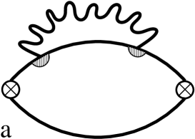
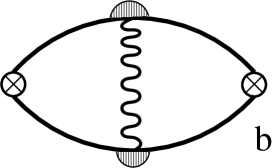
Figure 2: Diagrams representing various fluctuation contributions to the thermal conductivity. (a) density of states contribution. (b) Maki-Thompson contribution. The solid lines are impurity-averaged single-electron Green’s functions, wavy lines represent the fluctuation propagator and the shadowed areas are Cooperon vertex corrections. Crossed circles represent tunneling vertices.

The correction due to the density of states renormalization, Fig. 2(a), is the only one which is present even in absence of tunneling; therefore, for temperatures $T-T_{c}\gg g_{T}\delta$, we expect this term to give a significant contribution to the thermal conductivity. For lower temperatures, the bulk behaviour will be recovered.
The MT correction, represented in Fig. 2(b), can be evaluated using the same procedure as in the case of the DOS one. It is important to stress that the sign of linear response function is the same as for the DOS: in fact, the energies of electrons entering the diagram from opposite sides have opposite signs but the same happens to their velocities. In the case of electrical conductivity, the sign of linear response function is opposite. It is this difference that ultimately results in the cancellation of two identical contributions in the thermal conductivityNS02 .
Let us finally comment on the AL contribution, given by the diagrams in Fig. 3. It is well known, in the case of homogeneous metals, that such a correction to the thermal conductivity is not singular NS02 ; USH02 . We will show briefly that in the case of granular metals this correction vanishes nota2 in the static limit too, but not in the dynamical one, giving an important and characteristic contribution to the total correction.
In the following paragraphs, we present the evaluation of corrections to thermal conductivity due to different diagrams.

III.1 Density of states correction

The diagram for the DOS correction is given in Fig. 2(a) and the corresponding response function can be written as

$${\cal Q}^{\mathrm{(DOS)}}\left(\omega_{\nu}\right)=T^{2}t^{2}a^{2}\sum_{\left\langle i,j\right\rangle}\sum_{\Omega_{\mu}}\Lambda_{ij}\left(\Omega_{\mu}\right)\Sigma\left(\Omega_{\mu},\omega_{\nu}\right)\;,$$ (12)

where

$$\Sigma\left(\Omega_{\mu},\omega_{\nu}\right) = \sum_{\varepsilon_{n}}\lambda^{2}\left(\varepsilon_{n+\nu},\varepsilon_{-n-\nu+\mu}\right)\left(\varepsilon_{n}+\varepsilon_{n+\nu}\right)^{2}$$ (13)

$$\times I\left(\varepsilon_{n},\Omega_{\mu},\omega_{\nu}\right)\;,$$

and

$$I\left(\varepsilon_{n},\Omega_{\mu},\omega_{\nu}\right) = \int\left(dp\right)G^{2}_{0}\left({\bf p},\varepsilon_{n+\nu}\right)G_{0}\left({\bf p},\varepsilon_{-n-\nu+\mu}\right)$$ (14)

$$\times\int\left(dp^{\prime}\right)G_{0}\left({\bf p}^{\prime},\varepsilon_{n}\right).$$

We introduced the Cooperon vertex correction, $\lambda\left(\varepsilon_{1},\varepsilon_{2}\right)=1/\tau{\left|\varepsilon_{1}-\varepsilon_{2}\right|}$ in the zero-dimensional limit and without tunneling correctionsnota1 . The main contribution to singular behaviour comes from “classical” frequencies, $|\Omega_{\mu}|\ll T_{c}$: consequently, we will take the so-called static limit, $\Omega_{\mu}=0$, in the calculation of correction. This will be true also for the Maki-Thompson correction in the next paragraph. In the dirty limit, we can neglect all the energy scales in the electronic Green’s function in comparison with $1/\tau\gg T$, and the factor $I\left(\varepsilon_{n},0,\omega_{\nu}\right)$ turns out to be

$$I\left(\varepsilon_{n},0,\omega_{\nu}\right)=-2\left(\pi\nu_{F}\tau\right)^{2}\left[\theta\left(\varepsilon_{n}\varepsilon_{n+\nu}\right)-\theta\left(-\varepsilon_{n}\varepsilon_{n+\nu}\right)\right]\;.$$

Inserting the previous expression in Eq.(13), we are left with the sum over the electronic Matsubara frequencies. It is straightforward to check that the only contribution linear in $\omega_{\nu}$ is given by $\Sigma\left(0,\omega_{\nu}\right)=-\omega_{\nu}\pi\nu_{F}^{2}$. By means of Eq.(12), we obtain the general form for the DOS response function after the analytical continuation

$${\cal Q}^{\mathrm{(DoS)}}\left(-i\omega\right)=\left(-i\omega\right)\frac{8}{\pi}g_{T}Ta^{2}\sum_{\left\langle i,j\right\rangle}\Lambda_{ij}\left(0\right)\;,$$ (15)

where we also took into account the multiplicity of the DOS diagrams. The corresponding correction to heat conductivity is given by

$$\frac{\delta\kappa^{(DoS)}}{\kappa_{0}}=-\frac{3}{\pi^{2}}\frac{1}{g_{T}}\frac{g_{T}\delta}{T_{c}}\int_{BZ}(dK)\frac{1}{\epsilon+z\frac{g_{T}\delta}{T_{c}}\left(1-\gamma_{\bf K}\right)}.$$ (16)

We took the lattice Fourier transform and defined the reduced temperature $\epsilon=\ln(T/{T_{c}})\simeq{(T-T_{c})}/{T_{c}}$. $(dK)=[{a^{d}}/{(2\pi)^{d}}]d^{d}K$ is the dimensionless measure of the first Brillouin zone. Close to $T_{c}$, the integral takes its main contribution from the small momentum region and we recover the bulk DOS behaviour as

$$\delta\nu\propto\frac{1}{g_{T}}\left\{\begin{array}[]{cc}\sqrt{\epsilon},&d=3;\\ \ln\frac{1}{\epsilon},&d=2;\\ \frac{1}{\sqrt{\epsilon}},&d=1.\end{array}\right.$$ (20)

III.2 Maki-Thompson correction

The MT correction, [Fig. 2(b)], reads

$${\cal Q}^{\mathrm{(MT)}}\left(\omega_{\nu}\right)=a^{2}Tt^{2}\sum_{\left\langle i,j\right\rangle}\sum_{\Omega_{\mu}}\Lambda_{ij}\left(\Omega_{ij}\right)\Sigma\left(\Omega_{\mu},\omega_{\nu}\right)\;,$$ (21)

where

$$\Sigma\left(\Omega_{\mu},\omega_{\nu}\right) = T\sum_{\varepsilon_{n}}\lambda\left(\varepsilon_{n+\nu},\varepsilon_{-n-\nu+\mu}\right)\lambda\left(\varepsilon_{n},\varepsilon_{-n+\mu}\right)$$ (22)

$$\times\left(\varepsilon_{n}+\varepsilon_{n+\nu}\right)^{2}I\left(\varepsilon_{n},\Omega_{\mu},\omega_{\nu}\right)\;,$$

and

$$I\left(\varepsilon_{n},\Omega_{\mu},\omega_{\nu}\right) =\int\left(dp\right)G_{0}\left({\bf p},\varepsilon_{n+\nu}\right)G_{0}\left({\bf p},\varepsilon_{-n-\nu+\mu}\right)$$ (23)

$$\times\int\left(dp^{\prime}\right)G_{0}\left({\bf p}^{\prime},\varepsilon_{n}\right)G_{0}\left({\bf p}^{\prime},\varepsilon_{-n+\mu}\right).$$

Using the same procedure outlined above to calculate the DOS correction, we get

$$\frac{\delta\kappa^{(MT)}}{\kappa_{0}}=\frac{3}{\pi^{2}}\frac{1}{g_{T}}\frac{g_{T}\delta}{T_{c}}\int_{BZ}(dK)\frac{\gamma_{\bf K}}{\epsilon+z\frac{g_{T}\delta}{T_{c}}\left(1-\gamma_{\bf K}\right)}.$$ (24)

As expected, the MT correction has the same singular behaviour as the DOS but opposite sign. On the other hand, because such a correction involves the coherent tunneling of the fluctuating Cooper pair from one site to the nearest neighbor, it is proportional to the lattice structure factor $\gamma_{\bf K}$: due to this proportionality, in the regime $T-T_{c}\gg g_{T}\delta$, the correction vanishes because $\int_{BZ}(dK)\gamma_{\bf K}\equiv 0$. Let us stress again that this is not the case for the DOS correction, which in this regime behaves as $-(1/g)({E_{T}}/{T_{c}})(1/\epsilon)$.

III.3 Aslamazov-Larkin correction

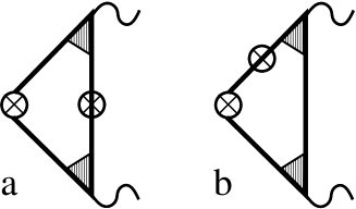
Figure 3: Diagrams of the blocks appearing in the Aslamazov-Larkin contribution to thermal conductivity. (b) has a double molteplicity, since the bare tunnel vertex can stay on both side of the block.

The AL diagrams can be built up by means of blocks in Fig. 3, by considering all their possible combinations in pairs. For a sake of simplicity, we will call the first block, Fig. 3(a), $B_{1}$, and the second one $B_{2}$. Finally, one has three different kind of diagrams: the first one, with two $B_{1}$-type blocks; the second one with two $B_{2}$-type blocks, and the latter, with both of them. Because of the double molteplicity of $B_{2}$-type block, one has a total of nine diagrams contributing to thermal conductivity. In the following, first we evaluate the analytical expression of $B_{1}$ and $B_{2}$ in the static approximation, then in the dynamical one, giving the expression of the total AL correction.
The general expression of response function for the AL diagrams reads

$${\cal Q}^{\mathrm{(AL)}}\left(\omega_{\nu}\right) =T^{2}a^{2}t^{4}\sum_{\begin{subarray}{c}\langle l,i\rangle\\ \langle j,m\rangle\end{subarray}}\sum_{\Omega_{\mu}}\Lambda_{ij}\left(\Omega_{\mu+\nu}\right)\Lambda_{ml}\left(\Omega_{\mu}\right)$$ (25)

$$\times B_{\mathrm{left}}\left(\omega_{\nu},\Omega_{\mu}\right)B_{\mathrm{right}}\left(\omega_{\nu},\Omega_{\mu}\right)\;,$$

where $B_{\mathrm{left}}$ and $B_{\mathrm{right}}$ can be either $B_{1}$ or $B_{2}$-type.
$B_{1}$ block reads

$$B_{1}\left(\omega_{\nu},\Omega_{\mu}\right) =\sum_{\varepsilon_{n}}\left(\varepsilon_{n}+\varepsilon_{n+\nu}\right)\lambda\left(\varepsilon_{n+\nu},\varepsilon_{\mu-n}\right)\lambda\left(\varepsilon_{n},\varepsilon_{\mu-n}\right)$$ (26)

$$\times\int(dp)G_{0}\left({\bf p},\varepsilon_{n+\nu}\right)G_{0}\left({\bf p},\varepsilon_{\mu-n}\right)$$

$$\times\int(dp^{\prime})G_{0}\left({\bf p}^{\prime},\varepsilon_{\mu-n}\right)G_{0}\left({\bf p}^{\prime},\varepsilon_{n}\right).$$

Taking the integrals over the Fermi surface, in the static approximation, we get

$$B_{1}\left(\omega_{\nu},0\right) = \left(2\pi\nu_{F}\tau\right)^{2}\sum_{\varepsilon_{n}}\theta\left(\varepsilon_{n+\nu}\varepsilon_{n}\right)\left(\varepsilon_{n}+\varepsilon_{n+\nu}\right)$$ (27)

$$\times\;\lambda\left(\varepsilon_{n+\nu},-\varepsilon_{n}\right)\lambda\left(\varepsilon_{n},-\varepsilon_{n}\right)$$

$$= \left(2\pi\nu_{F}\right)^{2}$$

$$\times\left[\sum_{\varepsilon_{n}<-\omega_{\nu}}+\sum_{\varepsilon_{n}>0}\right]\frac{\varepsilon_{n}+\varepsilon_{n+\nu}}{\left|\varepsilon_{n+\nu}+\varepsilon_{n}\right|}\frac{1}{\left|2\varepsilon_{n}\right|};$$

manipulating the sum, it is easy to see that

$$B_{1}\left(\omega_{\nu},0\right) = \left(2\pi\nu_{F}\right)^{2}\sum_{0<\varepsilon_{n}<\omega_{\nu}}\frac{1}{2\varepsilon_{n}}$$ (28)

$$= (2\pi\nu_{F})^{2}\left[\psi\left(\frac{\omega_{\nu}}{2\pi T}+\frac{1}{2}\right)-\psi\left(\frac{1}{2}\right)\right]$$

$$\approx \left(\frac{\pi\nu_{F}}{2}\right)^{2}\frac{\omega_{\nu}}{T}\;.$$

In the same way as sketched above, one can show, always in the static approximation, that the block $B_{2}$ vanishes identically. Then, all the diagrams containing $B_{2}$-type blocks do not give any contribution. Since the only AL diagram with two $B_{1}$-type block is proportional to the square of Eq. (28), it is quadratic in the external frequency $\omega$, and therefore vanishes identically in the limit $\omega\rightarrow 0$.
To evaluate the first non vanishing AL correction, one has to consider the dynamical contribution. In such a case, the $B_{2}$ block, for instance, reads

$$B_{2}\left(\omega_{\nu},\Omega_{\mu}\right) =\sum_{\varepsilon_{n}}\left(\varepsilon_{n}+\varepsilon_{n+\nu}\right)\lambda\left(\varepsilon_{n+\nu},\varepsilon_{\mu-n}\right)\lambda\left(\varepsilon_{n},\varepsilon_{\mu-n}\right)$$ (29)

$$\times\int(dp^{\prime})G_{0}\left({\bf p}^{\prime},\varepsilon_{\mu-n}\right)G_{0}\left({\bf p}^{\prime},\varepsilon_{n}\right)G_{0}\left({\bf p}^{\prime},\varepsilon_{n+\nu}\right)$$

$$\times\int(dp)G_{0}\left({\bf p},\varepsilon_{n+\nu}\right)\;.$$

In the evaluation of the block, because of the pole structure of fluctuation propagator, one can neglect the $\omega_{\nu}$ dependenceLV04 ; ISS03 , and keep just the one in $\Omega_{\mu}$. The calculation of the integrals and the sums in the latter equation is, in the dynamical approximation, a little bit more cumbersome. One has to take into account the different possible signs of $\Omega_{\mu}$ and $\varepsilon_{n}$. Finally, Eq. (29) reads

$$B_{2}\left(0,\Omega_{\mu}\right)=-2(\pi\nu_{F})^{2}\sum_{\varepsilon_{n}}\frac{2\varepsilon_{n}}{(2\varepsilon_{n}-\Omega_{\mu})^{2}}[\theta(\Omega_{\mu})(\theta(\varepsilon_{n}-\Omega_{\mu})$$ (30)

$$+\theta(-\varepsilon_{n}))+\theta(-\Omega_{\mu})(\theta(\Omega_{\mu}-\varepsilon_{n})+\theta(\varepsilon_{n}))]\;,$$

$\theta(x)$ being the step function.
By taking the lowest order in the bosonic frequency $\Omega_{\mu}$, one gets the result for the block

$$B_{2}\left(0,\Omega_{\mu}\right)=-\frac{1}{2}\left(\frac{\pi\nu_{F}}{2T}\right)^{2}\Omega_{\mu}\;.$$ (31)

In the same way, one can evaluate also $B_{1}$ with the result

$$B_{1}\left(0,\Omega_{\mu}\right)=-2B_{2}\left(0,\Omega_{\mu}\right)\;,$$ (32)

which is consistent with the homogeneous caseLV04 ; ISS03 . The sum over $\Omega_{\mu}$ in the response function can be performed by writing the sum as an integralLV04 , and exploiting the properties of the pair correlators.
Finally, the AL dynamical correction to thermal conductivity reads

$$\frac{\delta\kappa^{(AL)}}{\kappa_{0}}=\frac{9}{2\pi}\frac{1}{g_{T}}\left(\frac{g_{T}\delta}{T_{c}}\right)^{2}\int_{BZ}(dK)\frac{(1-\gamma_{\bf k})^{2}}{\epsilon+z\frac{g_{T}\delta}{T_{c}}\left(1-\gamma_{\bf K}\right)}\;.$$ (33)

The latter equation is the first non vanishing correction due to AL channel. Such a correction is always positive, and it depends, as in the MT, on the lattice structure factor $\gamma_{\bf K}$, but it does not vanishes in the regime $T-T_{c}\gg g_{T}\delta$. This is a good feature of the system, since far from $T_{c}$, the dynamical contribution plays an important role, and in this region, one has to compare it with DOS one, as discussed in the following section. Here, we just observe that since the corrections, Eqs. (16), (24) and (33), have different signs, nonmonotonic behaviour in the total correction is expected, depending on the ratio ${g_{T}\delta}/{T_{c}}$.

IV Discussion

As we have seen, the total superconducting fluctuation correction to the thermal conductivity close to critical temperature is given by the following expression

$$\frac{\delta\kappa}{\kappa_{0}}=\frac{3}{\pi^{2}}\frac{\delta}{T_{c}}\int_{BZ}(dK)\frac{\left(1-\gamma_{\bf K}\right)\left[\frac{3\pi}{2}\frac{g_{T}\delta}{T_{c}}\left(1-\gamma_{\bf K}\right)-1\right]}{\epsilon+z\frac{g_{T}\delta}{T_{c}}\left(1-\gamma_{\bf K}\right)}.$$ (34)

This correction has been obtained at all orders in the tunneling amplitude in the ladder approximation. Its behaviour is plotted in Fig. 4 as a function of the reduced temperature for the case of a two dimensional sample, and for different values of the ratio $g_{T}\delta/T_{c}$. We can recognize two different regimes of temperatures: far from $T_{c}$, $\epsilon\gg{g_{T}\delta}/{T_{c}}$, and close to $T_{c}$, $\epsilon\ll{g_{T}\delta}/{T_{c}}$. For a sake of simplicity, we will identify these two regimes as “high temperatures” and “low temperatures”, respectively.

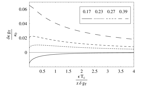
Figure 4: Total fluctuation correction to the thermal conductivity for different values of ${g_{T}\delta}/{T_{c}}$ for a two-dimensional system. A $1/\epsilon$ suppression is observed at high temperatures, with a sign depending on such ratio. At low temperatures, a finite correction, inversely proportional to the coordination number $z$, is reached at $\epsilon=0$. In a finite interval of values of $g_{T}\delta/T_{c}$, a nonmonotonic behaviour of the correction is observed, where the correction is positive and increasing with decreasing temperature, reaches a maximum and then goes to a smaller (possibly negative) value at the critical temperature.

• High temperature regime $\epsilon\gg{g_{T}\delta}/{T_{c}}$. In this region, the electrons do not tunnel efficiently between the grains and the system behaves almost as an ensemble of zero-dimensional systems. As a consequence, only the DOS and AL terms contribute significantly to the superconducting fluctuations; the correction to heat conductivity reads

  $$\frac{\delta\kappa}{\kappa_{0}} \approx \frac{3}{\pi^{2}}\frac{\delta}{T_{c}}\frac{1}{\epsilon}\left[\frac{3\pi}{2}\frac{g_{T}\delta}{T_{c}}\left(1+\frac{1}{z}\right)-1\right]\;.$$ (35)

  This expression shows a $1/\epsilon$ singularity and it can have either positive or negative sign, depending on the ratio $g_{T}\delta/T_{c}$; we call $\gamma_{1}$ the value of the above-mentioned ratio solution of Eq. (35). In the absence of renormalization due to tunnelling, the correction is negative and corresponds to the typical singularity of the quasi-zero-dimensional density of state. On the other hand, increasing the barrier transparency $g_{T}\delta$, the correction grows due to the presence of the direct channel, i.e., the AL term, which becomes more and more important, until the correction itself vanishes at $\gamma_{1}$, after which it becomes positive. A direct comparison with the behaviour of the electrical conductivityBEL00 shows that, already at this level, there is a positive violation of the Wiedemann-Franz law, being

  $$\frac{\delta L}{L_{0}} = \frac{\delta\kappa}{\kappa_{0}}-\frac{\delta\sigma}{\sigma_{0}}$$ (36)

  $$\approx \left[-\frac{3}{\pi^{2}}+\frac{9}{2\pi}\frac{g_{T}\delta}{T_{c}}\frac{z+1}{z}+\frac{7\zeta(3)}{\pi^{2}}\right]\frac{\delta}{T_{c}}\frac{1}{\epsilon}$$

• Low temperature regime $\epsilon\ll{g_{T}\delta}/{T_{c}}$. Here the tunneling is effective and there is a crossover to the typical behaviour of a homogeneous system, as $T\rightarrow T_{c}$, from the point of view of the fluctuating Cooper pairs. Physically, the bulk behaviour is recovered, and one gets a non divergent (though nonanalytic) correction even at $\epsilon=0$, where it equals

  $$\frac{\delta\kappa\left(\epsilon=0\right)}{\kappa_{0}}=\frac{3}{z\pi^{2}}\frac{1}{g_{T}}\left(\frac{3\pi}{2}\frac{g_{T}\delta}{T_{c}}-1\right)\;.$$ (37)

  The latter equation gives the saturation value in any dimension; it is also evident the $1/{g_{T}}$ order of the perturbation theory. Again, the value of the constant can be either negative or positive. The correction vanishes at a value $g_{T}\delta/T_{c}=\gamma_{2}$ which is independent on the dimensionality and larger than $\gamma_{1}$. In the interval $\gamma_{1}<g_{T}\delta/T_{c}<\gamma_{2}$, it has a non-monotonic behaviour, being positive and increasing for high temperatures and negative for low temperatures. Such a behaviour has been represented, for the case of $d=2$, in Fig.4. The deviation from the Wiedemann-Franz law in the low temperature region is much more evident than in the high temperature one, because of the pronounced singular behaviour of the electrical conductivity close to the critical temperatureBEL00 .

V Conclusions

We have calculated the superconducting fluctuation corrections to heat conductivity. In the region of temperatures $T-T_{c}\gg g_{T}\delta$, a strong singular correction is found, reported in Eq. (35), corresponding to the sum of the DOS renormalization and the AL contribution in a quasi-zero-dimensional system. Moving closer to the critical temperature, when $T-T_{c}\ll g_{T}\delta$, the divergent behaviour of the DOS term is cut off by the MT correction, which has opposite sign, while the AL term regularizes by itself to a finite value; this regularization signals the fact that the system undergoes a crossover to the homogeneous limit. A nondivergent behaviour is found at the critical temperature, in agreement with previous calculation in homogeneous superconductorsNS02 ; USH02 . The energy scale that separates the two regions, $g_{T}\delta$, can be recognized as the inverse tunneling time for a single electronBEAH01 . As a final remark, we want to note that the ratio $zg_{T}\delta/T_{c}$ appears as the coefficient of the ${\bf K}-$dependent term in the superconducting fluctuation propagator, Eq. (11): from the standard theory of the superconducting fluctuations, the coefficient of $K^{2}$ in the propagator is actually the superconducting coherence lengthLV04 ; we can therefore define an ”effective tunneling superconducting coherence length” as $\xi_{0}^{(T)}=a\sqrt{g_{T}\delta/T_{c}}$. From this definition, we can see that, if $\xi_{0}^{(T)}\ll a$, the grains are strictly zero-dimensional at high-temperature and the correction to the thermal conductivity is always negative, while if $\xi_{0}^{(T)}\gg a$, the direct channel of the superconducting correlations is strong enough to change sign to such correction.

We gratefully acknowledge illuminating discussions with A. A. Varlamov, I.V. Lerner and I.V. Yurkevich. This work was supported by IUF (FWJH), and Université franco-italienne (R. Ferone).

Appendix A Microscopic derivation of fluctuation propagator

Here we report a short description of the derivation of Eq.(11), evaluated in Ref. BEL00 , to remind the reader the main steps and the main assumptions of the calculation. We start from the expression of the partition function in the interaction representation

$${\cal Z} = {\rm Tr}\;{\rm exp}\left({-\int_{0}^{\beta}\hat{H}(\tau)d\tau}\right)$$ (38)

$$={\rm Tr}\;\Bigg{\{}{\rm exp}\left({-\int_{0}^{\beta}\hat{H}_{0}(\tau)d\tau}\right)$$

$$\times T_{\tau}\;{\rm exp}\left({-\int_{0}^{\beta}\left[\hat{H}_{P}(\tau)+\hat{H}_{T}\right]d\tau}\right)\Bigg{\}}\;.$$

We decouple the electronic fields in $\hat{H}_{P}$ by means of Hubbard-Stratonovich transformation, introducing the order parameter field $\Delta$; because of our assumption, $E_{T}\gg\Delta$, the grains can be considered strictly zero dimensional and we can neglect the spatial coordinate dependence in the field $\Delta_{i}$ in Eq. (38). We now expand over the field $\Delta_{i}$; the expansion is justified by our assumption to be close but above to the critical temperature where the mean field (BCS) value of order parameter is still zero; moreover, we have to expand the action to the second order in $t$, too; this expansion is justified in the region LY00 $t\ll 1/\tau\ll E_{T}$. We obtain two different contributions to the action: the first one is the typical action of superconducting fluctuations; the other one is the tunneling correction: $S_{\mathrm{eff}}=S_{\mathrm{eff}}^{0}+S_{\mathrm{eff}}^{t}$. The first term isLV04

$$S_{\mathrm{eff}}^{0}=-\frac{T}{V}\sum_{\Omega_{\mu}}\left|\Delta_{i}\left(\Omega_{\mu}\right)\right|^{2}$$ (39)

$$\times\Bigg{[}\frac{1}{\lambda}-4\pi\nu_{F}T{\rm\tau}\sum_{2\varepsilon_{n}>\Omega_{\mu}}\lambda\left(\varepsilon_{n},\varepsilon_{\mu-n}\right)\Bigg{]}\;.$$

$\Omega_{\mu}$ always appears as the combination of two fermionic Matsubara frequencies and it is therefore a bosonic one, as it should be. The sum over the fermionic frequencies in Eq. (39) is logarithmically divergent and must be cut off at Debye’s frequencyLV04 ; using the definition of superconducting critical temperature, one obtains

$$S_{\mathrm{eff}}^{0}=-\nu_{F}\frac{T}{V}\sum_{\Omega_{\mu}}\left|\Delta_{i}\left(\Omega_{\mu}\right)\right|^{2}$$

$$\times\Bigg{[}\ln\frac{T}{T_{c}}+\psi\left(\frac{1}{2}+\frac{\left|\Omega_{\mu}\right|}{4\pi T_{c}}\right)-\psi\left(\frac{1}{2}\right)\Bigg{]}\;,$$

where $\psi(x)$ is the digamma function, defined as the logarithmic derivative of gamma functionGR94 ; LV04 . Close to critical temperature, $T\simeq T_{c}$, as already mentioned, the main contribution to singular behaviour comes from ”classical” frequencies, $\left|\Omega_{\mu}\right|\ll T_{c}$. Then, we can expand the $\psi$ function in the small parameter ${\left|\Omega_{\mu}\right|}/{T_{c}}$:

$$S_{\mathrm{eff}}^{0}=-\nu_{F}\frac{T}{V}\sum_{{\bf K},\Omega_{\mu}}\left[\ln\frac{T}{T_{c}}+\frac{\pi\left|\Omega_{\mu}\right|}{8T_{c}}\right]\left|\Delta_{\bf K}\left(\Omega_{\mu}\right)\right|^{2}\;.$$ (40)

In the last expression, for later convenience, we considered the lattice Fourier transform: ${\bf K}$ belongs to the first Brillouin zone of reciprocal grain lattice. As it has been mentioned, the zero-dimensional character of the grain resides in the independence of the action on coordinates inside each grain.

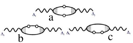
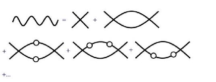
Figure 5: Top: The total tunneling correction to the fluctuation propagator self-energy is reported. The upper diagram is related to the possibility of tunneling of both electrons forming the fluctuating Cooper pair during the lifetime $\tau_{GL}$ of the Cooper pair itself. The other two diagrams consider the renormalization of the intragrain fluctuation propagator. Bottom: The ladder series for the fluctuation propagator in the presence of tunneling is reported. The crosses are BCS electron-electron interaction.

The tunneling-dependent part of the action is calculated starting from diagrams in Fig.5: they represent the first non-vanishing correction to fluctuation propagator due to tunneling. Their reexponentiation corresponds to the sum of the ladder series of tunneling and pairing interaction as reported in Fig.5. The calculation of diagram $a$, Fig.5(a), gives the contribution due to the possibility of tunneling of both electrons during the lifetime of the fluctuating Cooper pair, i.e. the Ginzburg-Landau time $\tau_{GL}=\pi/{8\left(T-T_{c}\right)}$; it is equal to

$$S_{\mathrm{eff}}^{t,(a)}=zg_{T}\sum_{{\bf K},\Omega_{\mu}}\gamma_{\bf K}\left|\Delta_{\bf K}\left(\Omega_{\mu}\right)\right|^{2}\;,$$ (41)

where, as mentioned, $z$ is the number of nearest neighbors.
Figures 5(b) and 5(c), give an identical contribution, which is related to the probability that a single electron, participating in the fluctuating Cooper pair, undergoes a double tunneling, back and forth, during the Ginzburg-Landau time. Such a contribution reads

$$S_{\mathrm{eff}}^{t,(b+c)}=-zg_{T}\sum_{{\bf K},\Omega_{\mu}}\left|\Delta_{\bf K}\left(\Omega_{\mu}\right)\right|^{2}.$$ (42)

The final result for fluctuation propagator at every order in tunneling in the ladder approximation is

$$\Lambda_{\bf K}\left(\Omega_{\mu}\right)=-\frac{1}{\nu_{F}}\frac{1}{\ln\frac{T}{T_{c}}+\frac{\pi\left|\Omega_{\mu}\right|}{8T_{c}}+z\frac{g_{T}\delta}{T_{c}}\left(1-\gamma_{\bf K}\right)}.$$ (43)

Finally, we notice that the classical limit ($\Omega_{\mu}=0$) for the fluctuation propagator Eq.(43) can be obtained from a straightforward generalization of the Ginzburg-Landau functional for granular metals

$${\cal F}\left[\Psi\right]=\sum_{\left\langle i,j\right\rangle}\int_{i}(d{\bf r})\int_{j}(d{\bf r}^{\prime})\Big{[}a\Psi_{i}^{*}\left({\bf r}\right)\Psi_{j}\left({\bf r}^{\prime}\right)\delta_{ij}\delta\left({\bf r}-{\bf r}^{\prime}\right)$$

$$+{\cal J}\left|\Psi_{i}\left({\bf r}\right)-\Psi_{j}\left({\bf r}^{\prime}\right)\right|^{2}\Big{]}$$ (44)

where the parameter $a$ is given by $(1/{4m\xi^{2}})\ln(T/{T_{c}})$, where $m$ is the electron mass, while the so-called Josephson parameter keep track of the tunneling effect: ${\cal J}=(1/{4m\xi^{2}})({zg_{T}\delta}/{T_{c}})$. See also Ref. DIG74, for the region of applicability of the theory reported above.

References

- (1) A.I. Larkin & A.A. Varlamov, Theory of Fluctuations in superconductors (Clarendon Press, Oxford, 2004).
- (2) A. Schmid, Phys. Kond. Mat. 5, 302 (1967).
- (3) C. Caroli & K. Maki, Phys. Rev. 164, 591 (1967).
- (4) I. Ussishkin, Phys. Rev. B 68, 024517 (2003).
- (5) E. Abrahams, M. Redi & J.W.F. Woo, Phys. Rev. B 1, 208 (1970).
- (6) D.R. Niven & R.A. Smith, Phys. Rev. B 66, 214505 (2002).
- (7) A. Gerber, A. Milner, G. Deutscher, M. Karpovsky, & A. Gladkikh, Phys. Rev. Lett. 78, 4277 (1997).
- (8) G. Balestrino, E. Milani & A.A. Varlamov, Physica C 210, 386 (1993).
- (9) F. Federici & A.A. Varlamov, Zh. Eksp. Teor. Fiz. 64, 397 (1996) [JETP Lett. 64, 497 (1996)]; Phys. Rev. B 55, 6070 (1997).
- (10) I.S. Beloborodov, K.B. Efetov & A.I. Larkin, Phys. Rev. B 61, 9145 (2000).
- (11) R.H. Parmenter, Phys. Rev. 154, 353 (1967).
- (12) G. Deutscher, Y. Imry & L. Gunther, Phys. Rev. B 10, 4598 (1974).
- (13) I.L. Kurland, I.L. Aleiner & B.L. Altshuler, Phys. Rev. B 62, 14886 (2000); Ya.M. Blanter, Phys. Rev. B 54, 12807 (1996); I.L Aleiner & L.I. Glazman Phys. Rev. B 57, 9608 (1998).
- (14) We assume that the tunneling contacts are not point-like. If they were (LY04, ; CML96, ), the tunneling conductance of the grains would be renormalized to by the backscattering: this fact is immediately understood saying that in this situation the average area of a tunneling contact is where is the Fermi wavelength and no more than one channel can be available for the transport. One is consequently forced to take into account higher-order diagrams in tunneling even in the Green’s function. On the other hand, if , higher-order diagrams will be smaller by a factor and in our approximation they can be safely neglected.
- (15) I.V. Lerner & I.V. Yurkevich, (unpublished).
- (16) J.C. Cuevas, A. Martin-Rodero & A. L. Yeyati, Phys. Rev. B 54, 7366 (1996).
- (17) C. Biagini, T. Caneva, V. Tognetti & A.A. Varlamov, Phys. Rev B 72, 041102 (2005).
- (18) I. Ussishkin, S.L. Sondhi & D.A. Huse, Phys. Rev. Lett. 89, 287001 (2002).
- (19) We thank Prof. A.A. Varlamov to have shown us this result.
- (20) The tunneling renormalization of the cooperon vertex correction is mandatory in the calculation of other thermodynamic or transport quantities, such as the correction to the superconducting critical temperatureBELV04 or the superconducting fluctuation corrections to the electrical conductivity in the absence of the magnetic fieldBEL00 , in order to avoid spurious divergences. In the case of the heat conductivity, such a renormalization gives only a small correction of the order of and can be safely neglected.
- (21) I.S. Beloborodov, K.B. Efetov, A. Altland & F.W.J. Hekking, Phys. Rev. B 63, 115109 (2001).
- (22) I.V. Yurkevich & I.V. Lerner, Phys. Rev. B 64, 054515 (2001).
- (23) I.S. Gradshtein & I.N. Ryzhik, Tables of Integrals, Series and Products (Alan Jeffrey Editor, Academic Press, San Diego, 1994).
- (24) I.S. Beloborodov, K.B. Efetov, A.V. Lopatin & V.M. Vinokur, Phys. Rev. B 71, 184501 (2005).