Nonequilibrium phenomena in multiple normal-superconducting tunnel heterostructures

Abstract

Using the nonequilibrium theory of superconductivity with the tunnel Hamiltonian, we consider a mesoscopic NISINISIN heterostructure, i.e., a structure consisting of five intermittent normal-metal (N) and superconducting (S) regions separated by insulating tunnel barriers (I). Applying the bias voltage between the outer normal electrodes one can drive the central N island very far from equilibrium. Depending on the resistance ratio of outer and inner tunnel junctions, one can realize either effective electron cooling in the central N island or create highly nonequilibrium energy distributions of electrons in both S and N islands. These distributions exhibit multiple peaks at a distance of integer multiples of the superconducting chemical potential. In the latter case the superconducting gap in the S islands is strongly suppressed as compared to its equilibrium value.

I Introduction

Mesoscopic electronic applications typically rely on phenomena which show best when the electrons in small wires are cooled to very low temperatures, ideally to the range of 10 mK. In this regime the crystal lattice is very weakly coupled to the electron system, and electron cooling via the lattice becomes difficult. An alternative approach is then to directly cool the electrons. This can be achieved by placing superconducting (S) contacts via insulating (I) barriers to the normal-metal (N) or superconducting (S^′) wire whose electrons are to be cooled nahum94 ; leivo96 ; GolubevVasenko . By applying a voltage over such SINIS/SIS^′IS coolers, it has been shown that one can cool electrons well below 100 mK with these structuresPekola2 , even when the lattice remains at a few hundred mK, or to enhance the superconductivity in the middle S^′ island SCenhancement1 ; SCenhancement2 ; HeslingaKlapwijk . Optimally, such cooling should take the electron temperature to a few mK, a limit which is hardly reached in mesoscopic systems via other known means.

With this type of nonequilibrium cooling, the concept of the electron temperature is not always well defined Pekola2 , but one has to rather describe the full electron energy distribution function Pothier ; Giazotto . In this case cooling corresponds to the sharpening of this distribution function, essentially removing the high-energy excitations.

One of the features limiting the performance of such SINIS coolers is the fact that the poor heat conductivity of the superconductors makes them inefficient reservoirs Pekola1 . An additional pair of normal-metal electrodes attached to superconducting electrodes of a SINIS cooler can improve the relaxation and enhance the cooling characteristics of the device GolubevVasenko . In this paper, we consider the effects of extra N electrodes of this type attached to a generic SINIS structure. The superconducting pieces are now assumed small enough so that they can be driven out of equilibrium by applying a bias voltage between the two normal electrodes. It is this arrangement of a NISIN^′ISIN multiple heterostructure which is the subject of the present study. Its novel feature as compared to the traditional SINIS structure with bulk S electrodes is that nonequilibrium is now induced in all inner islands of the structure, which, in turn, strongly enhances nonequilibrium effects both in the central N and in the adjacent S islands. The resulting distributions in each island can be inspected by transverse probe tunnel junctionsPothier ; Pekola2 .

The microscopic nonequilibrium theory of double-barrier SINIS junctions is based on time-dependent Keldysh Green function formalism (see Ref. Brinkman, and references therein). In the present paper we extend the theory such that nonequilibrium distributions in superconducting islands are also allowed. The major modification is that the chemical potentials of the two superconducting islands cannot be chosen zero simultaneously since these islands have different potentials determined by the bias voltage. This is equivalent to a time dependence of the order parameters imposed by different time-dependent order-parameter phases. We restrict ourselves to a tunneling Hamiltonian approximation which effectively makes the problem spatially independent within each superconducting or normal island.

II Model

The system we study is shown in Fig. 1. In nonequilibrium, each of the islands has a separate energy distribution and, according to our model based on the tunnel Hamiltonian, they are independent of both coordinates and directions of the momenta. This implies that each region is in a diffusive regime when the momentum direction dependence is averaged out within the first approximation in $\ell/L$ where $\ell$ is the impurity mean free path and $L$ is the length of the contacting region. In addition, one has to assume that the intrinsic normal-state resistance $r$ of each island is much smaller than any of the tunnel resistances $R$ to satisfy the condition that the potential variation inside each region is smaller than its drop across the tunnel barrier.

Figure 1: NISINISIN structure: The central normal island (N) is placed between two superconducting islands (S) which are connected to two outer N electrodes serving as external leads. Each connection is realized through a tunnel contact with a resistance $R_{ik}$.

A characteristic rate for tunneling from region 2 into region 1 to be defined later is $\eta_{12}=\left[4\nu_{1}e^{2}\Omega_{1}R\right]^{-1}$, where $\nu_{1}$ is the normal-state density of states (DOS) at the Fermi level in region 1 and $\Omega_{1}$ is the volume of conductor 1. Competing with the inelastic relaxation, this rate determines whether the injection of new quasiparticles into the system is fast enough to drive the system out of equilibrium. The inelastic processes which uphold the thermal Fermi distribution can be neglected if $\eta\gg 1/\tau_{\rm inel}$ which is equivalent to

$$\nu e^{2}\Omega R/\tau_{\rm inel}\sim\left(L\ell/\ell^{2}_{\rm inel}\right)\Gamma\ll 1$$ (1)

where $\Gamma=(N_{m}R/R_{Q})(\bar{A}/A)$. Here $\bar{A}$ stands for the average cross-section area of the conductor, $L$ is its length such that $\Omega=\bar{A}L$, $A$ is the area of the junction, $\ell_{\rm inel}=\sqrt{D\tau_{\rm inel}}$, and $D=v_{F}\ell/3$ is the diffusion coefficient. We also introduce the quantum resistance $R_{Q}=\pi\hbar/2e^{2}$, and the number of conducting modes $N_{m}\sim p_{F}^{2}A/\hbar^{2}$ in the area of the junction.

In our work, we assume that the electron energy distribution within each island is homogeneous, which also implies a homogeneous potential and a constant effective temperature. Analysis of kinetic equations shows that this is achieved if $r\ll R$ or

$$\sigma\bar{A}/L\sim\nu De^{2}\bar{A}/L\gg 1/R$$

which gives

$$DL^{-2}\gg(\nu e^{2}R\Omega)^{-1}\sim\eta\ .$$

This puts a restriction $L\ll\ell\Gamma$. The limit $\ell\ll L$ holds if $\Gamma\gg 1$. Our model is thus applicable provided $1\ll L/\ell\ll\Gamma$. Condition (1) of small inelastic interaction reads $\ell_{\rm inel}^{2}\gg\Gamma L\ell$.

III Formalism

III.1 Transport equation

We use the standard Keldysh Green function formalism, see for example Ref. KopninBook, . We denote the Nambu-space matrix operator

$$\hat{G}^{-1}=\hat{\tau}_{3}\frac{\partial}{\partial\tau}-\frac{\nabla^{2}}{2m}-\mu+\hat{H}\,,\;\hat{H}=\left(\begin{array}[]{cc}0&-\Delta\\ \Delta^{*}&0\end{array}\right).$$

It acts on matrix Green functions

$$\hat{G}=\left(\begin{array}[]{cc}G&F\\ -F^{\dagger}&\bar{G}\end{array}\right)\ ,$$

where $\hat{G}$ stands for either retarded (advanced), $\hat{G}^{R(A)}$, or Keldysh, $\hat{G}^{K}$, Green function. For tunnelling between two superconductors (or normal metals) 1 and 2, the self energy in region 1 is $\hat{\Sigma}_{T}(1)=i\eta_{12}\hat{g}(2)$ provided the semi-classical Green functions

$$\hat{g}=\int\frac{d\xi_{p}}{\pi i}\hat{G}\left({\bf p}+{\bf k}/2,{\bf p}-{\bf k}/2\right),$$

integrated over the energy $\xi_{p}=p^{2}/2m-E_{F}$, are independent of the directions of momentum ${\bf p}$. The tunneling rate is defined as

$$\eta_{12}=\pi\nu_{2}\Omega_{1}^{-1}\left<|T_{{\bf p},{\bf q}}|^{2}\right>=\left[4\nu_{1}e^{2}\Omega_{1}R_{12}\right]^{-1}\ .$$ (2)

Here $T_{{\bf p},{\bf q}}$ is the tunnel matrix element and $R_{12}$ is the tunnel resistance of the contact between regions 1 and 2. Note that the self-energy in region 2 is $\hat{\Sigma}_{T}(2)=i\eta_{21}\hat{g}(1)$ where $\eta_{21}=\pi\nu_{1}\Omega_{2}^{-1}\left<|T_{{\bf p},{\bf q}}|^{2}\right>=\left[4\nu_{2}e^{2}\Omega_{2}R_{12}\right]^{-1}$. If region 1 has tunnel contacts to two other regions 2 and 3, the self energy is a sum

$$\hat{\Sigma}_{T}(1)=i\eta_{12}\hat{g}(2)+i\eta_{13}\hat{g}(3)$$

where $\eta_{12}=\left[4\nu_{1}e^{2}\Omega_{1}R_{12}\right]^{-1}$ and $\eta_{13}=\left[4\nu_{1}e^{2}\Omega_{1}R_{13}\right]^{-1}$.

Including the tunnelling self-energy into the total self-energy that contains both elastic and inelastic processes we can write equations for the retarded, advanced, and Keldysh Green functions:

$$\left(\hat{G}^{-1}-\hat{\Sigma}^{R(A)}\right)\circ\hat{G}^{R(A)} = \hat{1}\delta(x_{1}-x_{2})\ ,$$

$$\left(\hat{G}^{-1}-\hat{\Sigma}^{R}\right)\circ\hat{G}^{K}-\hat{\Sigma}^{K}\circ\hat{G}^{A} = 0\ .$$

The product $\hat{\Sigma}^{K}\circ\hat{G}^{A}$ is a convolution over frequencies and momenta of the type

$$\hat{\Sigma}^{K}\circ\hat{G}^{A}=\int\hat{\Sigma}^{K}_{\epsilon_{1},\epsilon}\hat{G}^{A}_{\epsilon,\epsilon_{2}}\,\frac{d\epsilon}{2\pi}\ .$$

Applying the inverse operator to $\hat{G}^{R(A)}$ and $\hat{G}^{K}$ from the right and subtracting the obtained equations from the equations above we find the transport-like equations

$${\bf v}_{F}{\bf k}\hat{G}^{K}_{\epsilon_{1},\epsilon_{2}}-\epsilon_{1}\hat{\tau}_{3}\hat{G}^{K}_{\epsilon_{1},\epsilon_{2}}+\hat{G}^{K}_{\epsilon_{1},\epsilon_{2}}\epsilon_{2}\hat{\tau}_{3}$$

$$+\hat{H}\circ\hat{G}^{K}-\hat{G}^{K}\circ\hat{H} = \hat{\cal I}^{K}_{\epsilon_{1},\epsilon_{2}}\ ,$$ (3)

$${\bf v}_{F}{\bf k}\hat{G}^{R(A)}_{\epsilon_{1},\epsilon_{2}}-\epsilon_{1}\hat{\tau}_{3}\hat{G}^{R(A)}_{\epsilon_{1},\epsilon_{2}}+\hat{G}^{R(A)}_{\epsilon_{1},\epsilon_{2}}\epsilon_{2}\hat{\tau}_{3}$$

$$+\hat{H}\circ\hat{G}^{R(A)}-\hat{G}^{R(A)}\circ\hat{H} = \hat{\cal I}^{R(A)}_{\epsilon_{1},\epsilon_{2}}\ ,$$ (4)

where the collision integrals in each region are

$$\hat{\cal I}^{K}_{\epsilon_{1},\epsilon_{2}} = \hat{\Sigma}^{R}\circ\hat{G}^{K}-\hat{G}^{K}\circ\hat{\Sigma}^{A}-\hat{G}^{R}\circ\hat{\Sigma}^{K}+\hat{\Sigma}^{K}\circ\hat{G}^{A}\ ,$$

$$\hat{\cal I}^{R(A)}_{\epsilon_{1},\epsilon_{2}} = \hat{\Sigma}^{R(A)}\circ\hat{G}^{R(A)}-\hat{G}^{R(A)}\circ\hat{\Sigma}^{R(A)}\ .$$

We also define

$$\hat{I}^{K}_{\epsilon_{1},\epsilon_{2}}\equiv\left(\begin{array}[]{cc}I_{1}&I_{2}\\ -I_{2}^{\dagger}&\bar{I}_{1}\end{array}\right)=\int\frac{d\xi_{p}}{\pi i}\hat{\cal I}^{K}_{\epsilon_{1},\epsilon_{2}}\ .$$

Finally, the tunnel collision integral for region 1 in contact with region 2 takes the form

$$\hat{I}^{K}_{T}(1) = i\eta_{12}\left[\hat{g}^{R}(2)\circ\hat{g}^{K}(1)-\hat{g}^{R}(1)\circ\hat{g}^{K}(2)\right.$$ (5)

$$\left.+\hat{g}^{K}(2)\circ\hat{g}^{A}(1)-\hat{g}^{K}(1)\circ\hat{g}^{A}(2)\right]\ .$$

If the distribution function is time independent, the Keldysh Green function has the form

$$\hat{g}^{K}_{\epsilon_{1},\epsilon_{2}}=\hat{g}^{R}_{\epsilon_{1},\epsilon_{2}}\left(f_{1,\epsilon_{2}}+\hat{\tau}_{3}f_{2,\epsilon_{2}}\right)-\left(f_{1,\epsilon_{1}}+\hat{\tau}_{3}f_{2,\epsilon_{1}}\right)\hat{g}^{A}_{\epsilon_{1},\epsilon_{2}},$$ (6)

where the odd- and even-in-$\epsilon$ distribution functions $f_{1}$ and $f_{2}$ are defined such that

$$f_{1,\epsilon}=-n(\epsilon)+n(-\epsilon)\,,\;f_{2,\epsilon}=1-n(-\epsilon)-n(\epsilon)\ .$$

The actual quasiparticle energy distribution function $n$ satisfies $f_{1,\epsilon}+f_{2,\epsilon}=1-2n(\epsilon)$.

For spatially uniform distributions the kinetic equations in each conducting region is obtained after averaging Eqs. (3), (4) over the momentum directions. The elastic collision integrals average out, and the kinetic equations for diagonal in $\epsilon$ components become

$${\rm Tr}\left(\hat{M}_{\epsilon,\epsilon}\right) = {\rm Tr}\left[\hat{I}^{K}_{\epsilon,\epsilon}-\left(\hat{I}^{R}_{\epsilon,\epsilon}-\hat{I}^{A}_{\epsilon,\epsilon}\right)f_{1,\epsilon}\right]\ ,$$ (7)

$${\rm Tr}\left(\hat{\tau}_{3}\hat{M}_{\epsilon,\epsilon}\right) = {\rm Tr}\left(\hat{\tau}_{3}\left[\hat{I}^{K}-\left(\hat{I}^{R}_{\epsilon,\epsilon}-\hat{I}^{A}_{\epsilon,\epsilon}\right)f_{1,\epsilon}\right]\right)\ .$$ (8)

The collision integrals here include only tunnel and inelastic contributions $\hat{I}=\hat{I}_{T}+\hat{I}_{\rm inel}$, where inelastic processes include electron-phonon and electron-electron interactions, $\hat{I}_{\rm inel}=\hat{I}_{\rm e-ph}+\hat{I}_{\rm e-e}$. The matrix $\hat{M}$ is

$$\hat{M} = \left(\hat{H}\circ\hat{g}^{K}-\hat{g}^{K}\circ\hat{H}\right)$$

$$-\left(\hat{H}\circ\hat{g}^{R}-\hat{g}^{R}\circ\hat{H}\right)f_{1}+f_{1}\left(\hat{H}\circ\hat{g}^{A}-\hat{g}^{A}\circ\hat{H}\right)\ .$$

III.2 Charge and energy tunnel currents

After taking the trace and integrating over energy and momentum, Eq. (3) in region 1 yields

$$-\frac{\partial}{\partial t}\left(\nu_{1}\int\frac{d\epsilon}{2}\int\frac{d\xi_{1}}{\pi i}\frac{d\Omega_{\bf p}}{4\pi}{\rm Tr}\,\hat{G}^{K}\right)$$

$$=-i\nu_{1}\int\frac{d\epsilon}{2}\frac{d\Omega_{\bf p}}{4\pi}{\rm Tr}\,\left[\hat{\tau}_{3}\hat{I}^{K}(1)\right]\ ,$$

which is the conservation of charge $Q(1)=eN(1)\Omega_{1}$ in the volume $\Omega_{1}$ of region 1:

$$\frac{\partial Q(1)}{\partial t}=I(1)\ .$$ (9)

Here $N(1)$ is the particle density in region 1. The current that flows into region 1 is

$$I(1)=-ie\nu_{F1}\Omega_{1}\int\frac{d\epsilon}{4}\frac{d\Omega_{\bf p}}{4\pi}{\rm Tr}\,\left[\hat{\tau}_{3}\hat{I}^{K}_{T}(1)\right]\ .$$ (10)

The inelastic collision integral drops out because it conserves the particle number.

Multiplying Eq. (3) by $\epsilon$ and taking the trace of it one can obtain the balance of the energy ${\cal E}=\Omega E$ in the form

$$\frac{\partial{\cal E}(1)}{\partial t}=I_{\cal E}(1).$$

Here the energy density is

$$E=-\int\epsilon{\rm Tr}\,\left(\hat{\tau}_{3}\hat{G}^{K}_{\epsilon_{+},\epsilon_{-}}\right)\frac{d\epsilon}{4\pi i}\frac{d^{3}p}{(2\pi)^{3}}+\frac{|\Delta|^{2}}{|g|}-Ne\varphi$$

and the energy current into region 1 is

$$I_{\cal E}(1)=-i\nu_{1}\Omega_{1}\int\frac{d\epsilon}{4}\frac{d\Omega_{\bf p}}{4\pi}{\rm Tr}\,\left[\left(\epsilon-e\varphi_{1}\hat{\tau}_{3}\right)\hat{I}^{K}(1)\right]\ .$$ (11)

The collision integral in Eq. (11) contains both tunnel and electron-phonon contributions, $I^{K}(1)=I^{K}_{\rm e-ph}(1)+I^{K}_{T}(1)$. The electron-electron interactions drop out because of the energy conservation. The energy flow into region 1 can be separated into two parts. One part containing $I^{K}_{\rm e-ph}$ is the energy exchange with the heat bath (phonons). The other part contains the tunnel contribution $I^{K}_{T}(1)$ and is the energy current into region 1 through the tunnel contact.

IV Kinetic equations in hybrid structures

IV.1 Nonzero superconducting chemical potential

If a hybrid structure containing more than one superconducting island is voltage biased, at least one of the superconductors will have a nonzero chemical potential with a time dependent phase of the order parameter. If the external voltage is constant and the resulting state is stationary, the phase is linear in time, $\chi=2\mu_{S}t$, while the magnitude of the order parameter is time independent. Consider two sets of regular Green functions. One set of functions $\hat{g}^{R(A)}$ is taken in the basis where the order parameter phase varies in time. The other set belongs to the same order parameter magnitude but has a phase constant in time (zero for simplicity). However, the energies of the Green-functions $g^{R(A)}$, $\bar{g}^{R(A)}$, $f^{R(A)}$, and $f^{\dagger R(A)}$ are shifted by different amounts proportional to the chemical potential in the previous representation. The relations between these two sets, the Green functions $g^{R(A)}_{\epsilon,\epsilon^{\prime}}$ and $f^{R(A)}_{\epsilon,\epsilon^{\prime}}$ and the steady-state functions with shifted energies, can be established from the Eilenberger equations. Since $\Delta=|\Delta|e^{+i2\mu_{S}t}$, i.e.,

$$\Delta_{\omega}=|\Delta|2\pi\delta(\omega+2\mu_{S})\,,\;\Delta^{*}_{\omega}=|\Delta|2\pi\delta(\omega-2\mu_{S})\ ,$$

one observes that Eqs. (4) are satisfied by

$$g^{R(A)}_{\epsilon,\epsilon^{\prime}}=g^{R(A)}_{\epsilon+\mu_{S}}2\pi\delta(\epsilon-\epsilon^{\prime})\,,\;\bar{g}^{R(A)}_{\epsilon,\epsilon^{\prime}}=\bar{g}^{R(A)}_{\epsilon-\mu_{S}}2\pi\delta(\epsilon-\epsilon^{\prime})$$ (12)

and

$$f^{\dagger R(A)}_{\epsilon,\epsilon^{\prime}} = f^{\dagger R(A)}_{\epsilon-\mu_{S}}2\pi\delta(\epsilon-\epsilon^{\prime}-2\mu_{S})\ ,$$

$$f^{R(A)}_{\epsilon,\epsilon^{\prime}} = f^{R(A)}_{\epsilon+\mu_{S}}2\pi\delta(\epsilon-\epsilon^{\prime}+2\mu_{S})\ .$$ (13)

The functions $g^{R(A)}_{\epsilon}=-\bar{g}^{R(A)}_{\epsilon}$ and $f^{R(A)}_{\epsilon}=f^{\dagger R(A)}_{\epsilon}$ satisfy the steady-state Eilenberger equation

$$-2\epsilon f^{R(A)}_{\epsilon}+2|\Delta|g^{R(A)}_{\epsilon}=I_{2,\epsilon}^{R(A)}$$ (14)

supplemented with the normalization

$$\left[g^{R(A)}_{\epsilon}\right]^{2}-\left[f^{R(A)}_{\epsilon}\right]^{2}=1\ .$$ (15)

Therefore, we find from Eq. (6) for a nonzero chemical potential

$$g^{K}_{\epsilon,\epsilon^{\prime}} = \left[g^{R}_{\epsilon+\mu_{s}}-g^{A}_{\epsilon+\mu_{s}}\right]\left(f_{1,\epsilon}+f_{2,\epsilon}\right)2\pi\delta(\epsilon-\epsilon^{\prime})\ ,\quad$$ (16)

$$-\bar{g}^{K}_{\epsilon,\epsilon^{\prime}} = \left[g^{R}_{\epsilon-\mu_{s}}-g^{A}_{\epsilon-\mu_{s}}\right]\left(f_{1,\epsilon}-f_{2,\epsilon}\right)2\pi\delta(\epsilon-\epsilon^{\prime})\ .\quad$$ (17)

The off-diagonal Keldysh Green function in Eq. (6) becomes

$$f^{K}_{\epsilon,\epsilon-\omega} = \left[f^{R}_{\epsilon+\mu_{S}}(f_{1,\epsilon+2\mu_{S}}-f_{2,\epsilon+2\mu_{S}})\right.$$ (18)

$$\left.-(f_{1,\epsilon}+f_{2,\epsilon})f^{A}_{\epsilon+\mu_{S}}\right]\,2\pi\delta(\omega+2\mu_{s})\ .$$

IV.2 Tunnel collision integrals

Assume that region 1 is a superconductor and region 2 is a normal metal. With Eqs. (12), (16), and (17), the matrix elements of the tunnel collision integral Eq. (5) in the superconducting region $S$ give

$${\rm Tr}\left[\hat{I}^{K}_{T}(S)\right] = 4i\eta_{SN}\left\{\left[g_{\epsilon+\mu_{S}}(S)+g_{\epsilon-\mu_{S}}(S)\right]\left[f_{1,\epsilon}(S)-f_{1,\epsilon}(N)\right]+\left[g_{\epsilon+\mu_{S}}(S)-g_{\epsilon-\mu_{S}}(S)\right]\left[f_{2,\epsilon}(S)-f_{2,\epsilon}(N)\right]\right\},\qquad$$ (19)

$${\rm Tr}\left[\hat{\tau}_{3}\hat{I}^{K}_{T}(S)\right] = 4i\eta_{SN}\left\{\left[g_{\epsilon+\mu_{S}}(S)-g_{\epsilon-\mu_{S}}(S)\right]\left[f_{1,\epsilon}(S)-f_{1,\epsilon}(N)\right]+\left[g_{\epsilon+\mu_{S}}(S)+g_{\epsilon-\mu_{S}}(S)\right]\left[f_{2,\epsilon}(S)-f_{2,\epsilon}(N)\right]\right\}.\qquad$$ (20)

Components of the retarded and advanced tunnel collision integrals $\hat{I}^{R(A)}$ are

$$I^{R(A)}_{2}(S)=\pm i\eta_{SN}f^{R(A)}(S)\,,\;-I^{\dagger R(A)}_{2}(S)=\pm i\eta_{SN}f^{\dagger R(A)}(S)\,,\;I^{R(A)}_{1}(S)=\bar{I}^{R(A)}_{1}(S)=0\ .$$

Both Keldysh and R(A) tunnel collision integrals in the normal region N are coupled to those in the region S by $\eta_{SN}I(N)=-\eta_{NS}I(S)$.

Using Eqs. (13) and (18), we find

$${\rm Tr}\left(\hat{M}_{\epsilon,\epsilon}\right) = 2|\Delta|F_{\epsilon+\mu_{S}}\left(f_{1,\epsilon}-f_{1,\epsilon+2\mu_{S}}+f_{2,\epsilon}+f_{2,\epsilon+2\mu_{S}}\right)-2|\Delta|F^{R}_{\epsilon-\mu_{S}}\left(f_{1,\epsilon-2\mu_{S}}-f_{1,\epsilon}+f_{2,\epsilon}+f_{2,\epsilon-2\mu_{S}}\right),\quad$$ (21)

$${\rm Tr}\left(\hat{\tau}_{3}\hat{M}_{\epsilon,\epsilon}\right) = 2|\Delta|F_{\epsilon+\mu_{S}}\left(f_{1,\epsilon}-f_{1,\epsilon+2\mu_{S}}+f_{2,\epsilon}+f_{2,\epsilon+2\mu_{S}}\right)+2|\Delta|F_{\epsilon-\mu_{S}}\left(f_{1,\epsilon-2\mu_{S}}-f_{1,\epsilon}+f_{2,\epsilon}+f_{2,\epsilon-2\mu_{S}}\right).\quad$$ (22)

After inserting Eqs. (19), (20) and (21), (22) into Eqs. (7) and (8) they yield the final kinetic equations to be solved for the distribution functions.

In the equations above, we introduce $g_{\epsilon}=\left(g^{R}_{\epsilon}-g^{A}_{\epsilon}\right)/2\equiv{\rm Re}\,g^{R}_{\epsilon}$ and also $F_{\epsilon}=\left(f^{R}_{\epsilon}+f^{A}_{\epsilon}\right)/2\equiv i\,{\rm Im}\,f^{R}_{\epsilon}$. The functions $g_{\epsilon}$ and $F_{\epsilon}$ are even in $\epsilon$. With the account of tunnel and electron-phonon interactions, they can be found from the steady-state Eilenberger equations (14), (15). These equations can be more easily solved when the inelastic interaction is small. If region 2 is normal, one finds

$$g^{R(A)}_{\epsilon} = \pm\frac{\epsilon\pm i\gamma}{\sqrt{\left(\epsilon\pm i\gamma\right)^{2}-|\Delta|^{2}}}\,,$$ (23)

$$f^{R(A)}_{\epsilon} = \pm\frac{|\Delta|}{\sqrt{\left(\epsilon\pm i\gamma\right)^{2}-|\Delta|^{2}}}\ ,$$ (24)

where $\gamma=\eta_{SN}$.

For a N₁IS₁INIS₂IN₂ structure, each conductor S₁, N, or S₂ has tunnel contacts with two other conductors, thus the tunnel integrals are sums of the contributions from two regions. For example, if the inelastic interaction is small, the depairing rate in Eqs. (23) and (24) is $\gamma(S_{i})=\eta_{S_{i}N}+\eta_{S_{i}N_{i}}$.

IV.3 Current conservation

For a NS junction, the tunnel current Eq. (10) into the superconductor S from a normal region N or N_1,2 is

$$I(N\rightarrow S) = \frac{1}{4eR_{SN}}\int_{-\infty}^{\infty}d\epsilon\,g_{\epsilon}(S)\left[f_{1,\epsilon-\mu_{S}}(S)-f_{1,\epsilon+\mu_{S}}(S)-f_{1,\epsilon-\mu_{S}}(N)+f_{1,\epsilon+\mu_{S}}(N)\right.$$ (25)

$$+\left.f_{2,\epsilon-\mu_{S}}(S)+f_{2,\epsilon+\mu_{S}}(S)-f_{2,\epsilon-\mu_{S}}(N)-f_{2,\epsilon+\mu_{S}}(N)\right]\ .$$

Electric currents through both junctions are balanced when $I(N\rightarrow S_{i})+I(N_{i}\rightarrow S_{i})=0$.

The energy current flowing into the superconducting island through each junction has the form

$$I_{\cal E}(N\rightarrow S) = \frac{1}{4e^{2}R_{NS}}\int_{-\infty}^{\infty}d\epsilon\,\epsilon\,g_{\epsilon}(S)\left(\left[f_{1,\epsilon-\mu_{S}}(S)+f_{1,\epsilon+\mu_{S}}(S)-f_{1,\epsilon-\mu_{S}}(N)-f_{1,\epsilon+\mu_{S}}(N)\right]\right.$$ (26)

$$+\left.\left[f_{2,\epsilon-\mu_{S}}(S)-f_{2,\epsilon+\mu_{S}}(S)-f_{2,\epsilon-\mu_{S}}(N)+f_{2,\epsilon+\mu_{S}}(N)\right]\right)-I(N\rightarrow S)[\mu_{S}/e+\varphi_{S}]\ .$$

The energy conservation follows from the kinetic equations and is therefore an abundant condition. However, in the quasi-equilibrium limit, when the electron-electron interaction in each island dominates over the tunnel injection, the distribution functions are nearly thermal with certain temperatures specific for each region. In this case, the kinetic equations do not need to be solved explicitly, but the temperatures are found by requiring the conservation of the energy current.

The energy current $I_{\cal E}(S\rightarrow N)$ flowing into the central normal island through each junction is obtained from Eq. (26) by changing the sign and replacing $\varphi_{S}$ with $\varphi_{N}$ so that the difference between the energy currents from N to S calculated in two opposite directions is $I_{\cal E}(N\rightarrow S)+I_{\cal E}(S\rightarrow N)=I(N\rightarrow S)V_{NS},$ where $V_{NS}=\varphi_{N}-\varphi_{S}$ is the voltage across the junction. This difference of energy currents is compensated by the work produced by the voltage source and does not lead to the change in the energy of the superconductor. When the energy currents into a superconducting island are balanced, the terms with $\mu_{S}/e+\varphi_{S}$ cancel due to the electric current conservation. In the normal island, however, only the terms with $\varphi_{N}$ drop out since the chemical potentials $\mu_{S}$ on both sides of the island are different.

IV.4 Self-consistency equation and charge neutrality

The magnitude of the order parameter is found from Eq. (18). It is a real quantity, therefore,

$$\frac{|\Delta|}{\lambda}=\int_{-E_{c}}^{E_{c}}\left({\rm Re}\,f^{R}_{\epsilon}\right)\left[f_{1,\epsilon+\mu_{S}}+f_{1,\epsilon-\mu_{S}}\right.$$

$$\left.-f_{2,\epsilon+\mu_{S}}+f_{2,\epsilon-\mu_{S}}\right]\,\frac{d\epsilon}{4}$$ (27)

where $E_{c}$ is the BCS cut-off energy. The self-consistency of the order parameter requires vanishing of its imaginary part:

$$\int_{-\infty}^{\infty}F_{\epsilon}\left(f_{1,\epsilon+\mu_{S}}-f_{1,\epsilon-\mu_{S}}-f_{2,\epsilon+\mu_{S}}-f_{2,\epsilon-\mu_{S}}\right)\,d\epsilon=0\ ,$$ (28)

which results in

$$\int{\rm Tr}\hat{M}\,d\epsilon=\int{\rm Tr}\left(\hat{\tau}_{3}\hat{M}\right)\,d\epsilon=0\ .$$ (29)

Equation (28) or the second condition in Eq. (29) together with the kinetic equation Eq. (8) is equivalent to $\int{\rm Tr}\left(\hat{\tau}_{3}\hat{I}^{K}\right)\,d\epsilon=0$. Since the integrals over the inelastic electron-phonon and electron-electron collision integrals vanish, this is the condition of current conservation:

$$\int{\rm Tr}\left(\hat{\tau}_{3}\hat{I}^{K}_{T}\right)\,d\epsilon=0\ ,$$ (30)

which implies through Eq. (10) that the sum of currents flowing into an island is zero.

Charge density can be obtained by calculating ${\rm Tr}\hat{g}^{K}$ from Eqs. (16), (17). Making shift of $\epsilon$ in the integral we obtain

$$N =N_{0}-2\nu\left(e\varphi+\mu_{S}\right)$$

$$+ \nu\int_{-\infty}^{\infty}g_{\epsilon}\left(f_{1,\epsilon+\mu_{S}}-f_{1,\epsilon-\mu_{S}}-f_{2,\epsilon+\mu_{S}}-f_{2,\epsilon-\mu_{S}}\right)\frac{d\epsilon}{2}\ .$$

Here we take into account the divergence of the integral for large $\epsilon$. Charge neutrality requires that $N=N_{0}$. The electric potential $\varphi_{S}$ of a superconductor is thus coupled to the chemical potential through

$$e\Phi=\int_{-\infty}^{\infty}g_{\epsilon}\left(f_{1,\epsilon+\mu_{S}}-f_{1,\epsilon-\mu_{S}}-f_{2,\epsilon+\mu_{S}}-f_{2,\epsilon-\mu_{S}}\right)\frac{d\epsilon}{4}\ ,$$ (31)

where $e\Phi=\mu_{S}+e\varphi_{S}$.

To summarize, for a system of $n$ superconducting and $m=n+1$ normal pieces we have $n+m$ pairs of the distribution functions $f_{1}$ and $f_{2}$ and $n$ parameters $\mu_{S}$. For these unknowns, we have $2(n+m)$ functional kinetic equations Eqs. (7), (8) and $n$ conditions Eq. (30) of current conservation for each superconducting island. Note that the current balance of the type of Eq. (30) in each normal island is satisfied automatically due to the kinetic equations that have $\hat{M}\equiv 0$ in any normal conductor.

V Results

To further simplify our model, we limit the discussion to a case symmetric with respect to the central normal island, i.e. $R_{N_{1}S_{1}}=R_{N_{2}S_{2}}\equiv R_{\rm out}$, $R_{NS_{1}}=R_{NS_{2}}\equiv R_{\rm in}$, $|\Delta_{1}|=|\Delta_{2}|\equiv\Delta$, and $\varphi_{N_{1}}=-\varphi_{N_{2}}$, $\mu_{S_{1}}=-\mu_{S_{2}}\equiv\mu_{S}$. Therefore $f_{1}(N_{1})=f_{1}(N_{2})$ and $f_{2}(N_{1})=-f_{2}(N_{2})$. Moreover, when applied to kinetic equations in the normal region N, the symmetry yields $f_{2}(S_{1})=-f_{2}(S_{2})\equiv f_{2}(S)\,,\;f_{1}(S_{1})=f_{1}(S_{2})\equiv f_{1}(S)$ and $f_{2}(N)=0$.

V.1 Nonequilibrium state

V.1.1 Distribution functions

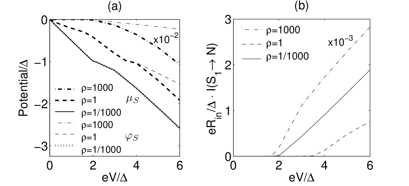
Figure 2: (a) Chemical and electrostatic potentials of the superconducting island as a function of bias voltage. (b) $I-V$ curves for different $\rho$. For clarity, in the case $\rho=1000$ the potentials have been multiplied by the factor 100 and the currents by the factor 1000.

Under the conditions formulated in Sect. II when the inelastic relaxation can be neglected, $\eta\gg\tau_{\rm e-e}^{-1}$, the kinetic equations (7) and (8) were solved numerically for nonequilibrium distributions in both normal and superconducting islands. Throughout numerical computations we use the value of the pair-breaking parameter $\Delta/\gamma=1000$. For nonequilibrium states, the bath temperature was fixed at a value much lower than the gap, $T_{\rm bath}=(0.1/1.764)\,\Delta$. This corresponds to $T=0.1\,T_{c}$ if the gap coincides with the zero-temperature BCS value $\Delta_{0}=1.764\,T_{c}$.

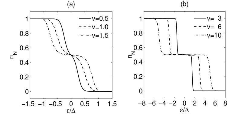
Figure 3: Nonequilibrium normal-island distributions for $\rho=1000$. We put $v\equiv eV/\Delta$ here and in Figs. 4–7 below.

The distribution functions in both N and S islands are in turn determined by the chemical potential of superconducting islands $\mu_{S}$ which was calculated self-consistently using the current conservation as discussed in the previous section. Chemical potential and the current–voltage curves are shown in Fig. 2.

We find three qualitatively distinct cases characterized by the ratio $\rho\equiv R_{\rm out}/R_{\rm in}$. For the ratio as large as $\rho=1000$, the distribution in the normal island, $n_{N}$, is shown in Fig. 3 for several values of $V$. Under biasing $V$, the distribution is driven into nonequilibrium. At first, this is seen only as a slight deviation from the Fermi function $n_{F}$ but for voltages $V/\Delta\gtrsim 1$, the distribution $n_{N}$ assumes the characteristic step-like profile. This behavior of $n_{N}$ can be explained as follows. For very high ratios $\rho$, the superconducting chemical potential is small: $\mu_{S}/eV\ll 1$ [compare with Fig. 2 (a)]. The kinetic equations (7), (8) yield then $f_{1}(N)\approx f_{1}(S)\approx f_{1}(N_{1})$. Since $f_{2}(N)=0$, one has $2n_{N}=1-f_{1}(N)=1-f_{1}(N_{1})$. The external leads $N_{1}$ and $N_{2}$ are in equilibrium such that $f_{1}(N_{1})=-n_{F}(\epsilon-eV)+n_{F}(-\epsilon-eV)$. Thus, $n_{N}=[n_{F}(\epsilon-eV)+n_{F}(\epsilon+eV)]/2$. Since $f_{2}(S)$ is small due to the high resistivity ratio, one has also $n_{S}\approx n_{N}$ for the superconducting island.

The distributions for the ratios $\rho=1$ and $\rho=1/1000$ are shown in Figs. 4 and 5. They also change their shape strongly above a certain voltage. The changes correspond to the sharp rise in the electric current through the junction, Fig. 2(b). The origin of this behavior is discussed in connection with the charge imbalance, see next subsection. The distribution functions of the N island show a cooling behavior: The distribution becomes very steep, thus corresponding to a low effective electron temperature at such bias voltages when the chemical potential difference across the superconductor/normal-island junction is $|\mu_{S}|\approx\Delta$. One can define an effective temperature through Pekola2

$$k_{B}T_{\rm eff}=\frac{\sqrt{6}}{\pi}\sqrt{\int_{0}^{\infty}\left[1-f_{1,\epsilon}(N)\right]\epsilon\,d\epsilon}\quad.$$ (32)

keeping in mind that $f_{2}(N)=0$ for the center N island. This definition gives the actual electron temperature in (quasi)equilibrium. The effective temperatures have minima for $\rho\lesssim 1$ as seen in Fig. 6.

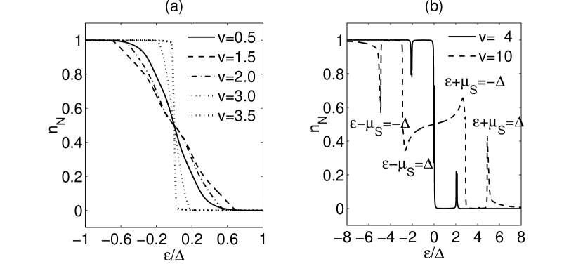
Figure 4: Nonequilibrium normal metal distributions for $\rho=1$.

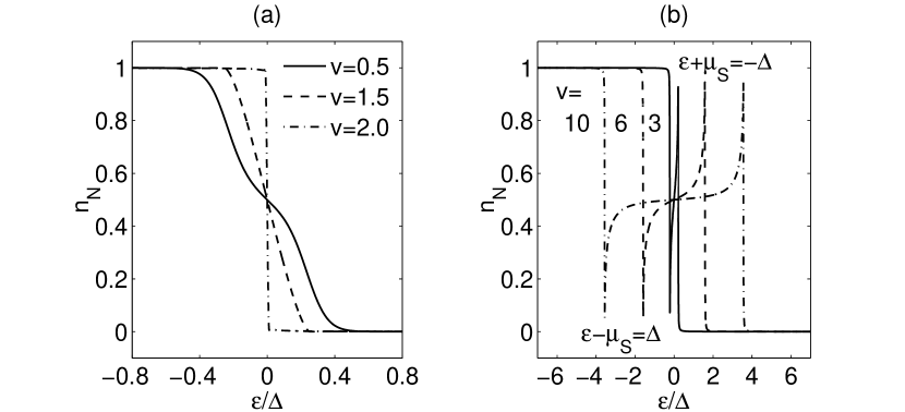
Figure 5: Nonequilibrium normal metal distributions for $\rho=1/1000$.

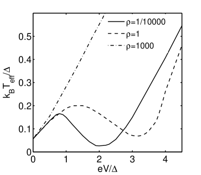
Figure 6: Effective temperature $T_{\rm eff}$ of Eq. (32).

For a good contact between the outer normal electrodes and the superconductors S, i.e. when $\rho=1/1000$, there is no deviation between the superconductor distribution function $n_{S}$ and that in the normal reservoir, a Fermi function with $\varphi_{N_{1}}=V/2$. This suggests that, for small $\rho$, the considered structure is similar to a SINIS system with superconducting reservoirs. The distribution in the central N island for low $\rho$ is shown in Fig. 5. It resembles the distribution found for a SINIS structure Giazotto .

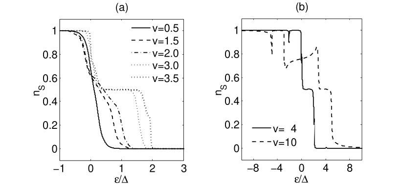
Figure 7: Nonequilibrium superconductor distributions for various bias voltages when $\rho=1$.

When the ratio $\rho$ increases, the distribution in the superconductors, $n_{S}$, deviates from the Fermi function as shown in Fig. 7. Nonequilibrium distribution in the superconducting regions on both sides of the central normal island drives the state in the N island yet further from equilibrium, see Fig. 4. For larger $\rho$ the cooling behavior becomes less pronounced and finally disappears, see Fig. 6.

For low and intermediate values of $\rho$, we observe novel features of highly nonequilibrium distributions both in the central normal and in the side superconducting islands. For small $\rho=1/1000$, peaks in the energy distribution appear at energies $\pm\epsilon=\Delta+\mu_{S}$ (see Fig. 5). In addition to these, new peaks appear in Fig. 4 for larger $\rho=1$ at energies $\pm\epsilon=-\Delta+\mu_{S}$, for voltages considerably exceeding $\Delta/e$. Both sets of peaks come as a result of recursion from singularities in $g_{\epsilon}$ and $F_{\epsilon}$ at $\epsilon=\pm\Delta$ in the kinetic equations. The new peaks at $\pm\epsilon=-\Delta+\mu_{S}$ are present as long as the distribution functions of the two reservoirs differ at the corresponding energies and appear as a result of suppression of the distribution function due to a large factor $(\Delta/\gamma)F_{\epsilon\pm\mu_{S}}$ in the sub-gap region in Eqs. (21) and (22). Thus, the requirement of the new peaks is roughly $\Delta-\mu_{S}<eV/2$ which can be fulfilled if $\mu_{S}\neq-eV/2$ as is the case for intermediate values of $\rho$.

V.1.2 Charge imbalance

As mentioned above, the distribution function of the center N island suffers a drastic change above a certain voltage. This change coincides with the upturn of the current as a function of the applied voltage in Fig. 2(b) and is accompanied by a deviation of the chemical potential $\mu_{S}$ from the electric potential $-e\varphi_{S}$ in the adjacent superconductor as determined by Eq. (31). In equilibrium, their difference $\Phi=0$. In nonequilibrium, a difference between $\mu_{S}$ and $-e\varphi_{S}$ appears according to Fig. 2(a). The singularities appear when the chemical potential difference between the superconductor and one of the contacting normal conductors approaches $\Delta$. This corresponds to $eV\sim 2\Delta$ for a large mismatch between $R_{\rm in}$ and $R_{\rm out}$ or to $eV/2\sim 2\Delta$ for $R_{\rm in}=R_{\rm out}$. To measure potentials $\varphi_{S}$, a capacitive connection would be required, in addition to the usual resistive connection only capable of detecting $\mu_{S}$.

For a good contact between the outer normal electrodes and the superconductors S, i.e. when $\rho=1/1000$, there is no deviation between $-e\varphi_{S}$ and $\mu_{S}$. This can be understood by considering the function $n_{S}$, which coincides essentially with a Fermi function shifted by $\mu_{S}\approx-e\varphi_{N_{1}}=-eV/2$. For a Fermi function, $n_{\epsilon}=1-n_{-\epsilon}$, and the term in the brackets in Eq. (31) vanishes.

V.1.3 Gap instability

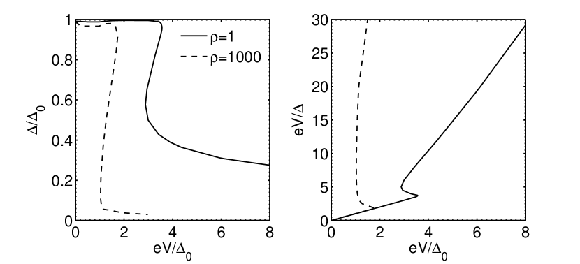
Figure 8: (a) Gap $\Delta$ as a function of bias voltage for two resistance ratios $\rho=1000$ (dashed line) and $\rho=1$ (solid line). Both quantities are normalized to zero-temperature BCS gap $\Delta_{0}$. (b) Conversion between $eV/\Delta$ and $eV/\Delta_{0}$ for $\rho=1000$ (dashed line) and $\rho=1$ (solid line).

In a nonequilibrium state, the gap function $\Delta$ has to be calculated self-consistently using Eq. (27). Employing the equation for the critical temperature $T_{c}$,

$$\frac{1}{\lambda}=\int_{0}^{E_{c}}\tanh\frac{\epsilon}{2T_{c}}\,\frac{d\epsilon}{\epsilon},$$ (33)

one can exclude the interaction constant in favor of $T_{c}$. For a low resistance ratio $\rho=1/1000$, the gap does not change considerably, $\Delta\approx\Delta_{0}$ for all $V$, $\Delta_{0}=1.764\,T_{c}$ being the zero-temperature BCS gap. However, for a higher resistance ratio, the nonequilibrium energy gap is modified dramatically as shown in Fig. 8(a). One observes a drastic change in the gap for voltages coinciding with those where the change in the distribution is seen. The energy gap becomes a multi-valued function which implies hysteretic behavior accompanied by jumps of $\Delta$ at the corresponding voltages. For a very poor contact between the superconducting islands and the outer normal reservoirs, i.e. for high $\rho$ when deviation from equilibrium is the largest, the gap function jumps down to very small values and superconductivity is nearly destroyed. For a lower tunnel resistance ratio $\rho$, the gap decrease is not so huge and superconductivity is less suppressed. Note that with respect to the order parameter magnitude, the bath temperature chosen for our calculations can be considered as zero. Indeed, the temperature was set much lower than $\Delta$ while the relevant energy scales for the distribution function are determined by the applied voltage and by $\Delta$ itself. Thus the thermal effects on the gap are negligible.

The predicted suppression of superconductivity in a nonequilibrium superconductor placed into a tunnel contact with a nonequilibrium normal-metal electrode contrasts to the superconductivity enhancement observed in tunnel SIS^′IS structures SCenhancement1 ; SCenhancement2 ; HeslingaKlapwijk where the nonequilibrium superconductor is in contact with equilibrium superconducting electrodes.

Note that since in our calculations we normalize all the values with the dimensions of energy (like voltage, excitation energy, temperature) to the real gap magnitude $\Delta$, we need to rescale the real voltage to its relative magnitude. Conversion between the relative, $V/\Delta$, and the real voltage normalized to the BCS gap, $V/\Delta_{0}$, is provided by Fig. 8(b) where the graphs are given for $\rho=1000$ and $\rho=1$. As seen from Fig. 8(b), for $\rho=1$ high relative voltages $eV/\Delta$ can be achieved for comparatively low absolute voltage values $eV/\Delta_{0}$.

V.1.4 Visualization

The peaks in the distribution of N and S islands can be monitored by measuring the differential conductance of a probe tunnel SINIS or SIS^′IS junction attached to the island in question. Let us consider a SINIS probe junction attached to the central N island as in Ref. Pekola2, . The distribution function in the N island is not modified by the measuring current if the tunnel resistance of the probe junction satisfies $R_{S_{P}N}\gg R_{\rm in}+R_{\rm out}$. The current through the probe junction is

$$I(N\rightarrow S_{P}) = -\frac{1}{eR_{S_{P}N}}\int_{-\infty}^{\infty}g_{\epsilon}(S_{P})$$

$$\times\left[n_{F}(\epsilon)-n_{N}(\epsilon+eV_{P}/2)\right]\,d\epsilon,$$

where the bulk superconducting probe electrode S_P is assumed to be in equilibrium with a potential $\varphi_{P}$ so that $\mu_{S_{P}}=-e\varphi_{P}=-eV_{P}/2$ where $V_{P}$ is the voltage between the two probe electrodes. The energy gap $\Delta_{P}$ in the probe electrodes is assumed to have the magnitude corresponding to the BCS value for $T=T_{\rm bath}$. As $T_{\rm bath}\approx 0.1\,T_{c}$, the gap $\Delta_{P}$ is very close to $\Delta_{0}$. In addition, we set $\gamma_{P}=\gamma$ for the depairing rate in the probe electrodes. The differential conductance becomes

$$\frac{dI}{dV_{P}}=\frac{1}{2R_{S_{P}N}}\int_{-\infty}^{\infty}g_{\epsilon}(S_{P})\frac{dn_{N}(\epsilon+eV_{P}/2)}{d\epsilon}\,d\epsilon\ .$$ (34)

Due to the peaks in $g_{\epsilon}(S_{P})$ at $\epsilon=\pm\Delta_{P}$, the differential conductance should reproduce the peaks in the distribution function $n_{N}$ at the probe voltages satisfying $\epsilon\pm\Delta_{P}=V_{P}/2$.

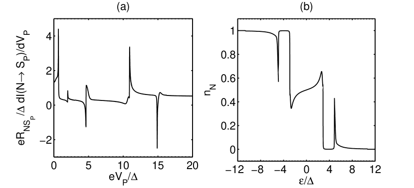
Figure 9: Differential conductance for the probe junction (a) and the corresponding quasiparticle energy distribution in the normal-metal island (b) when $\rho=1,eV/\Delta=10$.

The differential conductance $dI(N\rightarrow S_{P})/dV_{P}$ together with the corresponding distributions in the central normal island for $eV/\Delta=10$ are shown in Fig. 9 for the ratio $\rho=1$. The peaks in the distribution in Fig. 9(b) are located at $\epsilon=\pm\Delta-\mu_{S}$, i.e., $\epsilon=2.89\,\Delta$ and $\epsilon=4.89\,\Delta$. Two more are located at $\epsilon=\pm\Delta-3\mu_{S}$ or $\epsilon=10.7\,\Delta$ and $\epsilon=12.7\,\Delta$ (out of scale in Fig 9(b)). Comparing these to the locations of the larger peaks in Fig. 9(a) and using the $\Delta$-vs-$\Delta_{0}$ conversion curve of Fig. 8(a) we see that the peaks in the distribution are indeed reproduced at the probe voltage $eV_{P}/\Delta=2\epsilon/\Delta\pm 2\Delta_{P}/\Delta$. The smaller peaks in Fig. 9(a) refer to the less pronounced structure in the distribution not well-resolved in Fig. 9(b).

V.2 Quasi-equilibrium

As discussed in Section II, the condition for full nonequilibrium is $\eta\gg\tau_{\rm inel}^{-1}$, where $\eta$ is defined according to Eq. (2). The inelastic relaxation may be further separated to relaxation caused by electron–electron and electron–phonon interactions with collision rates $\tau_{\rm e-e}^{-1}$ and $\tau_{\rm e-ph}^{-1}$, respectively. The experimental situation in nanoscale heterostructuresPekola2 corresponds often to the case $\tau_{\rm e-e}^{-1}>\tau_{\rm e-ph}^{-1}$. In particular, the limit of low coupling to the heat bath in S and/or N islands is frequently realized when the tunnel injection rate is intermediate between the electron–phonon and electron–electron relaxation rates, $\tau_{\rm e-ph}^{-1}\ll\eta\ll\tau_{\rm e-e}^{-1}$. We refer to this case as quasi-equilibrium. While the near absence of electron–phonon interactions prohibits the quasiparticles from coupling to the lattice, the rate of electron–electron scattering is high enough for the quasiparticles to assume a Fermi distribution with certain electron temperature. We have studied the cooling performance of our NISINISIN heterostructure in the quasi-equilibrium limit looking at the electron temperature of the central N island.

We note that the simple expressions for the regular Green functions of the form of Eqs. (23) and (24) are not applicable in the strict sense when the inelastic relaxation dominates. To find the exact expressions for the regular Green functions one has to solve the Eilenberger equations (14), (15) with the proper inelastic collision integrals. However, to simplify our problem, we model the pair breaking effects of inelastic relaxation by an effective pair-breaking rate $\gamma$ in Eqs. (23) and (24) in the same way as for the tunnel limit described in the previous sections. This approximation is frequently used in practical calculations. Here we put $\Delta/\gamma=1000$ as above.

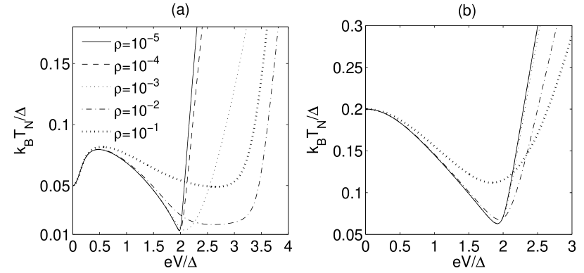
Figure 10: Temperature in the normal-metal island as a function of bias voltage for bath temperatures 0.05$\,\Delta$ (a) and 0.2$\,\Delta$ (b) when the system is quasiequilibrium.

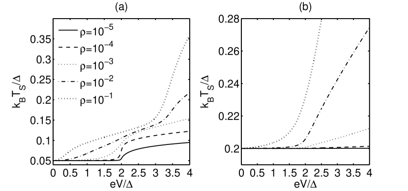
Figure 11: Temperature in the superconductor as a function of bias voltage for bath temperatures 0.05$\,\Delta$ (a) and 0.2$\,\Delta$ (b) when the system is quasiequilibrium.

Applying the tunnelling model shows that depending on the configuration of the quasiparticle traps, i.e. the ratio of outer and inner junction resistances $\rho$, effective cooling of the normal-metal island can be achieved as demonstrated also in Ref. Pekola2, . The temperatures of the central N island and of the contacting S island are shown in Figs. 10 and 11, respectively. The temperature of N island indeed displays a minimum below bath temperature when the ratio $\rho$ is small. However, for large $\rho$, the temperature monotonously rises above the bath temperature with an increasing voltage. As can be deduced from Figs. 10 and 11, the cooling effect is not attributed to the presence of two additional normal metal reservoirs. On the contrary, smallest ratio $\rho$, which corresponds to the strongest cooling, is seen to lead to almost constant $T_{S}=T_{\rm bath}$ as it would be the case for pure superconducting reservoirs. Another remark concerns the cooling efficiency of a NISINISIN configuration as $T_{\rm bath}$ is lowered. Indeed, for $T_{\rm bath}=0.2\,\Delta$ the temperature minimum for the depairing parameter $\gamma=\Delta/1000$ used for our calculations is roughly $0.063\,\Delta$ while the minimum is $T_{\rm min}=0.024\,\Delta$ for $T_{\rm bath}=0.15\Delta$, and it is $T_{\rm min}\approx 0.013\,\Delta$ for $T_{\rm bath}\leq 0.1\,\Delta$. From the numerical results in the case $1\gg\rho\gtrsim\gamma/\Delta$, we find that the minimum achieved temperature follows $T_{\rm min}/T_{c}\approx 0.24\rho^{\zeta}$ where $\zeta\approx 0.5$. For smaller $R_{\rm out}$, the minimum temperature $T_{\rm min}$ is determined by the inverse proximity effect described by the depairing parameter $\gamma$ (see Ref. Pekola2, ). Combining both the superconductor heating due to a finite $R_{\rm out}$ and the effects of depairing, we can write an approximate formula for the minimum temperature for relatively low bath temperatures,

$$T_{\rm min}/T_{c}=2.5\left(\gamma/\Delta\right)^{2/3}+0.24\rho^{1/2}\ .$$ (35)

For $\rho\ll 1$, the depairing rate $\gamma$ is limited by $R_{\rm out}$, i.e., $\gamma=1/(4\nu_{S}e^{2}\Omega_{S}R_{\rm out})=(r_{S}/2R_{\rm out})E_{T}$, where $E_{T}=D/L^{2}$ is the Thouless energy in the superconducting island with length $L$ and $r_{S}$ is its resistance. Substituting this into Eq. (35), we find that the minimum temperature is optimized with

$$\rho\approx 6.4\left[(E_{T}/\Delta)(r_{S}/R_{\rm in})\right]^{4/7}\ .$$ (36)

Note, however, that Eq. (36) is valid provided $r_{S}/R_{\rm in}\ll\rho\ll 1$.

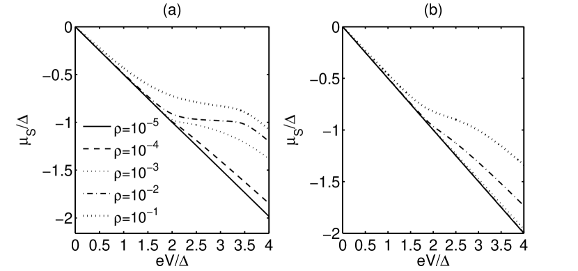
Figure 12: Chemical potential of the superconductor as a function of bias voltage for bath temperatures 0.05$\,\Delta$ (a) and 0.2$\,\Delta$ (b) when the system is in quasiequilibrium.

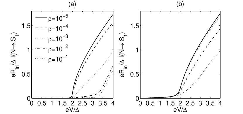
Figure 13: Electric current between S and N islands as a function of bias voltage for bath temperatures 0.05$\,\Delta$ (a) and 0.2$\,\Delta$ (b) when the system is in quasiequilibrium.

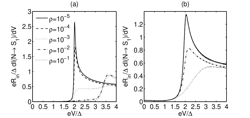
Figure 14: Differential conductance as a function of bias voltage for bath temperatures 0.05$\,\Delta$ (a) and 0.2$\,\Delta$ (b) when the system is in quasiequilibrium.

The sharp rise in $T_{N}$ and $T_{S}$ occurs generally around $V=2\,\Delta$ but for larger values of $\rho$, when also $T_{\rm bath}\rightarrow T_{\rm min}$, the upturn shifts towards higher voltages $V$. This is because the upturn is determined by the condition $-\mu_{S}\approx\Delta$ rather than $V/2=\Delta$ as can be seen by comparing Figs. 10 and 11 to Fig. 12. For increasing bath temperature, though, this trend is smeared and disappears. The voltages corresponding to the temperature rise are also seen in the IV-curves in Fig. 13 and in the differential conductance, Fig. 14.

VI Discussion

VI.1 Electron cooling

According to our results, the electron cooling is the most effective when the outer resistance is low $\rho\ll 1$. In fact, both the effective temperature and the distribution function in the superconducting region almost coincide with those in the bath for such voltages that yield $|\mu_{s}|<\Delta$ especially for very low ratios of $\rho$. When the ratio $\rho$ is low, a good contact between the inner superconducting region and the outer electrode makes the distributions in these two regions not so much different from each other, thus decreasing the role of the extra junction. This conclusion is valid only within the tunneling approximation. When the contact between the outer electrodes and superconducting islands are more transparent, cooling properties of the device are affected by the inverse proximity effect from the external normal leads.

For larger ratios $\rho$, the extra junction prevents the state of the superconducting region from reaching equilibrium, thus reducing the cooling power of the entire structure. Moreover, this limit has another disadvantage as far as the cooling performance is concerned: For larger voltages when $eV$ approaches $2\Delta$, one expects a suppression of superconductivity in the $S$ regions down to lower values of $\Delta$ and thus the cooler would become even less effective. This suggests that the cooling performance of an NISINISIN structure cannot be improved essentially by an extra tunnel junction as compared to that of a simple SINIS structure. However, the presence of the quasiparticle traps helps to practically realize the superconducting reservoirs by thermalizing them quickly to an object with a high thermal conductance.

VI.2 Nonequilibrium distribution

Nonequilibrium distribution formed in the superconducting islands for high values of $\rho$ results in yet stronger deviation from equilibrium in the central normal island. As seen from Figs. 4 and 5, the distribution function in the N island is characterized by peaks at energies $\pm\epsilon=\Delta\pm\mu_{s}$, and also $\pm\epsilon=\Delta\pm 3\mu_{s}$, etc., for voltages considerably exceeding $\Delta/e$. These peaks are clearly visible in the differential conductance of a probe tunnel SINIS junction made at the central normal island, Fig. 9. Simultaneously, nonequilibrium states in the superconducting region follow the gap which is strongly reduced as compared to its equilibrium BCS value $\Delta_{0}$. The transition into a nonequilibrium state is accompanied by a jump in the gap magnitude which leads to the jump in the relative voltage: high values of $eV/\Delta$ can be reached already for not very large absolute values of voltage $eV/\Delta_{0}$. This makes observation of the nonequilibrium states in N and S regions more easily accessible in experiments.

- (1) M. Nahum, T. M. Eiles, and J. M. Martinis, Appl. Phys. Lett. 65, 3123 (1994).
- (2) M. M. Leivo, J. P. Pekola, and D. V. Averin, Appl. Phys. Lett. 68, 1996 (1996).
- (3) D. Golubev and A. Vasenko, in: International Workshop on Superconducting Nano-electronics Devices, edited by J. Pekola, B. Ruggiero, and P. Silvestrini (Kluwer Academic/Plenum Publishers, New York, 2002), p. 165.
- (4) J.P. Pekola, T.T. Heikkilä, A.M. Savin, J.T. Flyktman, F. Giazotto, and F.W.J. Hekking, Phys. Rev. Lett. 92, 056804 (2004).
- (5) D.R. Heslinga and T.M. Klapwijk, Phys. Rev. B 47, 5157 (1993).
- (6) V.M. Dmitriev, V.N. Gubankov, and F.Y. Nad’, in Nonequilibrium superconductivity, D.N. Langenberg and A.I. Larkin eds. (North Holland, Amsterdam, 1986) p. 163; G.M. Eliashberg and B.I. Ivlev, in ibid, p.211.
- (7) M.G. Blamire, E.C.G. Kirk, J.E. Evetts, and T.M. Klapwijk, Phys. Rev. Lett. 66, 220 (1991).
- (8) H. Pothier, S. Guéron, N. O. Birge, D. Esteve, and M.H. Devoret, Phys. Rev. Lett. 79, 3490 (1997).
- (9) F. Giazotto, T.T. Heikkilä, F. Taddei, R. Fazio, J.P. Pekola, and F. Beltram, Phys. Rev. Lett. 92, 137001 (2004).
- (10) J.P. Pekola, D.V. Anghel, T.I. Suppula, J.K. Suoknuuti, A.J. Manninen, and M. Manninen, Appl. Phys. Lett. 76, 2782 (2000).
- (11) A. Brinkman, A.A. Golubov, H. Rogalla, F.K. Wilhelm, and M.Yu. Kupriyanov, Phys. Rev. B 68, 224513 (2003).
- (12) N.B. Kopnin, Theory of Nonequilibrium Superconductivity (Clarendon, Oxford, 2001).