Quantum Monte Carlo based on two-body density functional theory for fermionic many-body systems: application to ³He

Abstract

We construct a quantum Monte Carlo algorithm for interacting fermions using the two-body density as the fundamental quantity. The central idea is mapping the interacting fermionic system onto an auxiliary system of interacting bosons. The correction term is approximated using correlated wave-functions for the interacting system, resulting in an effective potential that represents the nodal surface. We calculate the properties of ³He and find good agreement with experiment and with other theoretical work. In particular our results for the total energy agree well with other calculations where the same approximations were implemented but the standard quantum Monte Carlo algorithm was used.

Density-functional theory Hohenberg64 ; Kohn65 (DFT) and quantum Monte Carlo Anderson75 ; Foulkes01 (QMC) are generally thought of as two distinct approaches to the problem of interacting fermions. DFT is based on the Hohenberg-Kohn theorems Hohenberg64 (HK) which state that the energy of an interacting fermion system in an external field can be written as a functional of the density, and that minimizing the energy as a functional of the density gives the ground state energy (HK theorems). Applications of DFT are usually based on the Kohn and Sham Kohn65 method, where an auxiliary noninteracting system is invoked. Minimization is achieved with respect to the orbitals of the auxiliary system. QMC also involves minimization of the energy. One way of minimizing, is to propagate a trial wavefunction in imaginary time Anderson75 , so that it asymptotically approaches the ground state.

In this letter we present a QMC method derived from an extension of DFT where the two-body density ($n^{(2)}$) is the fundamental quantity Ziesche96 ; Levy01 . As in standard DFT the energy functional is universal but unknown, thus approximations schemes are necessary. In the spirit of the Kohn-Sham ansatz we invoke an auxiliary system with identical $n^{(2)}$ as the system of interacting fermions under investigation, but instead of a non-interacting system, one of interacting bosons. As in the Kohn-Sham method, minimization is not performed with respect to the density, but with respect to the bosonic wavefunction via QMC Anderson75 . This can be done, since the two-body density can be written in terms of the bosonic wavefunction. In our method the sign-problem does not arise explicitly, thus fixed-node Reynolds82 (FN) or released-node Ceperley80 (RN) techniques are not needed. In the auxiliary fields Monte Carlo method Baer98 the need for FN or RN is also circumvented, but the sign-problem still manifests in the phases of the auxiliary fields.

The correction term necessitated by our ansatz is obtained approximately using correlated basis functions. The resulting approximation consists of a two-body and a three-body potential (effective nodal surface). The appearance of the three-body potential (and density) in our energy functional is a result of our approximation scheme. In principle our approximate energy functional can still be written as a functional of $n^{(2)}$, since according to the HK theorems Hohenberg64 the three-body density (as all other observables) is a functional of $n^{(2)}$. As far as the method developed here is concerned, the minimization itself is performed with respect to the bosonic wavefunction, thus higher-order potentials are easily handled.

We apply our formalism to calculate the total energy, potential energy, and the structure factor of ³He in a range of densities close to the equilibrium one ($\rho_{0}=0.273N/\sigma^{-3}$, $\sigma=2.556$ Å). Our model estimates the density that minimizes the total energy to be slightly less than the experimental result, as one would expect from the fact that we are not including back-flow effects. The calculated energies are in very good agreement with QMC results at the same level of approximation, and compare reasonably well with experiment.

Given a system of interacting particles with potential $w$ (including two-body and one-body potentials) and with two-body density $n^{(2)}$ (the diagonal elements of the two-body density matrix) HK can be extended as follows:

• There is a one to one correspondence between $w$ and $n^{(2)}$.

• The ground state energy of the system can be obtained by minimizing $E$ as a function of $n^{(2)}$.

The proof of these statements is an easy extension of the original work Hohenberg64 , and can be extended to $N$-representable two-body densities using the Levy-constrained search Levy79 . The energy (and all other observables) can be written as a functional of $n^{(2)}$ as

$$E[n^{(2)}]=T[n^{(2)}]+\int d{\bf r}d{\bf r}^{\prime}w({\bf r},{\bf r^{\prime}})n^{(2)}({\bf r},{\bf r^{\prime}}).$$ (1)

$T[n^{(2)}]$ is a universal functional of $n^{(2)}$, that is, the kinetic energy can be determined by knowing only $n^{(2)}$. Whether the system is composed of bosons or fermions enters only in the form of $T[n^{(2)}]$; the functional dependence of the potential energy term on $n^{(2)}$ is the same for bosons or fermions.

In the original DFT of HK, the universal functional includes the kinetic energy and the pair interaction and is a function of the one-body density ($F_{\mbox{\scriptsize{HK}}}[n]$). The analogue of $F_{\mbox{\scriptsize{HK}}}[n]$ in pair-density functional theory is simply the kinetic energy $T[n^{(2)}]$, i.e. it does not include any of the potential energy terms.

Figure 1: Effective exchange pair potential.

In order to obtain an applicable algorithm, we introduce an auxiliary system of interacting bosons, and add the required corrections. The issue of representability of a fermionic $n^{(2)}$ by a bosonic one shall be addressed in our extended study. Our starting equation is then

$$E_{\mbox{\scriptsize{F}}}[n^{(2)}]=T_{\mbox{\scriptsize{B}}}[n^{(2)}]+\Delta T[n^{(2)}]+\int d{\bf r}d{\bf r^{\prime}}w({\bf r},{\bf r^{\prime}})n^{(2)}({\bf r},{\bf r^{\prime}}),$$ (2)

where $T_{\mbox{\scriptsize{B}}}[n^{(2)}]$ is the kinetic energy of a system of bosons with two-body density $n^{(2)}$, and

$$\Delta T[n^{(2)}]=T_{\mbox{\scriptsize{F}}}[n^{(2)}]-T_{\mbox{\scriptsize{B}}}[n^{(2)}],$$ (3)

where $T_{\mbox{\scriptsize{F}}}[n^{(2)}]$ is the kinetic energy of a system of fermions with two-body density $n^{(2)}$.

The correction term in Eq. (3) is the difference between the kinetic energies of two systems identical $n^{(2)}$’s. differing only in that one is a system of fermions, the other a system of bosons. We develop an approximation to $\Delta T$ by constructing two trial wave-functions (one fermionic, one bosonic) with approximately equal $n^{(2)}$’s, and taking the difference of the kinetic energy expressions. The approximation presented here is valid for homogeneous systems.

For the fermionic one we take a wavefunction of the Jastrow-Slater form

$$\Psi_{\mbox{\scriptsize{F}}}=D^{\uparrow}D^{\downarrow}F,$$ (4)

where

$$F=\prod_{i<j}f(r_{ij}),$$ (5)

and where $D^{\uparrow}$($D^{\downarrow}$) indicates a Slater determinant of plane waves between atoms of spin up(down), and $f(r)$ is a correlation factor. In constructing a bosonic wavefunction with the same two-body density we take the same correlation factor as in Eq. (4), but to account for the determinants we multiply by additional correlation factors between parallel spins, i.e.

$$\Psi_{\mbox{\scriptsize{B}}}=F^{\uparrow}_{x}F^{\downarrow}_{x}F,$$ (6)

where

$$F^{\uparrow(\downarrow)}_{x}=\prod_{i<j}f^{\uparrow(\downarrow)}_{x}(r_{ij}),$$ (7)

where the product in Eq. (7) indicates a multiplication between pairs of parallel spins. The correlation factors $f^{\uparrow(\downarrow)}_{x}(r)$ should be chosen in such a way that the two-body densities obtained from Eqs. (4) and (6) are identical. The correction term in this case can be explicitly obtained

$$\Delta T[n^{(2)}]=T_{0}+\sum_{i}\frac{1}{2mN_{\mbox{\scriptsize{F}}}}\int d{\bf R}|D^{\uparrow}D^{\downarrow}|^{2}\nabla_{i}F\cdot\nabla_{i}F$$

$$-\sum_{i}\frac{1}{2mN_{\mbox{\scriptsize{B}}}}\int d{\bf R}|F^{\uparrow}_{x}F^{\downarrow}_{x}|^{2}\nabla_{i}F\cdot\nabla_{i}F$$

$$+\sum_{i}\frac{1}{2mN_{\mbox{\scriptsize{F}}}}\int d{\bf R}F^{2}(F^{\uparrow}_{x}F^{\downarrow}_{x}\nabla_{i}^{2}F^{\uparrow}_{x}F^{\downarrow}_{x}),$$ (8)

where ${\bf R}$ denotes all coordinates, $m$ denotes the mass, and $N_{\mbox{\scriptsize{F}}},N_{\mbox{\scriptsize{B}}}$ are normalization integrals. $T_{0}=3/5k_{\mbox{\scriptsize{F}}}^{2}/(2m)$, which is the kinetic energy of the homogeneous non-interacting system ($k_{\mbox{\scriptsize{F}}}$ is the Fermi wave vector). If the correlation factor $f_{x}$ is chosen such that the two-body and three-body densities obtained from the determinants in Eq. (4) are identical to those obtained from the correlation factors $f_{x}$ in Eq. (6) then the second and third terms in Eq. (8) cancel resulting in

$$\Delta T[n^{(2)}]=T_{0}+\sum_{i}\frac{1}{2mN_{\mbox{\scriptsize{F}}}}\int d{\bf R}F^{2}(F^{\uparrow}_{x}F^{\downarrow}_{x}\nabla_{i}^{2}F^{\uparrow}_{x}F^{\downarrow}_{x}),$$ (9)

In obtaining a first approximation to the correlation term $f^{\uparrow(\downarrow)}_{x}$ in the case of a homogeneous system we can make use of the radial distribution function of the noninteracting fermion gas, given by

$$g_{x}(r)=1-\left\{\frac{3}{k_{\mbox{\scriptsize{F}}}^{3}r^{3}}(\mbox{sin}k_{\mbox{\scriptsize{F}}}r-k_{\mbox{\scriptsize{F}}}r\mbox{cos}k_{\mbox{\scriptsize{F}}}r)\right\}^{2}$$ (10)

We obtain $f_{x}$ from an inverse hypernetted chain equation (we also tried using $f_{x}=g_{x}$, and obtained very similar results). While $f^{\uparrow(\downarrow)}_{x}$ does not guarantee that the second and third terms in Eq. (8) will cancel, in this work we assume Eq. (9) as the form for our approximation. Thus the correction term resulting from Eq. (9) in our scheme is the sum of a two-body and a three-body interaction,

$$w^{(2)}_{x}(r)=\frac{1}{2m}\left\{\frac{\partial^{2}\mbox{ln}f_{x}(r)}{\partial r^{2}}+\frac{2}{r}\frac{\partial\mbox{ln}f_{x}(r)}{\partial r}\right\}$$

$$w^{(3)}_{x}(r_{12},r_{13})=\frac{1}{2m}(\nabla_{1}\mbox{ln}f_{x}(r_{12})\cdot\nabla_{1}\mbox{ln}f_{x}(r_{13})),$$ (11)

and a constant term $T_{0}$. The expressions are the same for both $f_{x}^{\uparrow}$, $f_{x}^{\downarrow}$, however in general $f_{x}^{\uparrow}\neq f_{x}^{\downarrow}$. Since in this work we will deal with the unpolarized case, where $f_{x}^{\uparrow}=f_{x}^{\downarrow}$ from now on we will drop the arrows.

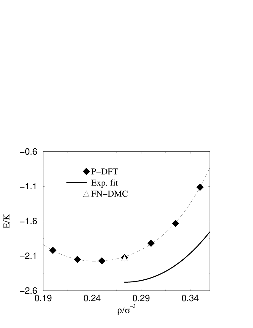
Figure 2: Total energy for ³He as a function of density. The solid curve is a fit to experimental results (Ref. Aziz73, ), the curve connecting our calculated points is a fifth order polynomial fit. The triangle is the result from a fixed node DMC calculation without backflow (Ref.Casulleras00, ).

Going beyond the weak coupling approximation would lead to correction terms including the correlation factor $f$. In principle $f$ is a functional of the two-body density of the system, thus a self-consistent algorithm would be necessary. Possibly this can be avoided by using known correlation factors for a given system under investigation (or obtaining one from solving the Euler equation Moroni95 ). Potentially, better approximations can also be obtained for $\Delta T$ if better wavefunctions are chosen in Eqs. (4) and (6). In our scheme three-body correlations and Feynman-Cohen back-flow Feynman56 have not been considered.

As a test of the quality of $f_{x}$ we have performed a Monte Carlo simulation at the experimental density ($\rho_{0}=0.273N/\sigma^{-3}$), and have found that the radial distribution function obtained is in good agreement with that of the noninteracting Fermi gas. Obviously, in this case the energies between the fermionic system and the auxiliary bosonic one correspond. In Fig. 1 the effective pair potential that incorporates the nodal surface (-$w^{(2)}_{x}$) is shown at $\rho_{0}$. The potential is an effective way of including the nodal structure, it is repulsive at short distances, and displays alternating valleys and barriers of decreasing magnitude.

We applied the above procedure to a system of unpolarized ³He atoms at zero temperature. We have used the HFD-HE2 interaction potential due to Aziz et al Aziz79 . Between particles with parallel spin the potential interaction modified by the additive terms given in Eq. (9). To reduce the variance in DMC we have used a guiding function of the form given in Eq. (6) with $f(r)=\mbox{exp}-b^{5}/2r^{5}$ ($b=1.15\sigma$, where $\sigma=2.556$ Å). The parameter $b$ was optimized by a variational Monte Carlo calculation. For other calculations on the same system see Refs. Lee81, ; Schmidt81, ; Panoff89, ; Moroni95, ; Casulleras00, .

We perform a series of calculations using the standard bosonic DMCAnderson75 algorithm. Our cell included 108 particles in all cases, we used an imaginary time step of 50 a.u. We collected averages over 100,000 steps. Total energies are estimated in the standard way, coordinate dependent observables were estimated using pure estimators Casulleras95 . The non-coordinate dependent part of the fermionic kinetic energy was obtained by subtracting from the total energy the potential and the correction term in Eq. (11).

$\rho/N\sigma^{-3}$	E	V	T	$\Delta$ T - T0
$0.2$	$-2.050(5)$	$-9.83(4)$	$7.78(4)$	$-1.040(4)$
$0.225$	$-2.174(6)$	$-11.25(4)$	$9.08(4)$	$-1.143(5)$
$0.25$	$-2.220(6)$	$-12.73(3)$	$10.51(4)$	$-1.253(1)$
$0.273$	$-2.147(7)$	$-14.03(3)$	$11.89(4)$	$-1.341(3)$
$0.3$	$-1.944(8)$	$-15.67(4)$	$13.73(4)$	$-1.521(4)$
$0.325$	$-1.65(1)$	$-17.09(7)$	$15.44(8)$	$-1.521(4)$
$0.35$	$-1.17(1)$	$-18.62(5)$	$17.45(6)$	$-1.642(5)$

Table 1: Energy quantities per particle as a function of density. All data are in Kelvin.

In Fig. 2 we compare our calculated total energies with experimental results. The thick solid curve is a fit to experimental results Aziz73 . The minimum density obtained by us is in close agreement with the experimental result (exp:$0.273N\sigma^{-3}$,calc:$0.244N\sigma^{-3}$). The structure factor, shown in Fig. 3 also compares well with experiment. The experimental DeBruynOubuter87 minimum energy is $-2.473$ K, our calculated energy at that density is $-2.147(7)$ K. Our energy at the calculated minimum density (from the fitted curve) is $-2.220(6)$ K. It is important to note that our results are in good agreement with previous calculations that do not include the back-flow correction (in Ref. Casulleras00, a QMC calculation without back-flow is reported resulting in $-2.128(15)$ K for the total energy per particle). We are not aware of fixed-node DMC calculations without back-flow for the full density range presented here, but variational Monte Carlo Schmidt81 ; Moroni95 calculations indicate that the nedlect of back-flow corrections leads to an over-estimation of the energy by a few tenths of a Kelvin (see Figure 1. in Ref. Schmidt81, ). Our calculated energies differ more from the experimental ones at higher densities. This is not surprising, since it is known that the back-flow approximation is more crucial at higher densities. Kwon98

Figure 3: Comparison of calculated (solid triangles) and experimental (circles: Ref. Achter69, and empty triangles: Ref. Hallock72, ) structure factor of ³He at equilibrium density.

In Table 1 we present values for the total, potential, kinetic energies, and for the coordinate dependent part of the correction term ($\Delta T-T_{0}$). Our value for the potential energy at $\rho_{0}$ ($-14.03(3)$ K) also compares reasonably well with other theoretical results ($\langle V\rangle=-14.84(10)$ K Panoff89 . The coordinate dependent part of $\Delta T$ gives only a small correction compared to the value of the kinetic energy itself (the bosonic kinetic energy plus $T_{0}$ is already a reasonable approximation to the kinetic energy). Thus using an auxiliary bosonic system is a promising scheme for developing approximations.

We have demonstrated that using an algorithm constructed from the pair-density a good description of an interacting fermionic system can be obtained. Our algorithm is arrived at by invoking an auxiliary system of bosons, therefore the calculation itself can be performed by a bosonic DMC algorithm. While it is clear that further work needs to be done to obtain a better approximation, the fact that we have obtained quantitative results for the observables calculated demonstrates that this avenue is worth pursuing. Our future directions include the developing and testing of more sophisticated approximations for the kinetic energy correction term used here, such as implementing back-flow, three-body correlation, and inverting the fermionic hypernetted-chain approximation Fantoni74 ; Krotscheck71 . Comparison of our method to related ones Reynolds82 ; Ceperley80 ; Baer98 is also of interest.

This research was supported by MIUR-2001/025/498 and by SISSA. We benefitted greatly from discussions with Professor K. E. Schmidt.

References

- (1) P. Hohenberg and W. Kohn Phys. Rev. 136B , 864 (1964).
- (2) W. Kohn and L. J. Sham Phys. Rev. 140 , A1133 (1965).
- (3) J. B. Anderson J. Chem. Phys. 63 , 1499 (1975).
- (4) W. M. C. Foulkes, L. Mitas, R. J. Needs, and G. Rajagopal Rev. Mod. Phys. 73, 33 (2001).
- (5) P. Ziesche, Int. J. Quantum Chem. 60, 149 (1996).
- (6) M. Levy and P. Ziesche, J. Chem. Phys. 115, 9110 (2001).
- (7) P. J. Reynolds, D. M. Ceperley, B. J. Alder, and W.A. Lester, J. Chem. Phys. 77, 5593 (1982).
- (8) D. M. Ceperley and B. J. Alder, Phys. Rev. Lett. 45, 566 (1980).
- (9) R. Baer, M. Head-Gordon, and D. Neuhauser, J. Chem. Phys. 109, 6219 (1998).
- (10) M. Levy, Proc. Nat. Acad. Sci. USA 76, 6062 (1979).
- (11) S. Moroni, S. Fantoni, and G. Senatore Phys. Rev. B 52, 13547 (1995).
- (12) R. P. Feynman and M. Cohen, Phys. Rev. 102, 1189 (1956).
- (13) R. A. Aziz, V. P. S. Nain, J. S. Carley, W. L. Taylor, and G. T. McConville, J. Chem. Phys. 70, 4331 (1979).
- (14) M. A. Lee, K. E. Schmidt, M. H. Kalos, and G. V. Chester, Phys. Rev. Lett. 46, 728 (1981).
- (15) K. E. Schmidt, M. A. Lee, M. H. Kalos, and G. V. Chester, Phys. Rev. Lett. 47, 807 (1981).
- (16) R. M. Panoff and J. Carlson, Phys. Rev. Lett. 62, 1130 (1989).
- (17) J. Casulleras and J. Boronat, Phys. Rev. Lett. 84, 3121 (2000).
- (18) J. Casulleras and J. Boronat, Phys. Rev. B 52, 3654 (1995).
- (19) R. A. Aziz, and R. K. Pathria, Phys. Rev. A 7, 809 (1973).
- (20) R. De Bruyn Ouboter and C. N. Yang Physica B & C 144, 127 (1987).
- (21) Y. Kwon, D. M. Ceperley, and R. M. Martin, Phys. Rev. B 58, 6800 (1998).
- (22) S. Fantoni and S. Rosati, Lett. Nuov. Cimento 10, 545 (1974).
- (23) E. Krotscheck and M. L. Ristig, Phys. Lett. A48, 17 (1971).
- (24) E. K. Achter and L. Meyer, Phys. Rev. 188, 291 (1969).
- (25) R. B. Hallock, J. Low Temp. Phys. 26, 109 (1972).