Two-Gaussian excitations model for the glass transition

Abstract

We develop a modified “two-state” model with Gaussian widths for the site energies of both ground and excited states, consistent with expectations for a disordered system. The thermodynamic properties of the system are analyzed in configuration space and found to bridge the gap between simple two state models (“logarithmic” model in configuration space) and the random energy model (“Gaussian” model in configuration space). The Kauzmann singularity given by the random energy model remains for very fragile liquids but is suppressed or eliminated for stronger liquids. The sharp form of constant volume heat capacity found by recent simulations for binary mixed Lennard Jones and soft sphere systems is reproduced by the model, as is the excess entropy and heat capacity of a variety of laboratory systems, strong and fragile. The ideal glass in all cases has a narrow Gaussian, almost invariant among molecular and atomic glassformers, while the excited state Gaussian depends on the system and its width plays a role in the thermodynamic fragility. The model predicts the existence of first-order phase transition for fragile liquids. The analysis of laboratory data for toluene and $o$-terphenyl indicates that fragile liquids resolve the Kauzmann paradox by a first-order transition from supercooled liquid to ideal glass state at a temperature between $T_{g}$ and Kauzmann temperature extrapolated from experimental data. We stress the importance of the temperature dependence of the energy landscape, predicted by the fluctuation-dissipation theorem, in analyzing the liquid thermodynamics.

I Introduction

In the search for understanding of the glass transition phenomenon, attention has been focused overwhelming on the dynamic aspects of the behavior of supercooling liquids.Williams et al. (1955); Cohen and Turnbull (1959); Turnbull and Cohen (1961); Adam and Gibbs (1965); Cohen and Grest (1979, 1981); Frederickson and Andersen (1984); Götze (1991); Ngai (1993); Pitts et al. (2000); Perera and Harrowell (1999); Jung et al. (2004); Cang et al. (2003); Glotzer and Donati (1999) This is natural in view of the general agreement that it is the falling out of equilibrium, at a temperature that depends on the cooling rate, which provokes the observed “drop” in heat capacity at $T_{g}$. In other words the glass transition phenomenon observed experimentally is an entirely kinetic phenomenon. However, this approach leaves unresolved a basic thermodynamic question that has troubled glass scientists for the best part of a century.

The thermodynamic problem concerns the course of the entropy in excess of that of the crystal (or any other state whose entropy vanishes at 0 K) during cooling of the equilibrated liquid state. First posed in 1930 by Simon for the particular case of glycerol,Simon (1930) and after for a variety of substances by Kauzmann,Kauzmann (1948) the question concerns what physical process occurs to avoid the liquid entropy intersecting that of the crystal, as simple extrapolation of the observed entropy changes with decreasing temperature would require for all fragile liquids.Kauzmann (1948) Unless it can be shown generally that the liquid becomes mechanically unstable during cooling, (hence has no option but to crystallize), the resolution of this problem requires a thermodynamic description of the liquid entropy which is independent of equilibration time scales. A mechanical instability due to the vanishing of the nucleation barrier was Kauzmann’s resolutionKauzmann (1948) of what has become known as the Kauzmann paradox (kinetic phenomenon, $T_{g}$, avoiding a thermodynamic crisis, at $T_{K}$). Although this resolution has been given recent support from certain crystallizable spin-glass model studies,Cavagna et al. (2003) there is a broad belief that the Kauzmann paradox demands a more general resolution.

While there have been a number of insightful investigations of the thermodynamic properties of glassformers, using the configuration space energy landscape approach,Debenedetti et al. (1999); Nave et al. (2002); Shell et al. (2003) there have been surprisingly few attempts to provide theoretical functions to describe the liquid thermodynamics in terms of underlying models. Early attempts were focused on polymers for which quasilattice models were plausible. Considering the case of atactic polymers, for which no low energy crystalline state exists, Gibbs and DimarzioGibbs and Dimarzio (1958) argued that a thermodynamic (equilibrium) transition of second order, at which the configurational entropy vanishes, must set the limit to supercooling of the liquid state of the polymer. It has been broadly supposed that a similar transition might apply to liquidsAngell (1997) though, without the polymer basis, there is so far less theoretical justification for this. Furthermore, StillingerStillinger (1988) has argued that such a transition is not possible in principle, though how closely such a transition could be approached has not been discussed. By contrast, a free volume model by Cohen and GrestCohen and Grest (1979) has suggested that, ideally, the transition to the ground state glass should be of first order, though no experimental example has been identified. On the other hand, spin models,Frederickson and Andersen (1984) and their application to coarse-grained models of dynamics in structural glasses,Garrahan and Chandler (2002, 2003) have treated the thermodynamic component of the problem as trivial, to be resolved by the thermodynamics of uncorrelated excitations.

Indeed, it has been long known that simple uncorrelated excitation (or defect) models of amorphous solids,Macedo et al. (1966); Angell and Rao (1972); Perez (1985); Angell (2000) can give a good account of the entropy-temperature relationAngell (2000); Moynihan and Angell (2000) particularly in elemental cases like selenium.Angell (2000) These show that the Kauzmann limit paradox can result as a consequence of an unjustified extrapolation of the entropy vs temperature relation, which should be continuous, though rapidly varying, in the vicinity of the Kauzmann temperature. Unfortunately, excitation models in their usual forms (in which the excitations are presumed to be non-interacting), predict the occurrence of a heat capacity maximum above $T_{g}$,Angell and Rao (1972); Angell (2000) which in practice is only found in some strong liquids.Angell et al. (1977); Hemmati et al. (2001)

The simple two state model has recently reappeared under a new name, the “logarithmic” model based on its properties in configuration space.Debenedetti et al. (2003) Like its real space predecessors, the logarithmic model has the problem of predicting a heat capacity maximum where none is found (though when combined in configuration space with a Gaussian component, this problem is avoided,Debenedetti et al. (2003) see below). In a variant of such models, TanakaTanaka (1998, 1999) has introduced a two order parameter Landau model for the thermodynamics of glassformers where bond length and orientation are distinguished.

A defect model with behavior much like that to be described in this paper (despite a quite different starting point) is the interstitialcy model of Granato.Granato (1992, 2002) This model posits a single entropy-rich defect (the interstitial defect of crystalline metals) and obtains the temperature dependence of the defect concentration from the temperature dependence of the shear modulus. The cooperativity missing from earlier two state models, or included ad hoc,Angell and Rao (1972); Angell (2000) is built in through the proportionality of the defect energy to the shear modulus. The latter decreases strongly with temperature, leading to laboratory-like heat capacities and a phase transition at lower temperatures – which is assigned to a return to the crystal state. Alternatively, Wolynes and co-workersXia and Wolynes (2000); Lubchenko and Wolynes (2004) have described a mosaic model in which the inter-domain boundary energies play a vital role in the thermodynamics. With the appropriate assumptions, this model can resolve the Kauzmann paradox in the same way as does the random energy model,Derrida (1980, 1981); Richert and Bässler (1990) the system simply running out of states at a singular (Kauzmann) temperature. The sudden, latent heat-free, transition to the ground state is described as a “random first order” transition,Xia and Wolynes (2000); Lubchenko and Wolynes (2004) the latent heat of the normal first order transition having been given up continuously over the supercooling temperature range. Both mosaicXia and Wolynes (2000); Lubchenko and Wolynes (2004) and constrained excitationGarrahan and Chandler (2002, 2003); Jung et al. (2004) models prove capable of predicting important dynamic features of glassformers, such as the decoupling of viscosity from diffusivity on approach to the glass transition from above.Swallen et al. (2003) However, in this paper we are concerned only with the thermodynamic problem.

Most theoretical models now gain their support from molecular dynamics computer simulations but, because of their time scale limitations, these cannot be expected to help much with the long time aspects of glass transition problem. The Gaussian distributions of configurational states found in several casesSpeedy and Debenedetti (1988); Büchner and Heuer (1999); Sciortino et al. (2000); Heuer and Büchner (2000); Sastry (2001); Yan et al. (2004) in the shorter relaxation time domain (which, however, covers most of the inherent structure energy range between the extrapolated Kauzmann temperature and the high temperature limit) would imply the existence, at lower temperatures, of a Kauzmann-like singularity. Clearly something has to change between the lowest temperature of these simulations and the vanishing entropy temperature, if Stillinger’s argument is to be upheld. In the laboratory behavior of the closest relatives of the most simulated system, binary mixed Lennard-Jones (LJ),Büchner and Heuer (1999); Sciortino et al. (2000); Sastry (2001) what changes is the state of the system: it crystallizes, leaving the problem unresolved.

Recent simulation of the thermodynamic behavior of a small periodic box of the mixed soft sphere system by Grigera and Parisi,Grigera and Parisi (2001) Yu and Carruzzo,Yu and Carruzzo ; Yu and Carruzzo (2004) and De Pablo and co-workers,Yan et al. (2004) suggest, however, that if crystallization does not occur, and equilibrium is maintained, then the heat capacity continues to increase. Finally, it peaks sharply and decreases to zero, like a narrowly avoided Kauzmann singularity. Yan et al.Yan et al. (2004) suppose that all possible states of the system have been explored, though this is not yet proven (simulations by Yu and CarruzzoYu and Carruzzo ; Yu and Carruzzo (2004) actually indicate that heat capacity drops due to insufficient sampling). In a separate study by Debenedetti and Stillinger,Debenedetti et al. (2003) a range of behavior intermediate between the simple two state model and the singularity of the random energy modelDerrida (1981) has been illustrated by adopting, ad hoc, an additive mixture of two-state (logarithmic model) and Gaussian (random energy model) distributions. The behavior seen by Yan et al.,Yan et al. (2004) and required by experiment,Angell and Rao (1972) is found for Gaussian-rich mixtures.

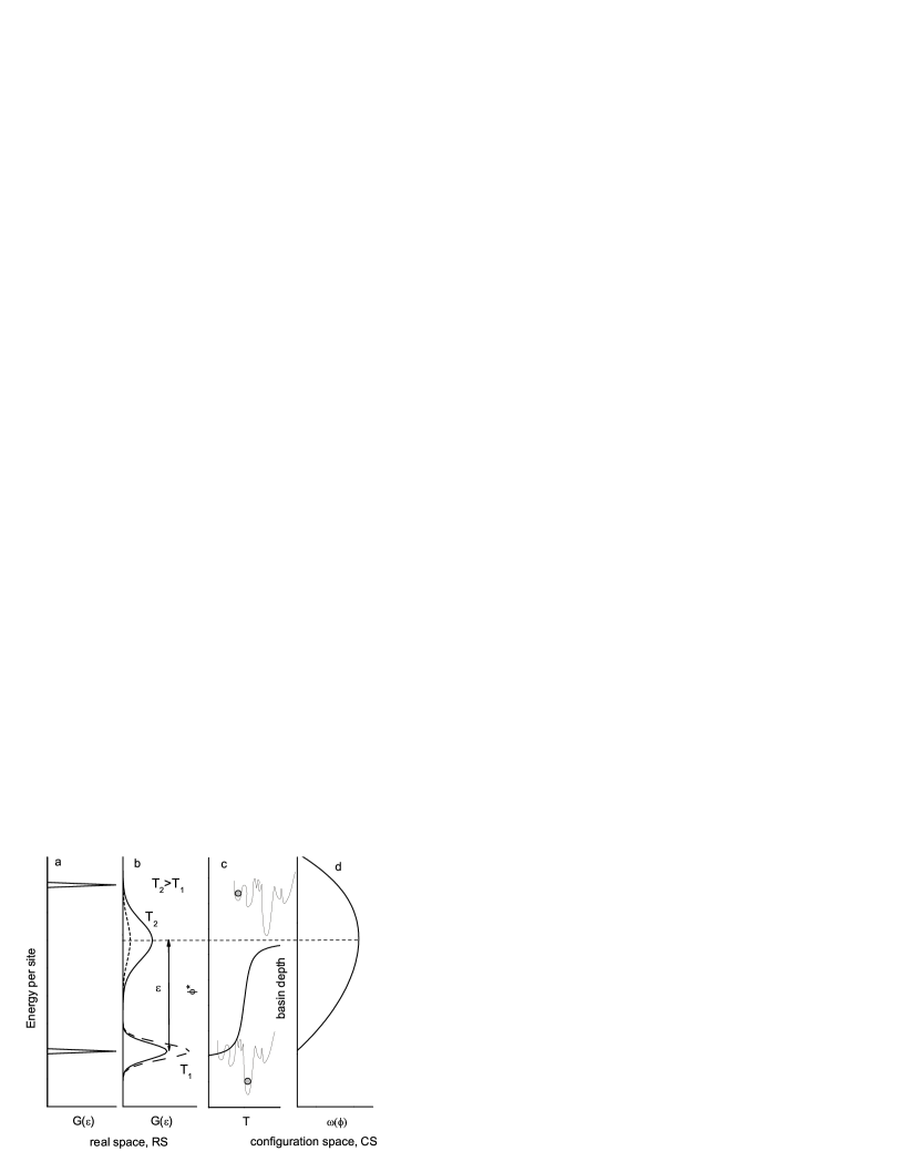
Figure 1: Real space (RS) energies of perfect crystal sites and defect sites (a). Real space energies and populations of the ideal glass and liquid sites at temperatures $T_{1}=T_{g}$ and $T_{2}$ respectively (b). Configuration space (CS) location of system points at $T_{1}=T_{K}$ and $T_{2}$, and the excitation profile (sigmoid) (c). Quasi-Gaussian enumeration function for configurational states (d).

In the present paper we show how thermodynamic behavior of the sort obtained on soft sphere mixturesGrigera and Parisi (2001); Yu and Carruzzo ; Yu and Carruzzo (2004); Yan et al. (2004) can be reproduced by a modified version of the simple excitations model in which the single (or few) excitation energy(ies) of the original models is(are) replaced by a more physically reasonable Gaussian distribution, the centroid of which may lie near but generally below the value of the original excitation energy, and the width of which may vary. The existence of such character has been suggested by analysis of spectral band-shapes for glasses and liquidsAngell (1980) and recently, also, the vibrational density of states of glasses of different fictive temperatures in which a quasi-two state behavior is found for the temperature dependence of the vibrational density of states.Mossa et al. (2002); Angell et al. (2003) We note that the Gaussian analysis that is often used to describe the widths of spectral bands, is only appropriate if the modes are localized - which is a poor approximation when dealing with the vibrational density of states, even for the boson peak.Gurevich et al. (2003) Other spectroscopic evidence for distinct broken bond excitations in glasses has been given for weak network liquidsAngell and Wong (1970) and recentlyAngell (2004); com (a) revived in connection with the boson peak controversy.

II Model representations in real space and configuration space (energy landscape).

The model assumes the presence in the condensed phase of degrees of freedom which, in real space (RS), can exist in ground (low-energy) and excited (high-energy) states.Angell and Rao (1972) To visualize the model and its relation to crystal defect physics on the one hand, and to energy landscape representations on the other, we use Fig. 1. The distribution of energies in the real space ground state, in the case of the crystal, is a delta function, on the unit cell length scale, and a small number of delta functions on the per molecule scale (Fig. 1a). The defect states are likewise few in number and well defined in energy. In the glass, however, the sites are not all equivalent on these length scales, and a Gaussian distribution in energy is expected, both for molecules in the ideal glass and for the elementary configurational excitation (or defect) states which we suppose to exist (Fig. 1b). Excitations may be related to coordination defects in covalent materials or to local distortions or packing strains in molecular crystals.

The distribution of energies $\epsilon_{i}$ in real space is characterized by two Gaussians $G_{i}(\epsilon_{i})$ where $i=1$ stands for the ground state and $i=2$ stands for the excited state. The Gaussian function $G_{i}(\epsilon_{i})$ is defined by the average $\epsilon_{0i}$ and the variance $\sigma_{i}$. In addition to the change in energy, the creation of a local defect may result in an entropy increase related either to a change in the vibrational or configurational density of states.Angell (2000) The entropy change per molecule of the glass is $s_{0}=\Delta S_{0}/Nk_{\text{B}}$.

The potential energy in configuration space (CS) is a hypersurface depending on all degrees of freedom of the disordered liquid. The overall configuration space is decomposed into basins of local potential energy minima termed inherent structures.Stillinger and Weber (1982); Stillinger (1988) The ideal glass, in configuration space, is represented by the lowest energy basin on the energy landscape, and any excitation of defect states will lift the energy to one or other of the higher energy basins. The more defects in the real space quasilattice, the higher the energy of the configuration space basin occupied by the system (Fig. 1c). Thus as the intensity or occupation number of the second real space Gaussian increases (cf. dashed to solid lines in Fig. 1b), the system point in configuration space moves higher on the landscape (Fig. 1c).

The distribution of basin energies (CS) is found, by simulation studies, to conform to a Gaussian (Fig. 1d), but it is barely possible to distinguish between a Gaussian and the binomial distribution that is expected for a two-state system, except at the wings, which are unexplored in any simulations on accessible time scales. The difference must diminish further for the case where the excitation energy is distributed, as in our model. Where a given excitation can occur at any energy in the real space distribution, the states in the configuration space distribution are only occupied on the low energy side of the maximum of the Gaussian (Fig. 1d). The energies in this half Gaussian, though, are uniformly higher than those in the crystal manifold, which is very narrow (Fig. 1c), because the crystal generates very few defects before it becomes thermodynamically unstable and melts.

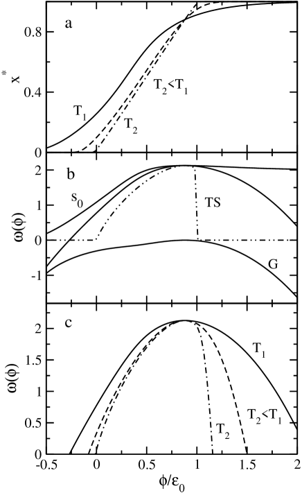
Figure 2: (a): $x^{*}=x(\phi^{*})$ calculates as the root of Eq. (21). (b) $\omega(\phi)$ from Eq. (10) and its separation into the ideal mixture term “$s_{0}$” (first summand in Eq. (10)) and the Gaussian term “G” (second summand in Eq. (10)). (c): $\omega(\phi)$ from Eq. (10). The lines in (a)–(c) refer to different temperatures: $T=500$ K (solid line), $T=200$ K (dashed line), and $T=10$ K (dash-dotted line); $\lambda_{2}/k_{\text{B}}=200$ K, $\lambda_{1}/k_{\text{B}}=100$ K, $\epsilon_{0}/k_{\text{B}}=800$ K, $s_{0}=2.0$. The dash-dotted line in (b) shows the enumeration function of the two-state, “TS”, model [Eq. (13)].

The density of inherent structures identified with basins of depth $\phi$ defines the enumeration function $\omega(\phi)$. Following DerridaDerrida (1980) and Wolynes,Bryngelson and Wolynes (1987) $\omega(\phi)$ can be found by summation over all populations of the excited state

$$e^{N\omega(\phi)}=\sum_{N_{2}=0}^{N}C(x)\left[P(\phi,x)\right]^{N},$$ (1)

where $N_{2}$ is the number of excitations out of $N$ molecules in the system, $x=N_{2}/N$ is the population of the excited state. The function $C(x)$ in Eq. (1) is the number of realizations of a given distribution of molecules between the ground and excited states

$$C(x)=\frac{N!}{(N-N_{2})!N_{2}!}e^{s_{0}N_{2}}.$$ (2)

The distribution of basin energies $P(\phi,x)$ in configuration space [Eq. (1)] can be obtained from the real space Gaussians (Fig. 1b),

$$P(\phi,x)=\int\delta\left(\phi-x\epsilon_{2}-(1-x)\epsilon_{1}\right)G_{2}(\epsilon_{2})G_{1}(\epsilon_{1})d\epsilon_{2}d\epsilon_{1}.$$ (3)

Equation (3) gives a Gaussian distribution of basin energies with the average and variance dependent on the population of excited states in real space

$$P(\phi,x)=\left[2\pi\sigma\right]^{-1/2}\exp\left[-\frac{(\phi-x\epsilon_{0})^{2}}{2\sigma(x)^{2}}\right],$$ (4)

where $\epsilon_{0}=\epsilon_{02}-\epsilon_{01}$ is the excitation energy and

$$\sigma(x)^{2}=(1-x)^{2}\sigma_{1}^{2}+x^{2}\sigma_{2}^{2}$$ (5)

is the variance of basin energies.

In the thermodynamic limit $N\to\infty$, the behavior of the sum in Eq. (1) is defined by its largest summand. One finds

$$\omega(\phi)=s(\phi,x(\phi)),$$ (6)

where the population at maximum $x(\phi)$ is obtained from the stationary point

$$\frac{ds(\phi,x)}{dx}\bigg{|}_{x=x(\phi)}=0.$$ (7)

The function $s(\phi,x)=S(\phi,x)/Nk_{\text{B}}$ is the entropy per molecule at a given population of excited states. From Eqs. (1), (2), and (4) one finds

$$s(\phi,x)=s_{0}(x)-\frac{(\phi-x\epsilon_{0})^{2}}{2\sigma(x)^{2}},$$ (8)

where $s_{0}(x)$ is the entropy of an ideal binary mixture

$$s_{0}(x)=xs_{0}-x\ln x-(1-x)\ln(1-x).$$ (9)

The requirement to maximize the entropy at a given basin depth makes the population $x$ a function of $\phi$ and, therefore, transforms the enumeration function

$$\omega(\phi)=s_{0}(x(\phi))-\frac{(\phi-x(\phi)\epsilon_{0})^{2}}{2\sigma(x(\phi))^{2}}$$ (10)

into a generally non-Gaussian dependence on $\phi$ (Fig. 2). The solution $x(\phi)$ is a root of Eqs. (7) and (8) (Fig. 2a).

In the static energy landscape picture a system at constant volume has a unique energy landscape in the configuration space that is fixed by the intermolecular potential for the particles in the system. From this viewpoint, it seems natural to assume that the variance $\sigma$ is independent of temperature. If, in addition, the dependence of $x(\phi)$ and $\sigma(\phi)$ on $\phi$ is neglected in Eq. (10), one arrives at the standard Gaussian model equivalent to the random energy model introduced by Derrida.Derrida (1980, 1981) The Derrida model predicts an ideal glass transition at the Kauzmann temperature $k_{\text{B}}T_{K}=\sigma/\sqrt{2s_{0}(x(\phi^{*}))}$ ($\omega(\phi^{*})=0$ at $T=T_{K}$) and a hyperbolic temperature dependence of the average basin energy

$$\phi^{*}=a-b/T.$$ (11)

The dependence of the type given by Eq. (11) has indeed been observed in several simulation studies of binary Lennard-Jones (LJ) mixtures,Sastry (2001); Mossa et al. (2002) although deviations from this law have also been reported.Büchner and Heuer (1999); Heuer and Büchner (2000); Saika-Voivod et al. (2001, 2004); Saksaengwijit et al. (2004) The heat capacity per molecule $c_{V}=C_{V}/Nk_{\text{B}}=k_{\text{B}}^{-1}d\phi^{*}/dT$ then varies as $c_{V}\propto 1/T^{2}$.

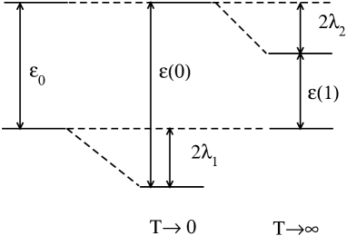
Figure 3: Temperature dependence of the effective excitation energy $\epsilon(x^{*})$ [Eq. (22)]. $\epsilon(0)$ and $\epsilon(1)$ denote the excitation energy at zero and infinite temperature, respectively.

In the limit when the RS Gaussians are much narrower than the excitation energy, $\sigma_{i}\ll\epsilon_{0}$, one gets the two-state model.Angell and Rao (1972) The Gaussian term in Eq. (10) then generates a delta function in the density of states $e^{\omega(\phi)}$ requiring $x(\phi)=\phi/\epsilon_{0}$. This solution also limits the range of accessible basin depths by the condition

$$0\leq\phi\leq\epsilon_{0}.$$ (12)

The enumeration function in this limit corresponds to the logarithmic energy landscape of Debenedetti, Stillinger, and ShellDebenedetti et al. (2003)

$$\omega^{\text{TS}}(\phi)=s_{0}u-u\ln(u)-(1-u)\ln(1-u),$$ (13)

where $u=\phi/\epsilon_{0}$, $0\leq u\leq 1$ and the superscript “TS” refers to the two-state model. Note that $s_{0}=0$ is used in the logarithmic model in Ref. Debenedetti et al., 2003.

The average basin depth is proportional to the population $x_{\text{TS}}^{*}$ of the RS excited states in the two-state limit:

$$\phi^{*}=x_{\text{TS}}^{*}\epsilon_{0},\quad x_{\text{TS}}^{*}=[1+e^{-s_{0}+\beta\epsilon_{0}}]^{-1},$$ (14)

$\beta=1/k_{\text{B}}T$. The constant volume heat capacity per particle (in $k_{\text{B}}$ units) is of Schottky’s formMoynihan and Angell (2000); Odagaki et al. (2002)

$$c_{V}^{\text{TS}}=(\beta\epsilon_{0})^{2}x_{\text{TS}}^{*}(1-x_{\text{TS}}^{*}).$$ (15)

This heat capacity form is continuous down to zero K hence, as is well known,Angell and Rao (1972); Perez (1985); Angell (2000); Moynihan and Angell (2000) the two-state model eliminates the ideal glass transition ($T_{K}\to 0$). Thus variation of the Gaussian width parameters of our model produces the same systematic change of heat capacity form that Debenedetti et al.Debenedetti et al. (2003) demonstrated by ad hoc linear mixing of the Gaussian and binomial distribution CS functions. The heat capacity function for laboratory glasses of different fragility should then reflect the width of the RS Gaussians relative to the separation of their centers.

The present model, which we will refer to as the two-Gaussian (2G) model, projects the two RS Gaussians onto CS enumeration function given by Eq. (10). $\omega(\phi)$ in Eq. (10) is formally a linear combination of the ideal mixture entropy of the RS two-state model and the CS Gaussian term of the Gaussian model. The two terms are connected through the $x(\phi)$ function. $x(\phi)$ is not a linear function of the two-state model [Eq. (14)] when $\sigma_{i}\neq 0$, although it approaches the linear limit with lowering temperature (Fig. 2a) when RS Gaussians become narrower (see Eq. (20)).

Both the ideal mixture term $s_{0}(x)$ (first summand in Eq. (10)) and the Gaussian term (second summand in Eq. (10)) are non-parabolic functions of $\phi$. A bell-shaped enumeration function, which at high temperatures can be approximated by a Gaussian shape, is a result of combining two non-Gaussian summands in Eq. (10) (Fig. 2b). The two-state limit of the 2G model results in a very asymmetric enumeration function when the excitation entropy $s_{0}$ is non-zero due to the cutoff of the range of accessible basin energies (Eq. (12); dash-dotted line in Fig. 2b).

The connection between the microcanonical entropy $\omega(\phi)$ and the canonical ensemble, which permits calculations at given temperatures, can be obtained by use of two thermodynamic relationsLandau and Lifshits (1980)

$$\left(\frac{\partial\omega(\phi)}{\partial\phi}\right)_{N,V}=\beta$$ (16)

and

$$\left(\frac{\partial^{2}\omega(\phi)}{\partial\phi^{2}}\right)_{N,V}=-\frac{\beta^{2}}{c_{V}}.$$ (17)

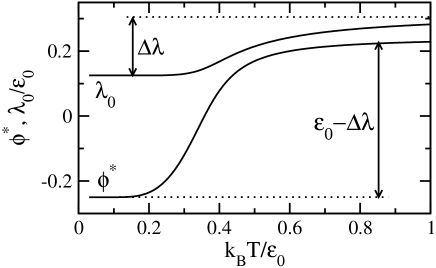
Figure 4: $\lambda_{0}(T)$ [Eq. (19)] and $\phi^{*}$ [Eqs. (18) and (21)] vs temperature; $\lambda_{1}/k_{\text{B}}=100$ K, $\lambda_{2}/k_{\text{B}}=200$ K, $\epsilon_{0}/k_{\text{B}}=800$ K, $s_{0}=2.0$.

Equation (16) leads to the average energy of inherent structures

$$\phi^{*}=x^{*}\epsilon_{0}-2\lambda_{0},$$ (18)

where $x^{*}=x(\phi^{*})$ and

$$\lambda_{0}=(1-x^{*})^{2}\lambda_{1}+(x^{*})^{2}\lambda_{2}.$$ (19)

The coupling parameters $\lambda_{i}$ in Eq. (19) are defined in terms of the RS distribution widths as

$$\sigma_{i}^{2}=2k_{\text{B}}T\lambda_{i}.$$ (20)

Equations (5) and (19) immediately lead to Eq. (14) in the limit of narrow RS Gaussians, $\lambda_{i}\to 0$. Once Eq. (18) is substituted into Eq. (7), one arrives at a single, self-consistent equation for $x^{*}$ which is used to obtain the average energy $\phi^{*}$ in Eq. (18):

$$x^{*}=\left[1+e^{-s_{0}+\beta\epsilon(x^{*})}\right]^{-1}.$$ (21)

Here, $\epsilon(x^{*})$ is the population-dependent average excitation energy

$$\epsilon(x^{*})=\epsilon_{0}-2x^{*}\lambda_{2}+2(1-x^{*})\lambda_{1}.$$ (22)

Mechanical stability of the ideal glass state requires

$$\epsilon(x^{*})>0.$$ (23)

Equation (21) indicates that the introduction of finite widths to the two RS delta functions of the two-state model results in self-consistency in determining the excited-state population which is governed by the average ground-to-excited energy gap $\epsilon(x)$ [cf. Eqs. (14) and (21)]. The function $\epsilon(x)$ has a simple physical meaning. Going from two states with the gap $\epsilon_{0}$ to a disordered material with Gaussian distributions of the RS ground and excited state energies makes states with lower random energies thermodynamically more probable. This effectively lowers the energy of each RS state by “solvation” energy $2\lambda_{i}$ (Stokes shift in spectroscopic applications). The lowering of the energy of each state is, however, scaled with the corresponding population and one gets $2x\lambda_{2}$ and $2(1-x)\lambda_{1}$ for lowering the excited and ground states, respectively. The dependence on ground and excited state populations makes the excitation energy decrease with increasing temperature from $\epsilon_{0}+2\lambda_{1}$ at low temperature to $\epsilon_{0}-2\lambda_{2}$ at high temperature (Fig. 3).

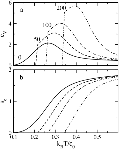
Figure 5: $c_{V}$ (a) and $s_{c}$ (b) (in $k_{\text{B}}$ units) vs temperature at $\lambda_{1}=0$ (solid line), $\lambda_{1}/k_{\text{B}}=50$ K (dashed line), $\lambda_{1}/k_{\text{B}}=100$ K (dash-dotted line), and $\lambda_{1}/k_{\text{B}}=200$ K (dash-double-dotted line); $\lambda_{2}/k_{\text{B}}=200$ K, $\epsilon_{0}/k_{\text{B}}=800$ K, $s_{0}=2.0$, $\lambda_{1}$ and $\lambda_{2}$ are assumed to be temperature independent. Numbers on plot (a) indicate values of $\lambda_{1}/k_{\text{B}}$.

The second thermodynamic relation [Eq. (17)] allows one to connect the width parameter $\sigma$ in the CS Gaussian term in Eq. (10) and the constant-volume heat capacity per molecule $c_{V}(T)$. The width in the Gaussian term can be separated into the $k_{\text{B}}T$ factor and an energetic coupling parameter related to the RS coupling constants $\lambda_{i}$ [Eqs. (19) and (20)]:

$$\sigma^{2}=2k_{\text{B}}T\lambda_{0}(T),$$ (24)

The form of the CS Gaussian width in Eq. (24) is dictated by the classical limit of the fluctuation-dissipation theorem (FDT).Landau and Lifshits (1980) The energy parameter $\lambda_{0}(T)$ then plays the role of the trapping energy in theories of random-media conductivityBässler (1987) or the solvent reorganization energy in theories of electron transfer.Marcus (1993) Alternatively, $\lambda_{0}(T)$ enters the constant volume heat capacity obtained from Eqs. (10) and (17)

$$c_{V}(T)=2\beta\lambda_{0}(T)\left[1-\alpha^{*}(\epsilon_{0}-4x^{*}\lambda_{2}+4(1-x^{*})\lambda_{1})\right]^{-1},$$ (25)

where

$$\alpha^{*}=\frac{dx(\phi)}{d\phi}\bigg{|}_{\phi=\phi^{*}}.$$ (26)

The separation of the width $\sigma^{2}$ in the $k_{\text{B}}T$ factor and $\lambda_{0}(T)$ is convenient when the latter is only weakly dependent on temperature. This implies that $c_{V}(T)$ is approximately a hyperbolic function of temperature $c_{V}(T)\propto 1/T$ as is empirically documented, at least for the constant pressure heat capacity.Privalko (1980); Aba et al. (1990) The temperature dependence of $\lambda_{0}(T)$ [Eq. (19)] is determined by the gap $\Delta\lambda=\lambda_{2}-\lambda_{1}$ in the coupling parameters between the ground and excited states since $\lambda_{0}(T)$ has a sigmoidal form (Fig. 4) with the change $\Delta\lambda$ from low to high temperatures ($\lambda_{i}$ are assumed to be temperature independent in Fig. 4). A qualitatively similar sigmoidal form often observed in simulationsSastry et al. (1998); Jung et al. (2004); Doliwa and Heuer (2003); Chowdhary and Keyes (2004) is seen for the basin depth $\phi^{*}$. The basin depth increases by the amount $\epsilon_{0}-2\Delta\lambda$ with increasing temperature (Fig. 4).

The description of the glass thermodynamics in terms of a distribution of basin energies involves the projection of the whole configuration space onto a single collective coordinate. This projection onto the lower dimensionFeynman and F. L. Vernon (1963) introduces a reduced description of the system thermodynamics reflected by the temperature dependence of the moments of the collective coordinate, as is well known from e.g. electron transfer theory.Marcus (1993) In fact, thermodynamics [Eq. (17)] and the classical limit of the FDT [Eq. (24)] both predict that, for fluctuations caused by classical motions, $\sigma^{2}$ should decompose into the $k_{\text{B}}T$ factor and a coupling parameter $\lambda_{0}(T)$. This is a significant departure from the simple temperature independent behavior of $\sigma^{2}$ supposed to date. Such a temperature dependence modifies predictions of even the simple Gaussian model: no ideal glass transition occurs for temperatures which leave the expression $s_{0}(x^{*})-\beta\lambda_{0}(T)$ positive. We also note that the combination of disorder with the FDT leads to the excitation energy $\epsilon(x^{*})$ [Eq. (22)] decreasing with temperature.

The distribution of basin energies is affected by temperature through the explicit $k_{\text{B}}T$ factor in Eq. (24) and through a more complex temperature variation of $\lambda_{0}(T)$. Figure 2c shows $\omega(\phi)$ at different temperatures obtained under the assumption that $\lambda_{i}$ defined by Eq. (20) are temperature independent. The distribution, which is almost Gaussian at high temperatures, gets skewed from the high-energy wing at lower temperatures (cf. solid and dash-dotted lines in Fig. 2c). The low-energy wing of the enumeration function is not strongly affected by temperature, and low-energy wings at different temperatures can approximately be brought to one master curve by a vertical shift. The high-energy wings differ, however, substantially as temperature changes. Exactly this behavior of the enumeration function curves at different temperatures is reported for the 80-20 LJ binary mixture in Fig. 4 of Ref. Sciortino et al., 2000.

The enumeration function taken at the average basin depth $\phi^{*}$ gives the configurational entropy (in $k_{\text{B}}$ units)

$$s_{c}=s_{0}(x^{*})-\beta\lambda_{0}.$$ (27)

This equation predicts the existence of ideal glass transition, $s_{c}(T_{K})=0$, at a finite temperature when $\lambda_{1}\neq 0$. The Kauzmann temperature $T_{K}$ tends to zero when $\lambda_{1}\to 0$ and $s_{c}>0$ for any $0<x^{*}<1$ at $\lambda_{1}=0$ (solid line in Fig. 5b). The constant volume heat capacity can directly be calculated from Eq. (25). Calculations of $c_{V}(T)$ at constant $\lambda_{2}$ and varying $\lambda_{1}$, both temperature independent, are shown in Fig. 5a. At $\lambda_{1}\neq 0$ the heat capacity drops to zero at the point of ideal glass transition at $T=T_{K}>0$. There is no ideal glass transition when $\lambda_{1}=0$, and the heat capacity passes through a broad maximum.

Table 1: Best-fit parameters for model fluids (rows 1-2) and real liquids (rows 3-6). For real liquids, the fitting parameters are $\lambda_{1}$, $\lambda_{2}$, $\epsilon_{0}$ (K) and $s_{0}$ are obtained by global fits of Eqs. (22) and (32) to experimental heat capacities and entropies.

Substance	$z$	$T_{g}$	$T_{\text{fus}}$	$\Delta s_{\text{fus}}$	$\epsilon_{0}/k_{\text{B}}$	$\lambda_{1}/k_{\text{B}}$	$\lambda_{2}/k_{\text{B}}$	$s_{0}$	$T_{K}$	$T_{K}$
80-20 BLJM	1				69.3	8.9	26.5	0.14	34.35	30.4
50-50 BSSM	1				78.5	2.0	22.3	1.59		14.2
Glycerol	8	190	291	7.55	631	18	32	1.27	136.7	130
Selenium	1	304	494.33	1.50	905	14	27	1.7	210.7	153
Toluene	2	117	178.15	4.48	1045	36	518	5.1	99.9	110
$o$-terphenyl	2	246	329.4	6.28	2267	45	1133	5.5	204.1	214

III Liquid-Liquid(Glass) First Order Phase Transition

Depending on the value of the excitation entropy $s_{0}$ Eq. (21) may have one, two, or three solutions. Only one solution exists for low $s_{0}$ since the condition of mechanical stability requires that the effective excitation energy $\epsilon(x^{*})$ remains positive at all excited state populations [Eq. (23)]. Increasing the entropy of excitation allows one to reach the condition of vanishing Gibbs energy of excitation

$$g(x^{*})=\epsilon(x^{*})-k_{\text{B}}Ts_{0}$$ (28)

in the range $0\leq x^{*}\leq 1$. At the temperature

$$T_{LL}=(\epsilon_{0}-\Delta\lambda)/s_{0}$$ (29)

the excitation Gibbs energy vanishes at $x^{*}=1/2$, $g(1/2)=0$. This is the temperature of the equilibrium liquid-liquid, first-order phase transition between the low-temperature liquid with low concentration of excitations and the high-temperature liquid with high concentration of excitations.Sastry and Angell (2003); Tanaka et al. (2004) This transition becomes a liquid-glass transition when the low-temperature phase has its viscosity below the glass transition limit or when the transition occurs directly to the ideal glass state.

The first order transition is possible for temperatures below the critical temperature $T_{c}$ and excitation entropies above the critical value $s_{0c}$:

$$T<T_{c},\quad s_{0}>s_{0c}.$$ (30)

The critical parameters are

$$\begin{split}k_{\text{B}}T_{c}&=\bar{\lambda}=(\lambda_{1}+\lambda_{2})/2,\\ s_{0c}&=\frac{\epsilon_{0}-\Delta\lambda}{\bar{\lambda}}.\end{split}$$ (31)

The critical temperature $T_{c}$ increases and the critical entropy $s_{0c}$ decreases with enhanced disorder of the excited state (Fig. 6). When $T<T_{c}$ and $s_{0}>s_{0c}$, the equilibrium transition temperature, $T_{LL}$, is flanked by lower, $T_{l}$, and upper, $T_{u}$, spinodal temperatures at which only two solutions of Eq. (21) are possible: $T_{l}\leq T_{LL}\leq T_{u}$ (Fig. 6).

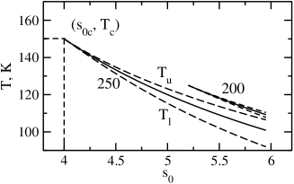
Figure 6: Equilibrium first-order transition temperature (solid lines) and the lower, $T_{l}$, and upper, $T_{u}$, spinodal temperatures (dashed lines) vs the excitation entropy $s_{0}$. The calculations are carried out for $\epsilon_{0}/k_{\text{B}}=800$ K, $\lambda_{1}=50$ K, and values of $\lambda_{2}/k_{\text{B}}$ indicated on the plot; $(s_{0c},T_{c})$ indicates the critical point.

Figure 7 illustrates the change in the temperature variation of the thermodynamic parameters with increasing the excitation entropy $s_{0}$. At $s_{0}<s_{0c}$, the entropy and basin energy are both continuous functions of temperature. The heat capacity passes through a broad maximum characteristic of the two-state model and drops to zero at a Kauzmann temperature $T_{K}>0$ when $\lambda_{1}\neq 0$. At the critical excitation entropy $s_{0}=s_{0c}$, the entropy and energy both pass through an inflection point reflected by a lambda singularity in the constant volume heat capacity. Finally, the liquid-liquid (glass) phase transition occurs above $s_{0c}$. The entropy drop at the transition temperature increases with increasing $s_{0}$ to the point where the entropy drops to zero. This transition, as well as all transitions with higher entropy $s_{0}$, occur directly from the supercooled liquid to the ideal glass state.

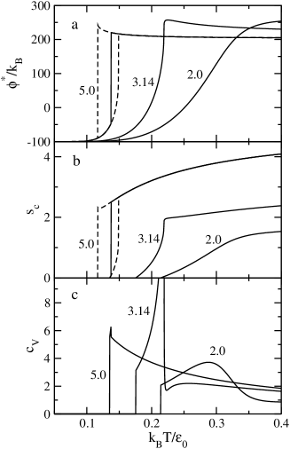
Figure 7: Basin energy (a), configuration entropy (b), and constant-volume heat capacity (c) at the values of $s_{0}$ indicated on the plot; $\lambda_{1}/k_{\text{B}}=50$ K, $\lambda_{2}/k_{\text{B}}=300$ K, $\epsilon_{0}/k_{\text{B}}=800$ K. The values $s_{0}=3.14$ and $k_{\text{B}}T/\epsilon_{0}=0.22$ correspond to the critical point at which lambda singularity for the heat capacity is seen. The dashed lines indicate metastable states between the lower and upper spinodal temperatures.

IV Comparison to simulations

The temperature variation of the energy landscape is critically affected by the approximately linear temperature dependence of the width parameter $\sigma$ [Eq. (24)] which contributes to the overall temperature variation of the distribution of basin energies

$$P(\phi)\propto e^{\omega(\phi)-\beta\phi}.$$ (32)

This generally non-Gaussian distribution is often approximated by a Gaussian function:

$$P(\phi)\propto\exp\left(-\frac{(\phi-\phi^{*})^{2}}{2\Gamma^{2}}\right)$$ (33)

with the empirical Gaussian width $\Gamma$. Computer simulations of $P(\phi)$ and the constant volume heat capacity $c_{V}$ at varying temperature may provide insights into the temperature dependence of $\sigma$. Approximately Gaussian distribution of basin energies has been found in simulations of binary LJSpeedy and Debenedetti (1988); Büchner and Heuer (1999); Sciortino et al. (2000); Sastry (2001) and hard sphere fluids.Speedy and Debenedetti (1988) Although an increase of the width with temperature is often seen in simulations,Sastry et al. (1998); Sciortino et al. (2000) numerical data are very limited.

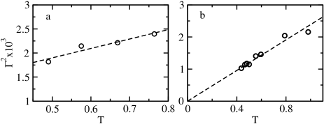
Figure 8: Variance of the distribution of metabasins in the A-B binary LJ fluid determined from simulations by Denny et alDenny et al. (2003); com (b) (a) and by Doliwa and HeuerDoliwa and Heuer (2003) (b). Units of energy and temperature are defined by the LJ energy of the A-A interaction potential.

Temperature-dependent width $\Gamma(T)$ can be found in simulations of the well-known 80-20 LJ mixtureWeber and Stillinger (1985); Kob and Andersen (1995) by Büchner and Heuer.Büchner and Heuer (1999); Heuer and Büchner (2000) Also, recent extensive simulations by Denny et al.Denny et al. (2003) and by Doliwa and HeuerDoliwa and Heuer (2003) give the variance of energies of metabasins (basins separated by small minima which do not require activated hops at a given temperatureStillinger (1995); Doliwa and Heuer (2003)) for the same system at different temperatures. The width of metabasin distribution $\Gamma(T)$ extractedcom (b) from the simulations by Denny et al.Denny et al. (2003) is approximately linear in $T$ (Fig. 8a). An even steeper $\Gamma(T)$ is found in simulations by Doliwa and HeuerDoliwa and Heuer (2003) of the same system of a smaller size (Fig. 8b).

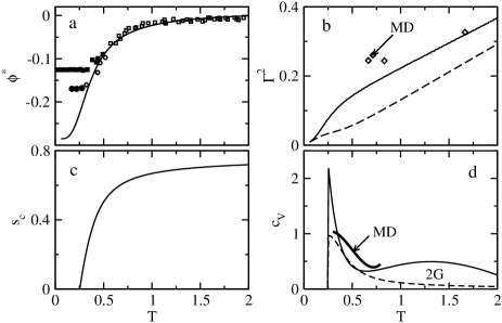
Figure 9: Inherent structure energy (a), the distribution width (b), configurational entropy (c), and constant volume heat capacity (d) for the 80-20 LJ binary mixture.Kob and Andersen (1995); Sastry et al. (1998); Sastry (2001) The solid lines refer to calculations with the present model with the parameters obtained from the fit of inherent structure energies from Ref. Sastry et al., 1998 combining data for the cooling rate 2.7 $\texttimes 10^{-4}$ (squares) and 3.33$\texttimes 10^{-6}$ (circles). The closed points in (a) indicate the points which were excluded from the fit since they represent the loss of system’s ergodicity due to finite cooling rate. In (b), the solid line refers to $\Gamma^{2}$, the dashed line refers to $\sigma^{2}$, and “MD” refers to simulation results for $\Gamma^{2}$ by Büchner and Heuer.Büchner and Heuer (1999); Heuer and Büchner (2000) In (d), the dashed line refers to the constant $P$ heat capacity calculated under assumption that $\lambda_{i}$ are temperature independent. The bold solid line marked “MD” is obtained by numerical differentiation of the configurational entropy from MD simulations by Sciortino et al.Sciortino et al. (1999) and “2G” marks the present model. Units of energy and temperature are defined by the LJ energy of the A-A interaction potential. The parameters of the fit are listed in Table 1.

The 2G model is based on four parameters: $\epsilon_{0}$, $\lambda_{1}$, $\lambda_{2}$, and $s_{0}$. The model is tested on its ability to reproduce several thermodynamic observables for a single set of parameters. We first apply the 2G model to simulations of model fluids and then, in Sec. V, apply it to real liquids. For comparison to computer experiment we fit the average basin energy from 2G model to combined ergodic parts of two cooling runs reported in Ref. Sastry et al., 1998 for the 80-20 binary LJ mixture (Fig. 9a, Table 1). The fitting parameters obtained for the basin depth are used to calculate the configurational entropy [Eq. (27)] which goes to zero (Fig. 9c) at the Kauzmann temperature very close to that obtained from simulations of $s_{c}$ itself and to $T_{0}$ from diffusivity extrapolated to zero through the Vogel-Fulcher-Tammann plot (cf. columns 10 and 11 in Table 1).

Since the distribution $P(\phi)$ is generally non-Gaussian, the empirical width $\Gamma$ was obtained from the half-intensity width of $P(\phi)$. $\Gamma^{2}$ (solid line in Fig. 9b) is larger than $\sigma^{2}$ (dashed line in Fig. 9) since the former reflects the overall width arising from the ideal mixture entropy and the CS Gaussian term in Eq. (10) combined. The empirical width $\Gamma^{2}(T)$ rises with temperature in accord with the prediction of the FDT and the results of simulations. The magnitude of $\Gamma^{2}$ for the distribution of basins is significantly larger than the one for the distribution of metabasins (cf. Fig. 8 and Fig. 9b). However, the variance of basin energies from MD simulations by Büchner and HeuerBüchner and Heuer (1999); Heuer and Büchner (2000) (marked “MD” in Fig. 9b) is in reasonable agreement with the 2G model. Finally, the constant volume heat capacity shows a steep rise on approach to the ideal glass transition, dropping to zero at $T_{K}$. This form of the heat capacity is supported by simulations of Sciortino et al.Sciortino et al. (1999) as shown in Fig. 9d. We note that the 80-20 system was originally parameterized to represent the metallic Ni-P alloyWeber and Stillinger (1985) and that metallic glassformers typically show very sharp excess heat capacity functions relative to molecular and ionic glassformers.Angell (1995); Busch (2000)

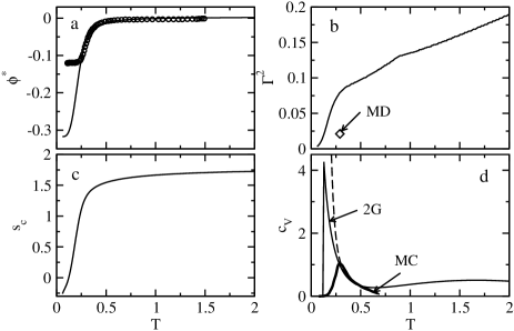
Figure 10: Same as in Fig. 9 for the 50-50 BSSM studied by Yan et al.Yan et al. (2004). The parameters of the fit are listed in Table 1. In (b), “MD” marks the Gaussian width from parallel tempering MD simulations reported in Refs. Yu and Carruzzo, and Yu and Carruzzo, 2004. In (d), “2G” marks the present two-Gaussian model, the bold line marked “MC” refers to the results of Monte Carlo simulations from Ref. Yan et al., 2004. The dashed line shows the fit of the $c_{V}$ simulation dataYu and Carruzzo (2004) extrapolated below the temperature of heat capacity drop. The functional form of $c_{V}(T)$ (dashed line) is from Ref. Yu and Carruzzo, 2004: $c_{V}(T)=A_{1}T^{B_{1}}+A_{2}T^{B_{2}}$, $A_{1}=2.845$, $B_{1}=-0.209$, $A_{2}=3.477\texttimes 10^{-4}$, $B_{2}=-5.804$.

A similar fit of the 2G model to the average basin depth of the 50:50 soft sphere (SS) mixture reported by Yan et al.Yan et al. (2004) is shown in Fig. 10. The parameters of the fit are used to calculate the distribution width $\Gamma$ (Eq. (33), Fig. 10b), the configurational entropy (Eq. (27), Fig. 10c), and the constant volume heat capacity (Eq. (25), Fig. 10d). The basin energy width calculated from 2G model ($\Gamma/\epsilon_{AA}=0.08$) is higher than the one observed in simulationsYu and Carruzzo ; Yu and Carruzzo (2004) ($\Gamma/\epsilon_{AA}=0.02$, marked “MD” in Fig. 10b).

Despite the use of parallel tempering MD in Refs. Yu and Carruzzo, and Yu and Carruzzo, 2004, the drop of the heat capacity at the peak temperature $T_{p}\simeq 36.5$ K ($\epsilon_{AA}/k_{\text{B}}=119.8$ K) seen in the simulations is due to insufficient sampling of the phase space.Yu and Carruzzo ; Yu and Carruzzo (2004) The parameters obtained from the fit of the average basin depth (Table 1) give a reasonable description of the simulated $c_{V}(T)$ up to $T_{p}$ followed by a much stronger rise of $c_{V}(T)$ which drops to zero at $T_{K}\simeq 14$ K. This latter temperature is close to the point of vanishing configurational heat capacity in the simulations. Note that a peak of $c_{V}(T)$ higher that the one reported in Refs. Yan et al., 2004, Yu and Carruzzo, , and Yu and Carruzzo, 2004 was obtained in MC simulations of analogous binary SS mixture by Grigera and ParisiGrigera and Parisi (2001) within a simulation protocol outperforming parallel tempering. This implies that, once sampling is improved, $c_{V}(T)$ continues to grow beyond the drop at $T_{p}$. Also note that extrapolation of $c_{V}(T)$ from the fit of simulation data by Yu and CarruzzoYu and Carruzzo (2004) to lower temperatures goes even steeper (dashed line in Fig. 10d) than $c_{V}(T)$ from 2G model.

V Experimental configurational entropies and the Kauzmann temperature

The configurational heat capacity of a liquid is normally taken as the difference between the liquid and crystal entropies reported for constant pressure, although it is known that in many cases a part of the entropy of fusion is due to an increase in the vibrational entropy (arising from increases in the low frequency vibrational density of states in the liquid inherent structuresGoldstein (1976); Angell (2004); Chowdhary and Keyes (2004)). The constant $P$ configurational heat capacity can be calculated from the configurational entropy in Eq. (27)

$$c_{P}=T\left(\frac{\partial s_{c}}{\partial T}\right)_{P}.$$ (34)

The unknown parameter in this calculation is the temperature dependence of the model parameters $\epsilon_{0}$, $\lambda_{i}$, and $s_{0}$ at constant $P$. Spectroscopic measurements at constant $P$ give “solvation energies” $\lambda_{i}$ through spectral Stokes shiftsRichert (2000) which are weakly temperature dependent.Vath et al. (1999) The Stokes shift relates to the coupling of a localized state to a thermal Gaussian bath. Since the defect excitations considered here may be more or less delocalized, it is currently unclear if the assumption $(\partial\lambda_{i}/\partial T)_{P}=0$ is warranted. An alternative scenario might include no temperature dependence of the ideal glass distribution $\sigma_{1}$ corresponding to quenched disorder (i.e., $\lambda_{1}\propto 1/T$) and a standard dependence on temperature of $\sigma_{2}$ (i.e., $\lambda_{2}=Const$). It turns out that, when the 2G model is applied to fit the experimental excess heat capacities of the liquid over the crystal, $\Delta c_{P}=c_{P,\text{liq}}-c_{P,\text{cryst}}$, the results are fairly insensitive to the assumptions made regarding the temperature dependence of $\lambda_{1}$ once the condition $\lambda_{2}(T)=Const$ is adopted. The fit of experimental results is thus done with temperature-independent $\epsilon_{0}$, $\lambda_{i}$, and $s_{0}$.

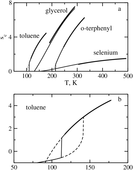
Figure 11: (a): Configurational entropy $s_{c}$ vs temperature for liquids listed in Table 1. Thick solid lines are experimental results and the thin solid lines are fits to the 2G model. Experimental data stop at the glass transition temperature $T_{g}$. Dotted lines show the extrapolation of experimental entropies to the zero entropy line. The fitting parameters are listed in Table 1. (b): Temperature dependence of the entropy of toluene (scaled up). The dashed lines indicate the entropies of metastable states terminated at the lower and upper spinodal temperatures.

The fitting procedure involves simultaneous fit of Eqs. (27) and (34) with four fitting parameters, ($\lambda_{1}$, $\lambda_{2}$, $\epsilon_{0}$, and $s_{0}$) to experimental heat capacities $\Delta c_{P}$ and experimental configurational entropies.Moynihan and Angell (2000) The range of energy parameters is restricted by the condition of mechanical stability of the ideal glass state [Eq. (23)]. The configurational entropy at constant $P$ can be determined experimentally from the entropy of fusion $\Delta s_{\text{fus}}$ and $\Delta c_{P}(T)$ (both in $k_{\text{B}}$ units)

$$s_{c}(T)=\Delta s_{\text{fus}}+\int_{T_{\text{fus}}}^{T}(\Delta c_{P}(T^{\prime})/T^{\prime})dT^{\prime}.$$ (35)

The 2G model outlined in Sec. II assumes that each molecule represents one excitable unit. While this is true for atomic glasses like selenium, for more complex compounds one needs to introduce the number $z$ of independently excitable (i.e. rearrangeable) states per molecule or formula unit.Moynihan and Angell (2000) The parameter $z$ is taken from Takeda et al.Takeda et al. (1999) (Table 1) and is used to multiply the heat capacity in Eq. (34) in fitting the experimental data. The results of the fit for four glassformers are listed in Table 1.

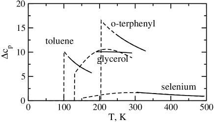
Figure 12: Comparison of the experimental values of $\Delta c_{P}$ (solid lines) with $\Delta c_{P}$ calculated from the 2G model (dashed lines) by simultaneous fit to the experimental $s_{c}$ and $\Delta c_{P}$ data above $T_{g}$.

The examination of Table 1 shows that $\lambda_{1}>0$ for all fluid studied, indicating that $T_{K}>0$. The distribution of excited states is much narrower in the case of covalent and hydrogen-bonded liquids (selenium and glycerol) compared to molecular liquids (toluene and $o$-terphenyl). In contrast, the RS distribution of the ideal glass is almost invariant among different glassformers. When $\lambda_{2}\gg\lambda_{1}$ the configurational entropy $s_{c}(T)$ gains a bend close to the Kauzmann point (Fig. 11) resulting in the actual $T_{K}$ from $s_{c}(T_{K})=0$ smaller than the corresponding value from extrapolation of experimental entropies (e.g., selenium in Table 1).

The most interesting result of our analysis is the low-temperature behavior of fragile molecular glasses (toluene and $o$-terphenyl). These substances are characterized by high disorder of the excited state ($\lambda_{2}\gg\lambda_{1}$, Fig. 13) and, in addition, high entropy of excitation (Table 1). It also turns out that $s_{0}$ from the fit is higher than the critical excitation entropy which is close to 2.0 for both liquids. The fact that $s_{0}$ is more than twice higher than $s_{0c}$ ensures low first-order transition temperature, well below the critical temperature (543 K for toluene and 1156 K for $o$-terphenyl). The first-order transition temperature in fact falls in the unobservable range between $T_{K}$ and $T_{g}$ where the entropy discontinuously drops to zero producing a similar drop in the heat capacity (Figs. 11 and 12). It may be therefore suggested that fragile liquids resolve the Kauzmann paradox by a first order liquid-glass transition. We note that both for toluene and $o$-terphenyl the lower spinodal temperature is below the point when metastable entropy crosses the zero entropy line while the upper spinodal temperature is above $T_{g}$ for toluene and almost coincides with $T_{g}$ for $o$-terphenyl. Since the first order transition is below $T_{g}$, the equilibrium passage along the solid line in Fig. 11b is unlikely thus suggesting hysteresis of the heat capacity between the cooling and heating runs.

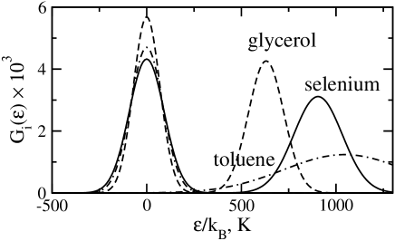
Figure 13: Real-space distribution of energies for selenium (solid lines), glycerol (dashed lines), and toluene (dash-dotted lines) at their corresponding Kauzmann temperatures. The parameters $\epsilon_{0}$ and $\lambda_{i}$ used in the calculations are taken from Table 1.

The value $s_{0}$, which remains an empirical parameter of the 2G model, can be compared to the entropy cost of creating a density wave in density-functional theories of aperiodic structures.Dasgupta and Valls (1999); Xia and Wolynes (2000) The average entropy of the “entropy droplet” in Wolynes’s mosaic model is

$$s_{0}=\frac{3}{2}\ln\left(\alpha r_{0}^{2}/\pi\right)-\frac{5}{2},$$ (36)

where $\alpha$ represents the rms displacement from the lattice site and $r_{0}$ is the mean lattice spacing. Invoking the Lindemann ratioXia and Wolynes (2000) $\alpha^{1/2}r_{0}=10$, one gets $s_{0}=2.7$, which falls in between entropies for strong and fragile liquids in Table 1.

Caution is needed in these interpretations since the model is in the early stages of evaluation and there are four parameters even for simply constituted glasses ($z=1$). One of these parameters may be disposable. It is apparent from Table 1 and Fig. 13, that the ground RS Gaussian width best fitting the various data, while non-zero (as expected for a non-crystalline ground state), is small relative to the excited state Gaussian (except for the stronger liquids) and not varying much between the different systems. It could probably be given a fixed value, reducing the disposable parameters to 3 for simple glasses and 4 for flexible molecule glasses, where the 4th parameter can be fixed from molecular considerations.Takeda et al. (1999)

VI Concluding Remarks

We have shown that by introducing a realistic form for defect-like excitations in glasses, the basic “excitations” model of the glass transition can be developed in a form that bridges the gap between previous over-simple models and the random energy model of Derrida.Derrida (1980) In other words, we have provided a physical basis for the previously empirical “logarithmically modified Gaussian” model of Debenedetti et al.Debenedetti et al. (2003) The model is fundamentally non-Gaussian in configuration space. It recognizes the role of fluctuations within the FDT in making the landscape temperature-dependent as evidenced by the behavior of (meta)basin energy variances from molecular dynamics simulations.Büchner and Heuer (1999); Heuer and Büchner (2000); Denny et al. (2003); Doliwa and Heuer (2003); Yu and Carruzzo ; Yu and Carruzzo (2004)

The model predicts a possibility of first-order liquid-liquid (glass) transition when the entropy of excitations exceeds its critical value and the temperature falls below the critical point. For fragile liquids characterized by a broad distribution of excitation energies and high entropy change per excitation the transition temperature is low. While most known liquid-liquid transitions for strong liquids are at high temperatures,Sastry and Angell (2003) the observation of such a transition for fragile supercooled triphenyl phosphiteTanaka et al. (2004) supports this trend. The fit of the model to experimental entropies and heat capacities of fragile toluene and $o$-terphenyl results in the first-order liquid/ideal glass transition between $T_{g}$ and the experimental Kauzmann temperature. It seems therefore reasonable to suggest that fragile liquids release the excess entropy by a first-order transition to the glassy state.

The present model belongs to a class of mean-field two-state models in which the average excitation energy drops linearly with the increase in the population of the excited state [Eqs. (21) and (22)]. Negative excitation energies are prohibited by the condition of mechanical stability, and crossing the zero point of the excitation Gibbs energy is driven by the excitation entropy the magnitude of which is correlated with glass fragility.Angell et al. (1999) Another physical realization of this model is the coupling between molecular excited states through long-range interactions. In case of optical excitations of molecules coupled by long-range dipolar forces the change in the excitation energy is realized through the reaction field proportional to the number of excited molecules. A mean-field description, mathematically equivalent to the present 2G model, then results in transition to excitonic condensate in molecules coupled through their transition dipolesLogan (1987) or to a non-polar/paraelectric phase transition in dipolar two-state fluids.Matyushov and Okhrimovskyy (2005) In the present model, disorder is responsible for the trapping energy playing the role of the reaction field in excitonic condensate models.