Statistical Mechanics of Jammed Matter

A thermodynamic formulation of jammed matter is reviewed. Experiments and simulations of compressed emulsions and granular materials are then used to provide a foundation for the thermodynamics.

Acknowledgments: The authors would like to thank R. Ball, R. Blumenfeld, D. Brujić, D. Grinev, H. Herrmann, I. Hopkinson, J. Kurchan, and M. Shattuck for stimulating discussions and F. Potiguar, C. Song, P. Wang and H. Zhang for critical reading of the manuscript. H. A. Makse is grateful to the hospitality of the Isaac Newton Institute at the University of Cambridge where this work was done. H. A. Makse acknowledges financial support from the Department of Energy, Division of Basic Science, Division of Materials Sciences and Engineering, DE-FE02-03ER46089, and the National Science Foundation, DMR Materials Science Program, DMR-0239504.

Chapter 0 Introduction to the Concept of Jamming

The act of jamming or the condition of being jammed stems from the following layman meaning:

‘a crowd or congestion of people or things in a limited space, e.g. a traffic jam’.

The scientific translation defines “jamming” as a state which emerges when a many-body system is blocked in a configuration far from equilibrium, from which it takes too long a time to relax for the time scale to be a measurable quantity. Jamming is emerging as a fundamental feature of many diverse systems [1], such as

• Granular materials: sand, sugar, marbles, dry powders

• Emulsions: mayonnaise, custard, milk

• Colloidal suspensions: paints, muds

• Structural glasses: polymer melts, silica glass

• Spin glasses.

These distinct disordered systems are but a few examples of out of equilibrium systems, which are united by their behaviour at the point of structural arrest. Whereas one can think of liquids or suspensions as consisting of particles which move very slowly compared to gases, a state may occur where all particles are in close contact with one another and therefore experience jamming. The process of jamming is specific to the system in question due to their different microscopic properties. The following examples illustrate this. While it suffices to pour a granular material into a closed container and shake it to jam up the particles, the emulsion droplets require a large ‘squeezing’ force usually implemented by centrifugation. On the other hand, the interaction between colloidal particles can be tuned such that the interparticle attraction induces a jammed configuration even at low densities of the material. Furthermore, glassy materials can be cooled down to very low temperatures at which the molecules can no longer diffuse, thus trapping the system into jammed configurations. Hence, through very different jamming mechanisms, we arrive at the jammed state for a variety of systems.

All these systems belong to a class of materials known as ‘soft’ matter, referring to their complex mechanical properties which are neither fluid nor solid-like. This behaviour is directly linked to the material’s capability to support a mechanical disturbance once it has reached a jammed state. While the concepts of crowding and the subsequent mechanical response unite these materials, the details of their constitutive particles introduce important differences. For instance, in a polymer melt, it is the physical chemistry of the individual strands which will govern the ensemble, whereas it is the interactions between the colloidal particles, rather than their constituent molecules, which will determine the system behaviour in suspensions. Moreover, particles of sizes up to $1\mu$m are governed by the laws of statistical mechanics since their dynamics is due to thermal (Brownian) motion. Above that threshold size (e.g. grains), the gravitational energy exceeds $k_{B}T$, where $T$ is the room temperature and $k_{B}$ the Boltzmann constant, thus prohibiting motion. The colloidal regime is therefore defined for sizes between $1$nm and $1\mu$m, such that thermal averaging is present. It applies to glasses, colloids, surfactants and microemulsions, or in other words, to ‘complex fluids’. Most of the fundamental physics research has been performed on thermal systems until present, and many of the unifying concepts have arisen through the comparison of systems within this category.

In the next two sections we first describe the structural arrest in thermal systems, where the classical statistical mechanics tools are applicable, and then proceed to athermal systems, such as granular materials and compressed emulsions, in which new situations suitable for a statistical analysis are introduced.

1 Jamming in Glassy Systems

In a fluid at thermal equilibrium the particle dynamics is too fast to capture the detail of the underlying potential energy landscape, thus it appears flat. Decreasing the temperature slows down the Brownian dynamics, implying a limiting temperature below which the system can no longer be equilibrated in this way. Hence, the thermal system falls out of equilibrium on the time scale of the experiment and thus undergoes a glass transition [2]. The motion of each particle is no longer thermally activated and only the vibration inside the cage formed by its surrounding neighbours persists. However, even below the glass transition temperature the particles continue to relax, but the nature of the relaxation is very different to that in equilibrium. This phenomenon of a structural evolution beyond the glassy state is known as “aging”. The dynamics becomes dominated by the multidimensional potential energy surface which the system can explore as a function of the degrees of freedom of the particles, depicted in Fig. 1. In order to describe this landscape Stillinger and coworkers [4], based on ideas introduced by Goldstein [3], developed the concept of inherent structures which are defined as the potential energy minima. The trajectory of a system aging at temperature $T$ can be mapped onto the successive potential basins that the system explores. Computational methods are the only available technique for investigating this behaviour, in which the inherent structures are found via steepest-descent quenching of the system configurations to the basins of the wells. The entropy of the system can be shown to be separable into contributions from the available configurations and the vibrational modes around each minimum. There have been many studies which have embarked on an investigation of aging through the exploration of the configurational space [5, 6, 7].

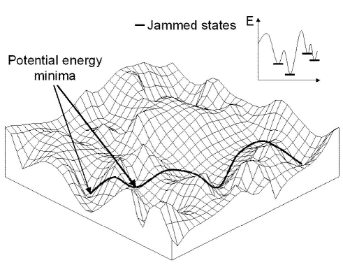
Figure 1: The multidimensional energy landscape dominates the dynamics below the glass transition, as the system explores the inherent structures defined as the potential energy minima. A trajectory through the landscape is shown and the analogy between these inherent structures and the jammed states in granular materials is examined.

The importance of the inherent structure formalism is in enabling the comparison of jamming in particulate systems with glasses [8]. The entropy arising from the inherent configurations of the glass at very low temperatures and the exploration of these configurations due to the vibrational modes of the particles could be viewed as analogous to the configurational changes in particulate packings under slow tapping or shear. However, in granular materials there is an added effect of friction, which dissipates the analogous vibrations at once. Unlike granular materials, a thermal system is never permanently trapped in the bottom of a valley, but escapes in other accessible unstable directions through intrinsic thermal vibrations. At any finite temperature the system will not resemble the granular system in that it continuously evolves toward a maximum density state. Thus, the only true analogous situation between glasses and granular materials is valid at zero temperature. However, there are characteristic features of the glassy relaxation at a finite $T$ which act as useful tools for the description of granular systems by exploiting the analogy between the relaxation of powders and aging in glassy systems [9].

For instance, theories developed during the late eighties and nineties in the field of spin glasses [10, 11] have led to a better understanding of glassy systems through the generalisation of usual equilibrium relations, such as the fluctuation-dissipation relation, to situations far from equilibrium [12]. This approach developed by Cugliandolo, Kurchan and collaborators yielded macroscopic observable properties, such as an “effective temperature” for the slow modes of relaxation, which could then be compared between various glassy systems. Furthermore, the existence of an effective temperature with a thermodynamic meaning in glasses at very low temperature suggests an ‘ergodicity’ for the long-time behaviour of the system [13]. This ergodicity is closely related to the statistical ideas for granular systems [14, 15, 16] which we will introduce in the following sections. In support of this argument, the effective temperature in glasses is found to be an adequate concept for describing granular matter [17], as it will be shown in Section 3.

From a theoretical point of view, these systems are still only understood in terms of predictions of a general nature and many open questions remain. There is still much debate on issues such as the precise mechanisms of surfing the energy landscape, the effects of memory in the system, the slowing down of the system with time, and the discrepancies between the behaviour of different glassy systems, but they are beyond the scope of this work.

2 Jamming in Particulate Systems

In a sense one would imagine there is no simpler physical system than a granular assembly. After all it is just a set of packed rigid objects with no interaction energy. It is the inability to describe the system on the continuum level in any other way except according to its geometry which has led to a lack of a well established granular theory until present. Mostly due to their industrial importance, there has been a vast literature describing phenomenological observations without an encompassing theory. In the words of de Gennes, the state of granular matter can be compared to solid state physics in the 30’s or critical phenomena in phase transitions before the renormalization group. In other words, there is a need for describing the universal features of the observed behaviour within a theoretical framework devised for these and other jammed systems.

In parallel with the extensive research on glasses, described earlier, a decade ago Edwards and collaborators postulated the existence of a statistical ensemble for granular matter, despite the lack of thermal motion and the absence of an equilibrium state [18, 19, 20, 21, 22]. The main postulate was based on jamming the granular particles at a fixed total volume such that all microscopic jammed states are equally probable and become accessible to one another (ergodic hypothesis) by the application of a type of external perturbation such as tapping or shear, just as thermal systems explore their energy landscape through Brownian motion. Hence, let us consider granular jamming in more detail.

Pouring sugar into a cup is the simplest example of a fluid to solid transition which takes place solely because of a density increase. In terms of physics, in particulate materials such as emulsions and granular media, a jammed system results if particles are packed together so that all particles are touching their neighbours, which obviously requires a sufficiently high density. In these athermal systems there is no kinetic energy of consequence; the typical energy required to change the positions of the jammed particles is very large compared to the thermal energy at room temperature ($\sim 10^{14}$ times, see Section 3). As a result, the material remains arrested in a static state and is able to withstand a sufficiently small applied stress.

There is a subtle, but crucial difference, between a configuration in mechanical equilibrium and a jammed configuration, particularly in the context of this research. The mechanism of arriving at a static configuration by an increase in density, which is an intuitively obvious process, is not always sufficient to satisfy the jamming condition in our definition. This applies especially to systems which bear knowledge of the process of their creation. For instance, pouring grains into a container results in a pile at a given angle of repose. This mechanical equilibrium configuration is not jammed because in response to an external perturbation, the constituent particles will irreversibly rearrange, approaching a truly jammed configuration. The statistical mechanics which we are aiming to test implies an ergodic hypothesis, which is not valid in such history-dependent samples .

It turns out that by allowing the system to explore its available configurational space through external mechanical perturbations, the system will rearrange such that all possible configurations (w.r.t. the perturbation) become accessible to one another. Continuing with the analogy in the real world, the gentle tapping on a table of the cup filled with sugar will initially change the unstable angle of repose of the sugar pile and flatten its top surface, and therefore its density, until it settles into a desired configuration which depends on the strength of the tap. We can only perform a statistical analysis on the resulting configurations which have no memory of their creation, i.e. the true jammed configurations. Thus we arrive at a jammed ensemble, suitable for the application of statistical mechanics, described in Section 1. Since the particles can jump across the energy landscape during the tap, but then stop at once due to frictional dissipation, there is an analogy to the inherent structure formalism in glassy systems. This new statistical mechanics is able to provide unifying concepts between previously unrelated media.

1 Applications of the jamming condition

The statistical mechanics which we are aiming to develop implies an ergodic hypothesis, which is not valid in history-dependent samples. In fact, there are many experimental situations in which the statistical mechanics cannot be applied due to the lack of ergodicity. For instance convection cycles have been observed in granular systems under vigorous tapping [24]- an effect which is closely associated with the segregation process of different granular species. These types of closed loops in phase space cannot be described within the thermodynamic framework. Rapid granular flows observed in pouring sand in a pile, or vigorously shaken granular systems at low density are out of the scope of the present approach since the systems are exploring configurations far from the jammed states [25]. Kinetic theories of inelastic gases are more appropriate to treat these situations [26]. The physics of the angle of repose [27] may not be understood under the thermodynamic framework due to the absence of the jamming condition of the pile, despite the fact that it is static. In many practical situations, heterogeneities appear which also preclude the application of a thermodynamic approach. For instance, when granular materials are sheared in a sufficiently large shear stage, shear bands appear where the strain is discontinuous [28]. Such local effects cannot be captured by the present thermodynamic approach.

On the other hand, if the application of statistical physics to jammed phenomena were to prove productive, then one could anticipate a more profound insight into the characterisation and understanding of the system as a whole. For instance, the thermodynamic hypothesis would lead to the prediction of macroscopic quantities such as viscosity and complex shear moduli, which would in turn provide a complete rheological caracterisation of the system. As a matter of theoretical interest, a statistical ensemble for jammed matter could be one of the very few generalisations of the statistical mechanics of Gibbs and Boltzmann to systems out of equilibrium.

2 Achieving the jammed state

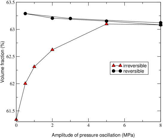
Figure 2: Compaction curve for a packing of glass beads under an oscillating pressure. Increasing the amplitude of oscillation initially increases the density by filling the loose voids, after which a reversible regime is achieved (from [32]).

Experimentally, the conditions for a statistical ensemble of jammed states can be achieved by pre-treating the granular assembly by tapping or via slow shear-driving. Experiments at the University of Chicago involving the tapping of granular columns were the first to show the existence of a reversible regime in which the system configurations are independently sampled [29]. Starting with a loose packing of the grains, the tapping routine initially removes the unstable loose voids and thus eliminates the irreversible grain motion. Once all the grains are touching their neighbours, the density of the resulting configuration becomes dependent on the tapping amplitude and the number of taps; the larger the amplitude, the lower the density. The mechanism of the compaction process leading to a steady-state density is extremely slow, in fact, it is logarithmic in the number of taps. This dependence of the density of grains on the external perturbation of the system once the memory effects of the pile construction details have been removed, is known as the reversible branch of the ‘compaction curve’, see Fig. 2. Despite the presence of friction between grains (implying memory effects) this curve is reversible, establishing a new type of equilibrium states. It is along this curve that the thermodynamics for granular matter can be applied.

There have been several further experiments confirming these results for different system geometries, particle elasticities and compaction techniques. For example, the system can be mechanically tapped or oscillated, vibrated using a loudspeaker, slowly sheared in a couette geometry, or even allowed to relax under large pressures over long periods of time, all to the same effect [30, 31, 32, 33]. Here we show a new compaction regime under an oscillating pressure where the same density dependence of a packing of glass and acrylic beads is noted for varying amplitudes of the pressure oscillation. These experiments have been performed at Schlumberger-Doll Research [32]. The resulting curve of the achieved volume fraction as a function of the amplitude of the pressure oscillation is shown in Fig. 2.

Moreover, experiments in the Cavendish laboratory [33] have shown how the conductivity of powdered graphite can also be a measure of the particle density as it is being vibrated, in which the direct link to the volume function is less obvious, but the qualitative results indicate the same trends. The methodology for achieving jammed configurations has also been established numerically for the purpose of rheological and thermodynamical studies and it will be described in Section 3.

At this point, it is important to note that we have only considered infinitely rigid, rough grains in which an increase in the pressure of the system, for instance by placing a piston on top of the grains, causes no change in the shape of the grains and therefore no change in the packing density. On the other hand, real grains have a finite elastic modulus, thus the application of a sufficiently large external pressure will always result in grain deformation and therefore a density increase unrelated to the tapping. In soft particles, such as emulsions, the effect of pressure is more significant. The tapping experiment described above measured the resulting densities at atmospheric pressure, which is considered to be the zero reference pressure. The same experiment can be repeated at finite pressures giving rise to equivalent compaction curves, depicted in Fig. 3. Whereas hard grains, such as glass beads, require extremely large pressures ($\sim 1$MPa) to deform and the amount of deformation is limited by their yield stress, softer particles, such as rubber, are able to reach higher densities with relative ease. Droplets and bubbles, being the softest particles one can have, are capable of reaching the density of 1, corresponding to a biliquid foam and a foam, respectively, by an application of much smaller pressures ($\sim 1$kPa). They have the advantage of the whole pressure range being accessible to them. Another distinction between granular materials and emulsions is the presence of friction in the former and the smoothness of the latter. Since friction plays an important role in inducing memory into the system, its absence leads to a much easier achievement of the jammed state, described above. For instance, in the case of emulsions, allowing the particles to cream under gravity will suffice to arrive at the reversible part of the compaction curve, bypassing the irreversible branch as it will be shown in Section 2.

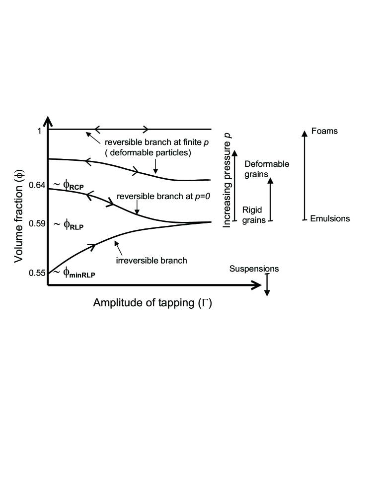
Figure 3: Compaction curves of volume fraction $\phi$ versus amplitude of oscillation $\Gamma$ for different external confining pressures, $p$. Increasing the amplitude of oscillation initially increases the volume fraction by filling the loose voids (irreversible branch), after which a reversible regime is achieved. For infinitely rigid grains (the “zero pressure” curve) the minimum volume fraction along the irrevesible branch is the random loose packing. The reversible branch goes from the random loose packing fraction to the random close packing fraction. Below the minimum RLP only suspensions can exist.

3 Unifying Concepts in Granular Matter and Glasses

In the preceding paragraphs, it has been shown under which conditions both thermal and athermal systems explore the configurational energy landscape, which possibly results in commonalities in their behaviour. At present, new unifying theoretical descriptions for jammed matter are being sought, as well as new experimental evidence to unify the predicted state for all varieties of jammed systems.

The prediction of how different systems jam with respect to the applied stress, density and temperature has led to a speculative diagram proposed by Liu and Nagel in their article “Jamming is not just cool anymore” in Nature [34, 35, 36]. It links the behaviour of glasses (thermal systems) and bubbles, grains, droplets (athermal systems) by the dynamics of their approach to jamming.

Since the observable properties such as applied strain, temperature and density can be obtained by consideration of only the jammed configurations in a given system, the thermodynamics of jamming, discussed in the next section, is intimately related to the ideas put forward in the jamming phase diagram.

Chapter 1 New Statistical Mechanics for Granular Matter

This Section aims to justify the use of statistical mechanics tools in situations where the system is far from thermal equilibrium, but jammed. In what follows, we present the classical statistical mechanics theorems to an extent which facilitates an understanding of the important concepts for the development of an analogous granular theory, as well as the assumptions necessary for the belief in such a parallel approach. Thereafter, we present a theoretical framework to fully describe the exact specificities of the granular packing, and the shaking scenario which leads to the derivation of the Boltzmann equation for a jammed granular system.

This kind of an analysis paves the path to macroscopic quantities, such as the compactivity, characterising the configurations from the microstructural information of the packing. It is according to this theory that the jammed configurations obtained from experiments and simulations are later characterised.

1 Classical Statistical Mechanics

In the conventional statistical mechanics of thermal systems, the different possible configurations, or microstates, of the system are given by points in the phase space of all positions and momenta {$p,q$} of the constituent particles. The equilibrium probability density $\rho_{\mbox{\scriptsize eqm}}$ must be a stationary state of Liouville’s equation which implies that $\rho_{\mbox{\scriptsize eqm}}$ must be expressed only in terms of the total energy of the system, $E$ [37]. The simplest form for a system with Hamiltonian ${\cal H}(p,q)$ is the microcanonical distribution:

$$\rho_{\mbox{\scriptsize eqm}}(E)=\frac{1}{\Sigma_{\mbox{\scriptsize eqm}}(E)},$$ (1)

for the microstates within the ensemble, ${\cal H}(p,q)=E$, and zero otherwise. Here,

$$\Sigma_{\mbox{\scriptsize eqm}}(E)=\int\delta\Big{(}E-{\cal H}(p,q)\Big{)}~{}~{}dp~{}dq,$$ (2)

is the area of energy surface ${\cal H}(p,q)=E$.

Equation (1) states that all microstates are equally probable. Assuming that this is the true distribution of the system implies accepting the ergodic hypothesis, i.e. the trajectory of the closed system will pass arbitrarily close to any point in phase space.

It was the remarkable step of Boltzmann to associate this statistical concept of the number of microstates with the thermodynamic notion of entropy through his famous formula

$$S_{\mbox{\scriptsize eqm}}(E)=k_{B}\ln\Sigma_{\mbox{\scriptsize eqm}}(E).$$ (3)

Thus, in classical statistical mechanics, the total energy of the system is sufficient to describe the probability density of states. Whereas the study of thermal systems has had the advantage of available statistical mechanics tools for the exploration of the phase space, an entirely new statistical method, unrelated to the temperature, had to be constructed for grains.

2 Statistical Mechanics for Jammed Matter

We now consider a jammed granular system composed of rigid grains (deformable particles will be considered in Section 3). Such a system is analogously described by a network of contacts between the constituent particles in a fixed volume, $V$, since there is no relevant energy $E$ in the system. In the case of granular materials, the analogue of phase space, the space of microstates of the system, is the space of possible jammed configurations as a function of the degrees of freedom of the system $\{\zeta\}$.

It is argued that it is the volume of this system, rather than the energy, which is the key macroscopic quantity governing the behaviour of granular matter [18, 19, 20]. If we have $N$ grains of specified shape which are assumed to be infinitely rigid, the system’s statistics would be defined by a function ${\cal W}(\zeta)$, a function which gives the volume of the system in terms of the specification of the grains.

In this analogy one replaces the Hamiltonian ${\cal H}(p,q)$ of the system by the volume function, ${\cal W}(\zeta)$. The average of ${\cal W}(\zeta)$ over all the jammed configurations determines the volume $V$ of the system in the same way as the average of the Hamiltonian determines the average energy $E$ of the system.

1 Definition of the volume function, $\cal W$

One of the key questions in this analogy is to establish the ‘correct’ $\cal W$ function, the statistics of which is capable of fully describing the system as a whole. The idea is to partition the volume of the system into different subsystems $\alpha$ with volume ${\cal W}^{\alpha}$, such that the total volume of a particular configuration is

$${\cal W}(\zeta)=\sum_{\alpha}{\cal W}^{\alpha}.$$ (4)

It could be that considering the volume of the first coordination shell of particles around each grain is sufficient; thus, we may identify the partition $\alpha$ with each grain. However, particles further away may also play a role in the collective system response due to enduring contacts, in which case $\cal W$ should encompass further coordination shells. In reality, of course, the collective nature of the system induces contributions from grains which are indeed further away from the grain in question, but the consideration of only its nearest neighbours is a good starting point for solving the system, and is the way in which we proceed to describe the $\cal W$ function. The significance of the appropriate definition of $\cal W$ is best understood by the consideration of a response to an external perturbation to the system in terms of analogies with the Boltzmann equation which we will describe in Section 4.

Perhaps the most straightforward definition of the function ${\cal W}^{\alpha}$ is given in terms of the Voronoi diagram which partitions the space into a set of regions, associating all grain centroids in each region to the closest grain centroid, depicted by line OP in the diagram in Fig. 1a. The loop formed by the perpendicular bisectors (ab) of each of the lines joining the central grain to its neighbours is the Voronoi cell, depicted in red. Even though this construction successfully tiles the system, its drawback is that there is no analytical formula for the enclosed volume of each cell. Recently Ball and Blumenfeld [38, 39] have shown by an exact triangulation method that the volume defining each grain can be given in terms of the contact points C using vectors constructed from them (see Fig. 1b). The method consists in defining shortest loops of grains in contact with one another (p,q loops), thus defining the void space around the central grain. The difficulty arises in three dimensions since this construction requires the identification of void centres, v. This is not an obvious task, but is currently under consideration. The resulting volume (red) is the antisymmetric part of the fabric tensor, the significance of which is its appearance in the calculation of stress transmission through granular packings [38].

A cruder version for the volume per grain, yet with a strong physical meaning, has been given by Edwards. For a pair of grains in contact (assumed to be point contacts for rough, rigid grains) the grains are labelled $\alpha,\beta$, and the vector from the centre of $\alpha$ to that of $\beta$ is denoted as ${\rm\bf R}^{\,\alpha\beta}$ and specifies the complete geometrical information of the packing. The first step is to construct a configurational tensor ${\rm\bf\cal C}^{\alpha}$ associated with each grain $\alpha$ based on the structural information,

$${\cal C}_{ij}^{\alpha}=\sum_{\beta}R_{i}^{\alpha\beta}R_{j}^{\alpha\beta}.$$ (5)

Then an approximation for the area in 2D or volume in 3D encompassing the first coordination shell of the grain in question is given as

$${\cal W}^{\alpha}=2\sqrt{\mbox{Det}~{}{\cal C}_{ij}^{\alpha}}.$$ (6)

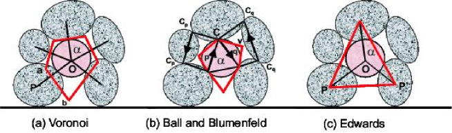
Figure 1: Different volume functions as discussed in the text: (a) Voronoi, (b) Ball and Blumenfeld and (c) Edwards construction.

This volume function is depicted in the Fig. 1c, with grain coordination number 3 in two dimensions, where Eq. (6) should give the area of the triangle (red) constructed by the centres of grains P which are in contact with the grain $\alpha$. The above equation is exact if the area is considered as the determinant of the vector cross product matrix of the two sides of the triangle, but its validity for higher coordination numbers and in 3D has not been tested. Surprisingly, this approximation works well according to our experimental studies in Section 2. This is due to the partitioning of the obtained volumetric objects into triangles/pyramids, intrinsic to the method, and subsequently summing over them to obtain the resulting volume.

This definition is clearly only an approximation of the space available to each grain since there is an overlap of ${\cal W}^{\alpha}$ for grains belonging to the same coordination shell. Thus, it overestimates the total volume of the system: $\sum{\cal W}^{\alpha}>V$. However, it is the simplest approximation for the system based on a single coordination shell of a grain.

2 Entropy and compactivity

Now that we have explicitly defined $\cal W$ it is possible to define the entropy of the granular packing. The number of microstates for a given volume $V$ is measured by the area of the surface ${\cal W}(\zeta)=V$ in the phase space of jammed configurations and it is given by:

$$\Sigma_{\mbox{\scriptsize jammed}}(V)=\int\delta\Big{(}V-{\cal W}(\zeta)\Big{)}~{}~{}\Theta(\zeta)~{}~{}d\zeta,$$ (7)

where now $d\zeta$ refers to an integral over all possible jammed configurations and $\delta(V-{\cal W}(\zeta))$ formally imposes the constraint to the states in the sub-space ${\cal W}(\zeta)=V$. $\Theta(\zeta)$ is a constraint that restricts the summation to only reversible jammed configurations as opposed to the merely static equilibrium configurations as previously discussed. This function will be discussed in detail in Section 2. The radical step is the assumption of equally probable microstates which leads to an analogous thermodynamic entropy associated with this statistical quantity:

$$S(V)=\lambda\ln\Sigma_{\mbox{\scriptsize jammed}}(V)=\lambda\ln\int\delta\Big{(}V-{\cal W}(\zeta)\Big{)}~{}~{}\Theta(\zeta)~{}~{}d\zeta,$$ (8)

which governs the macroscopic behaviour of the system [20, 19]. Here $\lambda$ plays the role of the Boltzmann constant. The corresponding analogue of temperature, named the “compactivity”, is defined as

$$X_{V}^{-1}=\frac{{\partial S}}{{\partial V}}.$$ (9)

where the subscript $V$ refers to the fact that it is the derivative of the entropy with respect to the volume.

This is a bold statement, which perhaps requires further explanation in terms of the actual role of compactivity in describing granular systems. We can think of the compactivity as a measure of how much more compact the system could be, i.e. a large compactivity implies a loose configuration (e.g. random loose packing, RLP) while a reduced compactivity implies a more compact structure (e.g. random close packing, RCP, the densest possible random packing of monodisperse hard spheres). In terms of the reversible branch of the compaction curve, large amplitudes generate packings of high compactivities, while in the limit of the amplitude going to zero a low compactivity is achieved. In terms of the entropy, many more configurations are available at high compactivity, thus the dependence of the entropy on the volume fraction can be qualitatively described as in Fig. 2. In the figure, for monodisperse packings the RCP is identified at $\phi\approx 0.64$ [40], the RLP fraction is identified at $\phi\approx 0.59$ [41], while the crystalline packing, FCC, is at $\phi=0.74$ but cannot be reached by tapping.

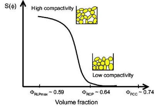
Figure 2: Interpretation of the compactivity and entropy in terms of different packings. See also Fig. 2.

At any given tapping amplitude, there exists an equilibrium volume fraction toward which the system slowly evolves. For instance, a system may find itself at a lower entropy than the equilibrium curve by the application of an internal constraint at a given volume fraction. This situation can be achieved by creating small crystalline regions within a packing configuration of a lower density, and looser regions compensating for the volume reduction such that the total volume of the system remains constant. This configuration, given that it is not jammed, will tend toward the equilibrium packing via the application of a small perturbation by increasing its entropy. Such an example will be made more explicit in the derivation of the Boltzmann equation for granular materials. At volume fractions beyond the RCP (and at atmospheric pressure) the system is not able to explore the configurations as they can only be achieved by the partial crystallisation of the sample, where there are very few configurations available.

It becomes clear from Eq. (9) that the compactivity is only applicable in equilibrated jammed states. As an analogue of temperature, it should also obey the zero-th law of thermodynamics. Hence, two different powders in physical contact with one another should equilibrate at the same compactivity, given a mechanism of momentum transfer between the two systems. Indeed, we may think of an appropriate laboratory experiment which would test this hypothesis under certain conditions necessary for creating the analogous situation to heat flow.

Two powders, A and B, of different grain types are poured into a vertical couette cell as shown in Fig. 3. The grains must experience an equivalent tapping or shearing regime, which is achieved by the rotation of the inner cylinder of the couette cell. The species are separated by a flexible diaphragm, such that momentum transfer between the two systems is ensured. The two powders must be well separated such that there is no mixing involved, but in contact nevertheless. The grains are kept at a constant pressure by a piston which is allowed to move freely to accommodate for the changes in volume experienced by the two types of grains. Gravity may play a role in the experiment, which is avoided by density matching the particles with a suspending fluid.

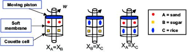
Figure 3: ABC experiment to test the zero-th law of granular thermodynamics.

The experiment consists in placing powders A and B together in the above cell and slowly shearing them at a given velocity. The powders should come to equilibrium volumes $V_{A}$ and $V_{B}$, with equivalent respective compactivities, $X_{A}=X_{B}=X$. While it is easy to measure the volumes of the two systems, the measurement of their compactivities employs more sophisticated methods, discussed in Section 3. In the absence of a compactivity scale, we use powder B as a ‘thermometer’ by placing it in contact with a third powder C. The volume B is kept at $V_{B}$ and the volume of C is allowed to fluctuate until it reaches the equilibrium state. Finally, powders A and C are put together to test if they will reach the same volumes as they did in previous runs in contact with B, thus proving the zero-th law. A form of the zero-th law of thermodynamics will be shown to be valid numerically in Section 3.

3 Remarks

To summarise, the granular thermodynamics is based on two postulates:

1) While in the Gibbs construction one assumes that the physical quantities are obtained as an average over all possible configurations at a given energy, the granular ensemble consists of only the jammed configurations at the appropriate volume.

2) As in the microcanonical equilibrium ensemble, the strong ergodic hypothesis is that all jammed configurations of a given volume can be taken to have equal statistical probabilities.

The ergodic hypothesis for granular matter was treated with skepticism, mainly because a real powder bears knowledge of its formation and the experiments are therefore history dependent. Thus, any problem in soil mechanics or even a controlled pouring of a sand pile does not satisfy the condition of all jammed states being accessible to one another as ergodicity has not been achieved, and the thermodynamic picture is therefore not valid. This point has been discussed in Section 2. The Chicago experiments of tapping columns [30] showed the existence of reversible situations. For instance, let the volume of the column be $V(n,\Gamma)$ where $n$ is the number of taps and $\Gamma$ is the strength of the tap. If one first obtain a volume $V(n_{1},\Gamma_{1})$, and then repeat the experiment at a different tap intensity and obtain $V(n_{2},\Gamma_{2})$, when we return to tapping at $(n_{1},\Gamma_{1})$ one obtains a volume $V^{\prime}$ which is $V^{\prime}(n_{1},\Gamma_{1})=V(n_{1},\Gamma_{1})$. Moreover, in simulations of slowly sheared granular systems the ergodic hypothesis was shown to work [17] as we will discuss in Section 3.

It is often noted in the literature that although the simple concept of summing over all jammed states which occupy a volume $V$ works, there is no first principle derivation of the probability distribution of the Edwards ensemble as it is provided by Liouville’s theorem for equilibrium statistical mechanics of liquids and gases. In granular thermodynamics there is no justification for the use of the $\cal W$ function to describe the system as Liouville’s theorem justifies the use of the energy in the microcanonical ensemble. In Section 4 we will provide an intuitive proof for the use of $\cal W$ in granular thermodynamics by the analogous proof of the Boltzmann equation.

The comment was also made that there is no proof that the entropy Eq. (8) is a rigorous basis for granular statistical mechanics. In the next section we will develop a Boltzmann equation for jammed systems and show that this analysis can be used to produce a second law of thermodynamics, $\delta S\geq 0$ for granular matter, and the equality only comes with Eq. (8) being achieved.

Although everyone believes that the second law of thermodynamics is universally true in thermal systems, the only accessible proof comes in the Boltzmann equation, as the ergodic theory is a difficult branch of mathematics which will not be covered in the present discussion. By investigating the assumptions and key points which led to the derivation of the Boltzmann equation in thermal systems, it is possible to draw analogies for an equivalent derivation in jammed systems.

It should be noted that there is an extensive literature on granular gases [25, 26], which are observed when particles are fluidised by vigorous shaking, thus inducing continuous particle collisions. There is a powerful literature on this topic, but it is not applicable to the problem of jamming.

3 The Classical Boltzmann Equation

Entropy in thermal systems satisfies the second law,

$$\frac{\partial S}{\partial t}\geq 0,$$ (10)

which states that there is a maximum entropy state which, according to the evolution in Eq. (10), any system evolves toward, and reaches at equilibrium. A ‘semi’-rigorous proof of the Second Law was provided by Boltzmann (the well-known ‘H-theorem’), by making use of the ‘classical Boltzmann equation’, as it is now known.

In order to derive this equation, Boltzmann made a number of plausible assumptions concerning the interactions of particles, without proving them rigorously. The most important of these assumptions were:

• The collision processes are dominated by two-body collisions (Fig. 4a). This is a plausible assumption for a dilute gas, since the system is of very low density, and the probability of there being three or more particles colliding is infinitesimal.

• Collision processes are uncorrelated, i.e. all memory of the collision is lost on completion and is not remembered in subsequent collisions: the famous Stosszahlansatz. This is also valid only for dilute gases, but the proof is more subtle.

Thus, Boltzmann proves Eq. (10) for a dilute gas only, but this is a readily available situation. The remaining assumptions have to do with the kinematics of particle collisions, i.e. conservation of kinetic energy, conservation of momentum, and certain symmetry of the particle scattering cross-sections.

Let $f(v,r)$ denote the probability of a particle having a velocity $v$ at position $r$. This probability changes in time by virtue of the collisions. The two particle collision is visualised in Fig. 4a where $v$ and $v_{1}$ are the velocities of the particles before the collision and $v^{\prime}$ and $v^{\prime}_{1}$ after the collision.

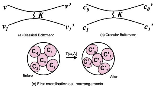
Figure 4: (a) Collision of two particles in a dilute gas. (b) “Collision of two configurations” given in terms of two contact points in a jammed material. (c) Rearrangements inside a pocket of mobile grains under the first coordination shell approximation for grain $\alpha=0$.

On time scales larger than the collision time, momentum and kinetic energy conservation apply:

$$mv+mv_{1}=mv^{\prime}+mv_{1}^{\prime},\\ \\ \\ \\ \\ \\ \\ \\ \\ \ \frac{1}{2}mv^{2}+\frac{1}{2}mv_{1}^{2}=\frac{1}{2}mv^{\prime 2}+\frac{1}{2}m{v^{\prime}}_{1}^{2}.$$ (11)

Then, the distribution $f(v,r)$ evolves with time according to

$$\frac{\partial f}{\partial t}+v\frac{\partial f}{\partial r}+\int{\cal K}(v,v^{\prime};v_{1},v_{1}^{\prime})~{}~{}\Big{(}f(v)f(v_{1})-f(v^{\prime})f(v_{1}^{\prime})\Big{)}~{}~{}d^{3}v_{1}d^{3}v^{\prime}d^{3}v_{1}^{\prime}=0.$$ (12)

The kernel $\cal K$ is positive definite and contains $\delta$-functions to satisfy the conditions (11), the flux of particles into the collision and the differential scattering cross-section. We consider the case of homogeneous systems, i.e. $f=f(v)$, and define

$$S=-k_{B}\int f\ln f.$$ (13)

Defining $x=ff_{1}/f^{\prime}f^{\prime}_{1}$ we obtain

$$\frac{\partial S}{\partial t}=\int{\cal K}~{}\ln x~{}(1-x)d^{3}v_{1}~{}d^{3}v^{\prime}~{}d^{3}v_{1}^{\prime},\\ (1-x)\ln x\geq 0,\\ {\cal K}\geq 0.$$ (14)

Hence $\partial S/\partial t\geq 0$ (see standard text books on statistical mechanics).

It is also straightforward to establish the equilibrium distribution where $\partial S/\partial t=0$ since it occurs when the kernel term vanishes, i.e. when the condition of detailed balance is achieved, $x=1$:

$$f(v)f(v_{1})=f(v^{\prime})f(v_{1}^{\prime}).$$ (15)

The solution of Eq. (15) subjected to the condition of kinetic energy conservation is given by the Boltzmann distribution

$${\displaystyle f(v)=\left(\frac{k_{B}T}{m\pi}\right)^{3/2}~{}e^{-\frac{1}{2}\beta mv^{2}}},$$ (16)

where $\beta=1/k_{B}T$. Equation (16) is a reduced distribution and valid only for a dilute gas. The Gibbs distribution represents the full distribution and is obtained by replacing the kinetic energy in (16) by the total energy of the state to obtain:

$$P(E)\propto e^{-\beta E}.$$ (17)

The question is whether a similar form can be obtained in a granular system in which we expect

$$P({\cal W})\propto e^{-{\cal W}/\lambda X},$$ (18)

where $X$ is the compactivity in analogy with $T=\partial{E}/\partial{S}$. Such an analysis is shown in the next section in an approximate manner.

4 ‘Boltzmann Approach’ to Granular Matter

The analogous approach to granular materials consists in the following: the creation of an ergodic grain pile suitable for a statistical mechanics approach via a method for the exploration of the available configurations analogous to Brownian motion, the definition of the discrete elements tiling the granular system via the volume function $\cal W$ (the sum of which provides the analogous ‘Hamiltonian’ to the energy in thermal systems), and an equivalent argument for the energy conservation expressed in terms of the system volume necessary for the construction of the Boltzmann equation.

We have already established the necessity of preparing a granular system adequate for real statistical mechanics so as to emulate ergodic conditions. The grain motion must be well-controlled, as the configurations available to the system will be dependent upon the amount of energy/power put into the system. This pretreatment is analogous to the averaging which takes place inherently in a thermal system and is governed by temperature.

As explained, the granular system explores the configurational landscape by the external tapping introduced by the experimentalist. The tapping is characterised by a frequency and an amplitude ($\omega,\Gamma$) which cause changes in the contact network, according to the strength of the tap. The magnitude of the forces between particles in mechanical equilibrium and their confinement determine whether each particle will move or not. The criterion of whether a particular grain in the pile will move in response to the perturbation will be the Mohr-Coulomb condition of a threshold force, above which sliding of contacts can occur and below which there can be no changes. The determination of this threshold involves many parameters, but it suffices to say that a rearrangement will occur between those grains in the pile whose configuration and neighbours produce a force which is overcome by the external disturbance.

The concept of a threshold force necessary to move the particles implies that there are regions in the sample in which the contact network changes and those which are unperturbed, shown in Fig. 5. Of course, since this is a description of a collective motion behaviour, the region which can move may expand or contract, but the picture at any moment in time will contain pockets of motion encircled by a static matrix. Each of these pockets has a perimeter, defined by the immobile grains. It is then possible to consider the configuration before and after the disturbance inside this well-defined geometry.

The present derivation assumes the existence of these regions. It is equivalent to the assumption of a dilute gas in the classical Boltzmann equation, although the latter is readily achieved experimentally.

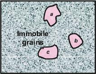
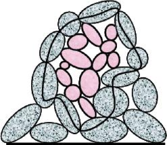
Figure 5: (a) Regions of mobile grains $a,b,c$ in a matrix of immobile grains below the Coulomb threshold. (b) Detail of pocket of mobile grains $a$ surrounded by immobile grains which are shaded.

The energy input must be on the level of noise, such that the grains largely remain in contact with one another, but are able to explore the energy landscape over a long period of time. In the case of external vibrations, the appropriate frequency and amplitude can be determined experimentally for different grain types, by investigating the motion of the individual grains or by monitoring the changes in the overall volume fraction over time. It is important that the amplitude does not exceed the gravitational force, or else the grains are free to fly up in the air, re-introducing the problem of initial creation just as they would if they were simply poured into another container.

Within a region $a$ we have a volume $\sum_{\alpha\in a}{\cal W}^{\alpha}$ and after the disturbance a volume which is now $\sum_{\alpha\in a}{\cal W}^{\prime\alpha}$ as seen in Fig. 4b and 4c. In Section 1 we have discussed how to define the volume function ${\cal W}^{\alpha}$ as a function of the contact network. Here the simplest “one grain” approximation is used as the “Hamiltonian” of the volume as defined by Eq. (6). In reality it is much more complicated, and although there is only one label $\alpha$ on the contribution of grain $\alpha$ to the volume, the characteristics of its neighbours may also appear.

Instead of energy being conserved, it is the total volume which is conserved while the internal rearrangements take place within the pockets described above. Hence

$$\sum_{\alpha\in a}{{\cal W}^{\alpha}}=\sum_{\alpha\in a}{{\cal W}^{\prime\alpha}}.$$ (19)

We now construct a Boltzmann equation. Suppose $z$ particles are in contact with grain $\alpha=0$, as seen in Fig. 4c. For rough particles $z=4$ while for smooth $z=6$ at the isostatic limit (see Section 3). The probability distribution will be of the packing configurations which are represented by the tensor ${\cal C}^{\alpha}$, Eq. (5), for each grain, where $\alpha$ ranges from 0 to 4 in this case. So the analogy of $f(v)$ for the Boltzmann gas equation becomes $f({\cal C}^{0})$ for the granular system and represents the probability that the external disturbance causes a particular motion of the grain. We therefore wish to derive an equation

$$\frac{\partial f({\cal C}^{0})}{\partial t}+\int{\cal K}({\cal C}^{\alpha},{\cal C}^{\prime\alpha})~{}~{}\Big{(}f_{0}f_{1}f_{2}f_{3}f_{4}-f^{\prime}_{0}f^{\prime}_{1}f^{\prime}_{2}f^{\prime}_{3}f^{\prime}_{4}\Big{)}~{}~{}d{\cal C}^{\prime 0}\prod_{\alpha\neq 0}d{\cal C}^{\alpha}d{\cal C}^{\prime\alpha}=0.$$ (20)

The term $\cal K$ contains the condition that the volume is conserved (19), i.e. it must contain $\delta(\sum{\cal W}^{\alpha}-\sum{\cal W}^{\prime\alpha})$. The cross-section is now the compatibility of the changes in the contacts, i.e. ${\cal C}^{\alpha}$ must be replaced in a rearrangement by ${\cal C}^{\prime\alpha}$, Fig. 4b (unless these grains part and make new contacts in which case a more complex analysis is called for). We therefore argue that the simplest $\cal K$ will depend on the external disturbance $\Gamma,\omega$ and on ${\cal C}^{\alpha}$ and ${\cal C}^{\prime\alpha}$, i.e.

$$\frac{\partial f({\cal C}^{0})}{\partial t}+\int\delta\Big{(}\sum_{\alpha}{\cal W}^{\alpha}-\sum_{\alpha}{\cal W}^{\prime\alpha}\Big{)}~{}{\cal J}({\cal C}^{\alpha},{\cal C}^{\prime\alpha})~{}~{}\Big{(}\prod_{\alpha=0}^{z}f_{\alpha}-\prod_{\alpha=0}^{z}f^{\prime}_{\alpha}\Big{)}~{}d{\cal C}^{\prime 0}\prod_{\alpha\neq 0}d{\cal C}^{\alpha}d{\cal C}^{\prime\alpha}=0.$$ (21)

where $\cal J$ is the cross-section and it is positive definite.

The Boltzmann argument now follows. As before

$$S=-\lambda\int f\ln f,\\ x=\frac{f_{0}f_{1}f_{2}f_{3}f_{4}}{f_{0}^{\prime}f_{1}^{\prime}f_{2}^{\prime}f_{3}^{\prime}f_{4}^{\prime}},$$ (22)

and

$$\frac{\partial S}{\partial t}\geq 0,$$ (23)

the equality sign being achieved when $x=1$ and

$$f_{\alpha}=\frac{e^{-{\cal W}^{\alpha}/\lambda X}}{Z},$$ (24)

with the partition function

$$Z=\sum_{\alpha}e^{-{\cal W}^{\alpha}/\lambda X}~{}~{}~{}{\Theta_{\alpha}},$$ (25)

and the analogue to the free energy being $Y=-X\ln Z$, and $X=\partial V/\partial S$.

The detailed description of the kernel $\cal K$ has not been derived as yet due to its complexity. Just as Boltzmann’s proof does not depend on the differential scattering cross section, only on the conservation of energy, in the granular problem we consider the steady state excitation externally which conserves volume, leading to the granular distribution function, Eq. (24).

It is interesting to note that there is a vast and successful literature of equilibrium statistical mechanics based on $\exp(-{\cal H}/k_{B}T)$, but a meagre literature on dynamics based on attempts to generalise the Boltzmann equation or, indeed, even to solve the Boltzmann equation in situations remote from equilibrium where it is still completely valid. It means that any advancement in understanding how it applies to analogous situations is a step forward.

Chapter 2 Jamming with the Confocal

1 From Micromechanics to Thermodynamics

The first step in realising the idea of a general jamming theory is to understand in detail the characteristics of jammed configurations in particulate systems. Thus, the main aim of this section is to design an experiment to provide a microscopic foundation for the statistical mechanics of jammed systems. The understanding of the micromechanics on the scale of the particle, together with the respective statistical measures, pave the path towards an experimental proof of the existence of such an underlying thermodynamics.

The problem with the characterisation of the jammed state in terms of its microstructure is that the condition of jamming implies an optically impenetrable particulate packing. The fact that we cannot take a look inside the bulk to infer the structural features has confined all but one three-dimensional study of packings to numerical simulations and the walls of an assembly. In the old days Mason, a graduate student of Bernal, took on the laborious task of shaking glass balls in a sack and ‘freezing’ the resulting configuration by pouring wax over the whole system. He would then carefully take the packing apart, ball by ball, noting the positions of contacts (ring marks left by the wax) for each particle [40]. The statistical analysis of his hard-earned data led to the reconstruction of the contact network in real space, a measurement of the radial distribution function, $g(r)$, and also the number of contacts of each particle satisfying mechanical equilibrium which gives $z\approx 6.4$ for close contacts. This has been the only reference point for simulators and theoreticians to compare their results with those from the real world and it therefore deserves a particular mention.

In search of an alternative method of experimentation, more in line with the automated nature of our times, we developed a model system suitable for optical observation. Moreover, our aim was to investigate the jammed state in a different jammed medium, to probe the universality of the configurational features. Finally, one needs to solve the system geometry as well as the stresses propagating through it in order to come up with a general theory. To probe the stress propagation through the medium, rather than its configuration alone, the particles must have well-defined elastic properties. The system which could satisfy all our requirements was found in a packing of emulsion droplets [42, 43].

2 Model system

Emulsions are a class of material which is both industrially important and exhibits very interesting physics [44]. They belong to a wider material class of colloids in that they consist of two immiscible phases one of which is dispersed into the other, the continuous phase. Both of the phases are liquids and their interface is stabilised by the presence of surface-active species.

Emulsions are amenable to our study of jamming due to the following properties:

Transparency.

An alternative way of ‘seeing through’ the packing is to refractive index match the phases in the system - i.e. the particles and the continuous medium filling the voids. Since an emulsion is made up of two immiscible liquids, it is possible to raise the refractive index of the aqueous phase to match that of the dispersion of oil droplets. However, transparency is not the only requirement, since the particles are then dyed to allow for their optical detection.

Alternative Medium.

The emulsion is made up of smooth, stable droplets in the $1-10\mu$m size range, as compared to rigid, rough particles in the above described granular system. Both systems are athermal, but the length scale and the properties of the constituent particles of the system are very different.

Elasticity.

Emulsion droplets are deformable, stabilised by an elastic surfactant film, which allows for the measurement of the interdroplet forces from the amount of film deformation upon contact. Moreover, the elasticity facilitates the measurement of the dependence of the contact force network on the external pressure applied to the system.

Our model system consists of a dense packing of emulsion oil droplets, with a sufficiently elastic surfactant stabilising layer to mimic solid particle behaviour, suspended in a continuous phase fluid. The refractive index matching of the two phases, necessary for 3D imaging, is not a trivial task since it involves unfavourable additions to the water phase, disturbing surfactant activity. The successful emulsion system, stable to coalescence and Ostwald ripening, consisted of Silicone oil droplets ($\eta=10$cS) in a refractive index matching solution of water ($w_{t}=51\%$) and glycerol ($w_{t}=49\%$), stabilised by 20$mM$ sodium dodecylsulphate (SDS) upon emulsification and later diluted to below the critical micellar concentration (CMC$=13mM$) to ensure a repulsive interdroplet potential. The droplet phase is fluorescently dyed using Nile Red, prior to emulsification. The control of the particle size distribution, prior to imaging, is achieved by applying very high shear rates to the sample, inducing droplet break-up down to a radius mean size of $3.4\mu m$. This system is a modification of the emulsion reported by Mason et al. [45] to produce a transparent sample suitable for confocal microscopy.

1 Characterisation of a jammed state

Having prepared a stable, transparent emulsion we use confocal microscopy for the imaging of the droplet packings at varying external pressures, i.e. volume fractions. The key feature of this optical microscopy technique is that only light from the focal plane is detected. Thus 3D images of translucent samples can be acquired by moving the sample through the focal plane of the objective and acquiring a sequence of 2D images.

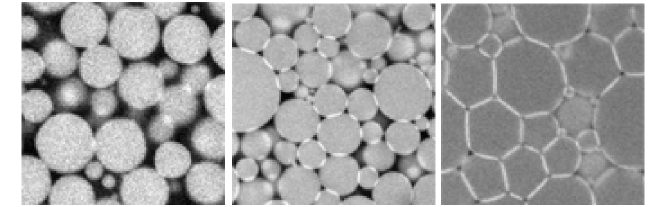
Figure 1: 2D slices of emulsions under varying compression rates: (a) 1g, (b) 6000g, and (c) 8000g.

Since the emulsion components have different densities, the droplets cream under gravity to form a random close packed structure. In addition, the absence of friction ensures that the system has no memory effects and reaches a true jammed state before measurement. If the particles are subjected to ultracentrifugation, configurations of a higher density are achieved as the osmotic pressure is increased. The random close packing fraction reached under gravity depends on the polydispersity of the emulsion, or in other words, the efficiency of the packing. The sequence of images in Fig. 1 shows 2D slices from the middle of the sample volume after: (a) creaming under gravity, (b) centrifugation at 6000g for 20 minutes and (c) centrifugation at 8000g for 20 minutes. The samples were left to equilibrate for several hours prior to measurements being taken.

The volume fraction for our polydisperse system shown in Fig. 1b is $\phi=0.86$, determined by image analysis. This high volume fraction obtained at a relatively small osmotic pressure of 125 Pa is achieved due to the polydispersity of the sample.

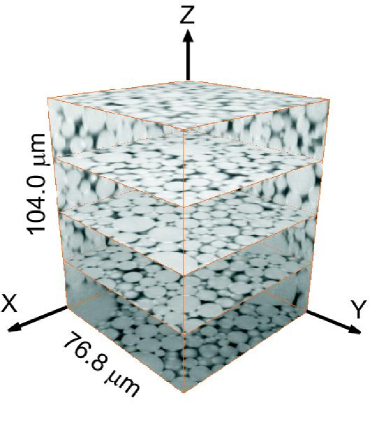
Figure 2: Confocal image of the densely packed emulsion system.

The 3D reconstruction of the 2D slices is shown in Fig. 2. We have developed a sophisticated image analysis algorithm which uses Fourier Filtering to determine the particle centres and radii with subvoxel accuracy of all the droplets in the sample [42]. This data was previously unavailable from true 3D experiments. Since the droplets are deformable and they exert forces on one another upon contact, the area of droplet deformation gives an approximation of the force. The deformed areas appear brighter than the rest of the image due to an enhanced fluorescence at the contact [42], allowing for an independent measurement of the forces between droplets as can clearly be seen in Fig. 3.

A system of random close packed particles is fully described by the geometry of the system configuration and the distribution of forces and stresses in the particulate medium. This means that if $P$ is the probability distribution of configurations and of interparticle forces, it consists of two independent components,

$$P=P_{f}(\mbox{forces})P_{c}(\mbox{configurations}),$$ (1)

which give the full description of the particulate system.

The above statement has been presented in a theory context, but must be supported by experiment. In the next two sections we present experimental results that test the basic granular theory and some of the assumptions within it by separately measuring the distribution of forces [43] and the distribution of configurations [46].

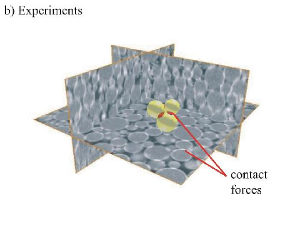
Figure 3: A novel fluorescence mechanism using confocal microscopy is providing new insight into the microstructure and the mechanics of jammed matter. The suitable model system is an emulsion comprised of oil droplets of approximately 3.4 $\mu$m dispersed in a refractive index matching solution. The system forms a random close packed structure by creaming or centrifugation giving rise to a force network. Based on the bright contact areas, the interdroplet forces can be extracted. The resulting micromechanics is being used to develop statistical theories of jammed materials.

2 Force distributions in a jammed emulsion

The micromechanics of jammed systems has been extensively studied in terms of the probability distribution of forces, $P(f)$. However, the experiments were previously confined to 2D granular packs [28, 47] or the measurement of the forces exerted at the walls of a 3D granular assembly [48, 49, 50, 51, 52] thus reducing the dimensionality of the problem. On the other hand, numerical simulations [53, 54, 52, 55] and statistical modelling [56] have provided the $P(f)$ for a variety of jammed systems, from structural glasses to foams and compressible particles, in 3D. Our novel experimental technique can be compared with all previous studies in search of a common behaviour. Apart from being the first study of $P(f)$ in the bulk, it is also the first study of jamming in an emulsion system.

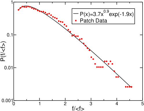
Figure 4: Probability distribution of the contact forces for the compressed emulsion system shown in Fig. 1b. We also show a fit to the theory developed in [43].

The result of the confocal images analysis, shown in Fig. 4, shows the probability distribution of interdroplet forces, $P(f)$, for the sample shown in Fig. 1b. We use a linear force model (see Section 1) to obtain the interdroplet forces from the contact area data extracted from the image analysis described above.

The distribution data shown are extracted from 1234 forces arising from 450 droplets. The forces are calculated from the bright, fluorescent patches that highlight the contact areas between the droplets as seen in Fig. 3. The droplets are only slightly deformed away from spherical at the low applied pressures. This indicates that the system is jammed near the RCP.

The data shows an exponential distribution at large forces, consistent with results of many previous experimental and simulation data on granular matter, foams, and glasses. The quantitative agreement between $P(f)$ of a variety of systems suggests a unifying microstructural behaviour governed by the jammed state. The salient feature of $P(f)$ in jammed systems is the exponential decay above the mean contact force. The behaviour in the low force regime indicates a small peak, although the power law decay tending towards zero is not well pronounced. The best fit to the data gives a functional form of the distribution (see Fig. 4):

$$P(f)\propto{f}^{0.9}e^{-1.9f/\bar{f}},$$ (2)

with $\bar{f}$ is the mean force. This form is consistent with the theoretical q-model [56] and with the model proposed in [43] which predicts a general distribution of the form $P(f)\propto f^{n}e^{-(n+1)f/\bar{f}}$, where the power law coefficient $n$ is determined by the packing geometry of the system and the coordination number.

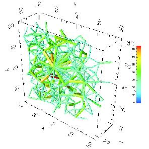
Figure 5: Force chains in emulsions: Plot of the interdroplet forces inside the packing of droplets obtained in the experiments. We plot only the forces larger than the average for better visualisation. Each rod joining the centers of two droplets in contact represents a force. The thickness and the colour of the rod is proportional to the magnitude of the force.

Our experimental data allows us to examine the spatial distribution of the forces in the compressed emulsion, shown in Fig. 5. In this sample volume, the forces appear to be uniformly distributed in space and do not show evidence of localisation of forces within the structure. Moreover, we find that the average stress is independent of direction, indicating isotropy. For comparison, we also show computer simulation results for isotropic packings of Hertz-Mindlin spherical particles in Fig. 6 (see Section 3) where force chains are not prominent either. On the other hand 2D packings clearly show the existence of force chains under isotropic pressure, indicating that their existence may be related to the dimensionality of the problem. Furthermore, force chains can be obtained in 3D by uniaxially compressing an isotropic packing, as shown in Fig. 6c. It should be noted that in the case of Fig. 6c an algorithm which looks for force chains is applied by starting from a sphere at the top of the system, and following the path of maximum contact force at every grain. Only the paths which percolate are plotted, i.e., the stress paths spanning the sample from the top to the bottom.

Interestingly, the salient feature of all the particulate packings shown in Figs. 5 and 6, irrespective of their spatial characteristics, is an exponential distribution of forces. This indicates that force chains are not necessary to obtain such a distribution. The rationalization of this observation has been exploited in the theory developed in [43] which is based on the assumption of uncorrelated force transmission through the packing.

(a)

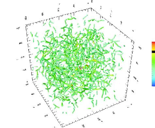
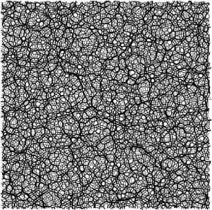
(b) (c)

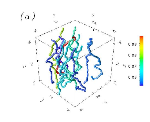
Figure 6: Force chains in granular matter. (a) Frictionless isotropic granular system at $p=100$ KPa in 3D from simulations. We plot only the forces larger than the average. Force chains are tenuous and not well defined. (b) Clearly visible force chains in a 2D frictional system from simulations. (c) Frictional system under uniaxial compression from simulations. Percolating force chains are seen in this case.

The mean coordination number of the system, $Z$, is another theoretically important parameter. It has been shown that the isostatic limit is achieved (in 3D) for $Z=4$ for frictional systems and $Z=6$ for smooth particles (see Section 1). This has not been tested in the real world until present, except in the famous experiment of Bernal for smooth particles who obtained a coordination number for spheres in contact of 6.4 for metallic balls of 1/8’ diameter. Even there, all particles in contact were counted, whereas the theory predicts the coordination number assuming only those particles which are exerting a force. Our experiments at low confining pressures (up to 200Pa) show that the mean coordination number is $Z\approx 6$ which can be interpreted as the isostatic limit for frictionless spheres.

This completes the study of the jammed structures in terms of the force distributions. There are more subtle ways in which the static structure of the configuration can be investigated as a statistical ensemble as we describe in the next section.

3 Experimental measurement of $\cal W$ and $X$

Having investigated the probability distribution of forces within the system, we now consider the distribution of the configurations of the packing. In Section 1 we have justified the application of statistical mechanics to jammed conditions, provided there is a mechanism for changing the configurations by tapping. The probability distribution of configurations is governed by Eq. (18).

Using an extension to the same image analysis method used to measure the distribution of forces, the 3D images of a densely packed particulate model system also allow for the characterisation of the volume function $\cal{W}$. This is performed by the partitioning of the images into first coordination shells of each particle, described in Section 1. The polyhedron obtained by such a partitioning is shown in Fig. 7 and its volume is calculated from Eq. (6).

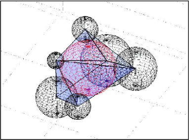
Figure 7: An example of a volume $\cal W$ as the polyhedron constructed from the 3D images. The centre grain (red) has 6 grains in contact (black), the centres of which are joined to form the polyhedron.

The ability to measure this function and therefore its fluctuations in a given particle ensemble, enables the calculations of the macroscopic variables. We calculate the probability distribution of the volume per particle in the whole image and find an exponential behaviour:

$$P({\cal W})\propto e^{-{\cal W}/\lambda X},$$ (3)

The exponential probability distribution of $\cal{W}$ enables the measurement of the compactivity $X$ according to Eq. (18). The value obtained in this way is $X=94\mu$m${}^{3}/\lambda$, shown in Fig. 8. The conversion of this measurement of the compactivity into a measurement of the analogue of temperature requires a new temperature scale for granular matter. In other words, $\lambda$ (the analogue of the Boltzmann constant in thermal systems) provides the link between volume fluctuations (energy) and compactivity (temperature) and needs to be determined for jammed matter.

We have shown that we can arrive at the thermodynamic system properties from the knowledge of the microstructure. Many images, i.e. configurations, can be treated in this way to test whether system size influences the macroscopic observables. If the particles are subjected to ultracentrifugation resulting in configurations of a higher density, the influence of pressure on the macroscopic variables can also be tested.

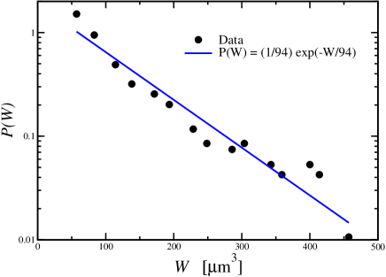
Figure 8: Probability distribution of $\cal W$ fitted with a single exponential. The decay constant is the compactivity, $X=94\mu m^{3}/\lambda$.

Such a characterisation of the governing macroscopic variables, arising from the information of the microstructure, allows one to predict the system’s behaviour through an equation of state. This is the first experimental study of such statistical concepts in particulate matter and opens new possibilities for testing the above described thermodynamic formulation. In principle, one can apply low amplitude vibrations to the system and observe the droplet configuration before and after the perturbation, thus testing the ideas proposed in the Boltzmann derivation.

Chapter 3 Jamming in a Periodic Box

The following section describes the potential for using computer simulations in testing the thermodynamic foundations raised in the previous sections. Rather than employing rough rigid grains for which most of the theoretical concepts have so far been devised, computer simulations are obliged to introduce some deformability into the constituent particles to facilitate the measurement of the particle interactions with respect to their positions. As a result, the entropic considerations which have been explained only in terms of the volume in the case of rigid grains in Section 1 will now be generalised to situations in which there is a finite energy of deformation in the system. The energy of the system will parametrise the compaction curves at varying confining pressures shown in Fig. 3.

The entropy Eq. (8) can then be redefined as a function of both energy and volume,

$$S(E,V)=\lambda\ln\Sigma_{\mbox{\scriptsize jammed}}(E,V).$$ (1)

The introduction of energy into the system implies a corresponding compactivity,

$$X_{E}^{-1}=\frac{{\partial S}}{{\partial E}},$$ (2)

where the subscript $E$ denotes that the compactivity is now the Lagrange multiplier controlling the energy of the jammed configuration, not the volume. Notice that $X_{E}$ differs from the temperature of an equilibrium system $T=\partial E/\partial S$ because the energy in Eq. (2) is the energy of the jammed configurations and not the thermal equilibrium energy. The assumptions of ergodicity and equally probable microstates for a given energy and volume are still valid here, just as they were for rigid grains in the previous sections.

The canonical distribution in Eq. (18) is generalised to

$$P_{\nu}=\frac{e^{(-E_{\nu}/\lambda X_{E}-{\cal W}_{\nu}/\lambda X_{V})}~{}~{}\Theta_{\nu}}{Z}.$$ (3)

The term $\Theta_{\nu}$ assures that we are considering only the jammed configuration. Its significance will be discussed in Section 2.

1 Simulating Jamming

In Section 2 we described the need for a true jammed configuration before any statistical measurement can be applied. While this process is achieved via external perturbations in a laboratory experiment, the equivalent procedure guaranteeing reproducible results using simulations, requires a particular ‘equilibration’ procedure. At each pressure, the grains are pretreated in the following way in order to ensure that all memory effects have been lost in the system.

We perform Molecular Dynamics (MD) simulations of an assembly of spherical grains in a periodically repeated cubic cell. The system is composed of soft elasto-frictional spherical grains interacting via Hertz-Mindlin contact forces, Coulomb friction and viscous dissipative terms. Two model systems are investigated: granular materials and compressed emulsions.

Granular matter model.– Particles are modelled as viscoelastic spheres with different coefficients of friction. Interparticle forces are computed using the principles of contact mechanics [57]. Full details are given in Refs. [52, 58, 17]. The normal force $F_{n}$ has the typical 3/2 power law dependence on the overlap between two spheres in contact (Hertz force), while the transverse force $F_{t}$ depends linearly on the shear displacement between the spheres, as well as on the value of the normal displacement (Mindlin tangential elastic force). As the shear displacement increases, the elastic tangential force $F_{t}$ reaches its limiting value given by Amonton’s law for no adhesion, $F_{t}\leq\mu_{f}F_{n}$, which is a special case of Coulomb’s law. Viscous dissipative forces, proportional to the relative normal and tangential velocities of the particles, are also included to allow the system to equilibrate.

A granular system with tangential elastic forces is path-dependent since the work done in deforming the system depends upon the path taken and not just the final state. On the other hand, a system of spheres interacting only via normal forces is said to be path-independent, and the work does not depend on the way the strain is applied. It turns out that this is a good model for a compressed emulsion system since they do not exhibit frictional forces.

Compressed emulsions model.– A system of frictionless viscoelastic spherical particles could be thought of as a model of compressed emulsions [59, 60], see also [42] for details. Even though they can be modelled in this way, an important difference arises in the interdroplet forces, which are not given in terms of the bulk elasticity, as they are in the Hertz theory. Instead, forces are given by the principles of interfacial mechanics [44]. For small deformations with respect to the droplet surface area, the energy of the applied stress is presumed to be stored in the deformation of the surface. The simplest approximation considers an energy of deformation which is quadratic in the area of deformation [44], analogous to a harmonic oscillator potential which describes a spring satisfying Hooke’s law.

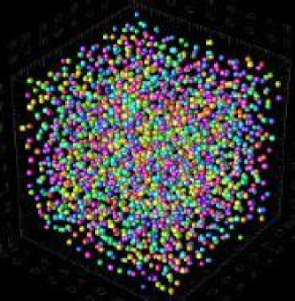
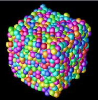
Figure 1: Preparation protocol for granular materials and droplets. We start with a system of noninteracting spheres (a) and then we apply a compression protocol to reach the jammed state (b)

There have been several more detailed numerical simulations [59] to improve on this model and allow for anharmonicity in the droplet response by also taking into consideration the number of contacts by which the droplet is confined. Typically these improved models lead to a force law for small deformations of the form $F_{n}\propto A^{b}$ , where $A$ is the area of deformation and $b$ is a coordination number dependent exponent ranging from 1 (linear model) to 3/2 (Hertz model). For simplicity and for a better comparison with the physics of granular materials, in the following we will show results only considering the nonlinear 3/2 dependence of the normal force. A more realistic nonlinear dependence is considered elsewhere in [61].

Thus we adjust the MD model of granular materials to describe the system of compressed emulsions by only excluding the transversal forces (tangential elasticity and Coulomb friction). The continuous liquid phase is modelled in its simplest form, as a viscous drag force acting on every droplet, proportional to its velocity.

Preparation protocol.— Our aim is to introduce a numerical protocol designed to mimic the experimental procedure used to achieve the jammed state, as explained in Section 2. The simulations begin with a gas of noninteracting grains distributed at random positions in a periodically repeated cubic cell, depicted in Fig. 1, showing snapshots of our typical simulations with 10,000 particles of size $R=100\mu$m. To avoid issues of path-dependency introduced by the shear forces, the transverse force between the grains is excluded from the calculation ($F_{t}=0$). Because there are no transverse forces, the grains slip without resistance and the system reaches the high volume fractions found experimentally, thus avoiding the irreversible branch of the compaction curve. This procedure essentially mimics the path to jammed states for the compressed emulsion system.

The protocol is then repeated for grains with friction. Initially, a fast compression of the grains brings the system to the irreversible branch of the compaction curve. It is then necessary to apply a compression protocol in order to reach a target pressure. This pressure is maintained with a “servo” mechanism by the continuous application of an oscillatory strain until the system reaches the jammed state [62]. The servo mechanism is analogous to the application of a small tapping amplitude to reach the reversible branch of the compaction curve, Fig. 2. In general, we find that by preparing the system with frictional and elastic tangential forces, the system reaches states of lower volume fractions. At the end of the preparation protocol (depicted by the dashed lines in Fig. 2a) we obtain a set of jammed systems at different stresses (for granular materials) or osmotic pressures (for droplets) [52].

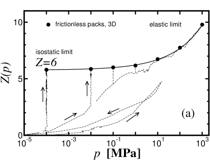
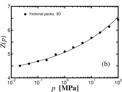
Figure 2: Coordination number versus pressure. (a) Frictionless packs in 3D ($\mu=0$). The system is isostatic $Z_{c}=2D=6$ as $p\to 0$. (b) Frictional packs in 3D (finite $\mu$).

1 Isostatic jamming

Consider a static packing of grains under an external force ${\rm\bf f}^{\mbox{\scriptsize ext}}$. The internal stresses obey the Cauchy equations:

$$\partial_{i}\sigma_{ij}+f_{j}^{\mbox{\scriptsize ext}}=0.$$ (4)

Since there are 3 equations (in 3-D) for 6 independent stress components (the stress tensor is symmetric), then the system is indeterminate, and the Cauchy equations must be augmented by additional constitutive equations. The conventional elastic approach is then to consider the deformability of the packing which is described by the strain field. Linear constitutive relations are introduced to relate the strain to the stress via the elastic constants of the material (Hooke’s law). For an isotropic elastic body only two elastic constants (for instance, the shear modulus and the Poisson ratio) are sufficient to fully describe the stress transmission in an elastic packing [63].

In the limit of infinitely rigid grains the strain field is ill-defined and the validity of elasticity theory is open to debate. In this case, it has been argued that it is possible to solve the stress distribution, based on Newton’s equations alone without resorting to the existence of the strain, only when the system is at a particular minimal coordination number [64, 23, 38]. The granular indeterminacy is then solved by resorting to the configurational information alone. Such approaches are intimately related to the thermodynamics of jamming [39].

The minimal coordination number can be understood in terms of simple constraint arguments for a system of $N$ rigid spherical grains in $D$ dimensions [65, 66, 64]. In the case of frictionless grains, $ZN/2$ normal forces have to be determined with $DN$ equations of force balance. The critical coordination number for which the equations of force balance are soluble is fount to be $Z_{c}=2D$. Similar arguments lead to a minimal coordination of $Z_{c}=D+1$ for infinitely rough spherical grains, i.e. grains with finite tangential forces, $F_{t}$, but with an infinitely large friction coefficient ($\mu\to\infty$).

Below $Z_{c}$ the system cannot be jammed and it exists only in suspensions. Above $Z_{c}$ the system is underconstrained and elasticity theory may give the correct approach to describe such a packing of deformable grains. At the minimal coordination number the system is in a state of marginal rigidity [38], otherwise known as the isostatic limit [65, 66].

In order to test the existence of the isostatic limit we study the coordination number dependence on pressure for the two cases: frictionless grains and those with friction. The preparation protocols explained above are performed to achieve different target pressures and we obtain the average coordination number $Z(p)$ of the jammed states as a function of the pressure, as shown in Fig. 2.

In the case of frictionless grains we find that the coordination number of the pack approaches the minimal value $Z_{c}\approx 6$ as $p\to 0$. At low pressures compared to the shear modulus of the beads ($p\ll 26$ GPa) the system behaves most like a pack of rigid balls, thus approaching the isostatic limit. The same preparation protocol gives $Z_{c}\approx 4$ in 2D confirming the $Z_{c}=2D$ relationship (results not shown here). The preparation protocol for grains with infinite friction in 3D gives rise to different packings with lower coordination numbers. Our results suggest that the isostatic limit $Z_{c}=4$ is achieved for infinitely rough grains as $p\to 0$ [61]. Grains with finite friction also seem to tend to the minimal coordination number $Z_{c}\approx 4$ as seen in Fig. 2b, but at much smaller pressures than those achieved in our calculations. Therefore, it is difficult to draw conclusions as to whether the isostatic limit requires even lower confining pressures or not. In fact, recent computational studies have suggested that the isostatic limit may not exist in packs with finite friction [67]. However, this study uses a different compression protocol more akin to a fast quench, which may leave the system trapped in the irreversible branch of the compaction curve due to the system’s inability to explore all the available configurational space.

The approach to the marginal rigidity state $Z\to Z_{c}$ can be seen as a jamming transition between a solid-like state with a finite shear modulus and a liquid-like state with no resistance to shear, observed in suspensions. In fact we find that the stress $\sigma$ and the shear modulus $G$ of the packing vanish according to a power law as the system approaches a critical density, $\phi_{c}$, corresponding to the jamming transition [52]:

$$\sigma\sim(\phi-\phi_{c})^{\alpha},~{}~{}~{}~{}~{}~{}~{}~{}G\sim(\phi-\phi_{c})^{\beta}.$$ (5)

The exponents $\alpha$, $\beta$ can easily be calculated in terms of the microscopic law of interparticle interactions. For instance, Hertz theory predicts the values of $\alpha=3/2$ and $\beta=1/2$, in agreement with with our simulation results. The critical density $\phi_{c}$ depends on the interaction potential between the grains. A value $\phi_{c}=0.63\approx\phi_{\mbox{\scriptsize RCP}}$ is achieved for frictionless grains and corresponds to the volume fraction at RCP [40]. On the other hand $\phi_{c}<\phi_{\mbox{\scriptsize RCP}}$ are achieved for grains with friction. These states correspond to RLPs. The jamming transition can be thought of as a particular second-order phase transition because the exponents are not universal; they depend on the details of the microscopic interactions between the grains [68].

The coordination number also approaches the critical minimal value as a power law. Empirically, we find (Fig. 2)

$$Z(p)=Z_{c}+\left(\frac{p}{~{}\mbox{6.45 MPa}}\right)^{1/3}.$$ (6)

with $Z_{c}=6$ and $Z_{c}=4$ for the infinitely smooth and infinitely rough grains, respectively.

After having characterised the jammed state, the computational study proceeds to develop the thermodynamics using the states depicted in Fig. 2 as the starting point.

2 Testing the Thermodynamics

If it were true that a thermodynamic framework could describe the behavior of jammed systems, it stands to reason that the compactivity $X_{E}$ of the granular pack can be measured from a dynamical experiment involving the exploration of the energy landscape. We examine the validity of this statement with computer simulations in the following discussion.

Following the equilibration procedure, the exploration of the energy landscape equivalently needs a driving mechanism such that all appropriate configurations are sampled. This is achieved via a slow shearing procedure which has for an aim to probe each static configuration by allowing the system to evolve at a very slow shear rate. We first introduce a procedure to obtain a dynamical measurement of the compactivity via a diffusion-mobility protocol. We call this quantity the effective temperature $T_{\mbox{\scriptsize eff}}$ and show that it satisfies a form of the zero-th law of thermodynamics and thus has a thermodynamic meaning.

The next crucial test for this assumption is to show that the effective temperature obtained dynamically can also be obtained via a flat average over the jammed configurations. Such a test has been performed in [17], where it was indeed shown that $T_{\mbox{\scriptsize eff}}$ is very close to the compactivity of the packing $X_{E}$. This result will be shown explicitly in Section 2. We conclude that the jammed configurations explored during shear are sampled in an equiprobable way as required by the ergodic principle. Moreover the dynamical measurement of compactivity renders the thermodynamic approach amenable to experimental investigations.

In the next sections we calculate the effective temperature of the packing dynamically and show its relation to the compactivity, calculated employing a configurational average.

1 Exploring the jammed configurations dynamically: effective temperature $T_{\mbox{\scriptsize eff}}$

Consider a ‘tracer’ body of arbitrary shape immersed in a liquid in thermal equilibrium. As a consequence of the irregular bombardment by the particles of the surrounding liquid, the tracer performs a diffusive, fluctuating ‘Brownian’ motion. The motion is unbiased, and for large times the average square of the displacement goes as $\langle|x(t)-x(0)|^{2}\rangle=2Dt$, where $D$ is the diffusivity. On the other hand, if we pull gently on the tracer with a constant force $F$, the liquid responds with a viscous, dissipative force. The averaged displacement after a large time is $\langle[x(t)-x(0)]\rangle=F\chi t$, where $\chi$ is the mobility. Although both $D$ and $\chi$ strongly depend on the shape and size of the tracer, they turn out to always be related by the Einstein relation

$$T=D/\chi,$$ (7)

(a form of the Fluctuation-Dissipation Theorem, FDT), where $T$ is the temperature of the liquid.

The Einstein relation is strictly valid for equilibrium thermal systems. However, it has been shown that fluctuation-dissipation relations are relevant to describe the thermodynamics of out-of-equilibrium systems. Insight into the validity of fluctuation-dissipation relations to describe far from equilibrium systems first came from glass theory [10, 11]. Recent analytic schemes for glasses have shown that a generalized FDT gives rise to a well-defined effective temperature which is different from the bath temperature [12]. It governs the heat flow and the slow components of fluctuations and responses of all observables. Explicit verifications of this approach have been made until present within the mean-field/mode-coupling models of the glass transition [13]. More recent studies have supported the existence of effective temperatures in schematic finite-dimensional models of glassy systems [15, 16].

The existence of a similar effective temperature for out-of-equilibrium sheared granular systems is by no means obvious. Moreover, its existence may provide a profound link between the physics of granular materials and glasses. In the absence of a first principle derivation, one needs to ascertain its validity for every particular case experimentally, or numerically at the least. In order to test the existence of an effective temperature with a thermodynamic meaning for dense slow-moving granular matter we perform a numerical study of a diffusion-mobility computation in conditions that can be reproduced in the laboratory [17].

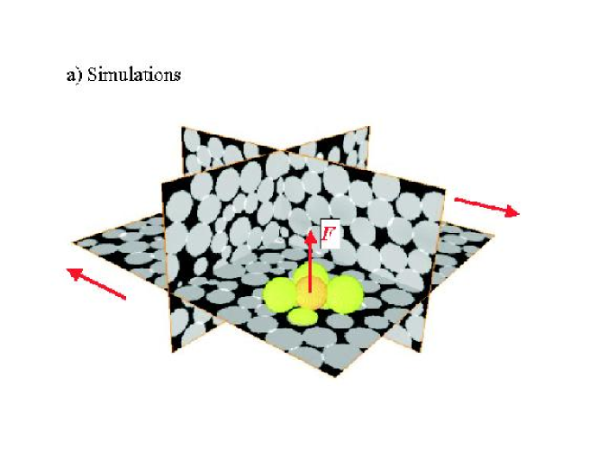
Figure 3: Simulations of grains of 100 microns interacting via Hertz-Mindlin contact forces. A slow shear flow, indicated by the arrows, is applied to the jammed system. We follow the tracer particle trajectories to obtain the diffusivity. An external force $F$ is then applied to the tracers in response to which we measure the particle mobility. These dynamical measurements yield an ”effective temperature” obtained from an Einstein relation which is indeed very close to the compactivity obtained by a flat average over the ensemble of jammed configurations.

We consider a system of large and small spherical grains in a periodic cell. The simulations involve the application of a gentle shear on the particles in the $y$-$z$ plane, at constant volume (see Fig. 3). The shearing mechanism moves the periodic images at the top and the bottom of the cell with velocities $\dot{\gamma}L/2$, where $\dot{\gamma}$ is the shear rate (Lees-Edwards boundary conditions [69]). A linear, uniform velocity profile along the $z-$direction is obtained using a modified set of equations to suit our computations (see Chapter 8 of [69]). Periodic boundary conditions are enforced in the $x-$direction and the $y-$direction of the flow. We focus our study on the region of slow shear rates, where the system is always close to jamming. We avoid shear bands by imposing a linear velocity profile and avoid segregation which may occur at much longer time scales than those employed in our computations.

The time resolved displacement of the particles are measured to obtain their random fluctuations as well as the response function of the tracers to allow the determination of the effective temperatures via the Einstein relation (7). We measure the spontaneous fluctuations $\langle|x(t)-x(0)|^{2}\rangle$ and force-induced displacements $\langle[x(t)-x(0)]\rangle/F$, where $F$ is a small external force in the $x$-direction, for two types of tracers with different sizes. We calculate $T_{\mbox{\scriptsize eff}}$ by using parametric plots of $\langle|x(t)-x(0)|^{2}\rangle$ versus $\langle[x(t)-x(0)]\rangle/F$ with $t$ as parameter. The parametric procedure of obtaining the effective temperatures allows the study of $T_{\mbox{\scriptsize eff}}$ for different time scales [12, 16]. Hence we determine the temperature of the different modes of relaxation (see also [70, 71]).

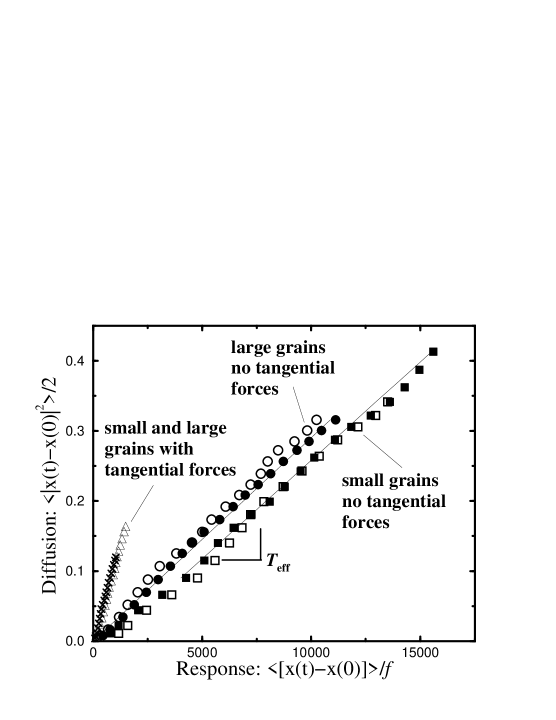
Figure 4: Parametric plot of diffusion vs response function for small and large grains and for spheres interacting with tangential forces (grains) and without tangential forces (emulsions). The fitting at long time scales shows the existence of a well-defined temperature which is the same for small and large grains: $T_{\mbox{\scriptsize eff}}=2.8\times 10^{-5}$ for grains without transverse forces and $T_{\mbox{\scriptsize eff}}=1.2\times 10^{-4}$ for grains with Mindlin transverse forces and Coulomb friction. These effective temperatures (measured here in reduced units [17]) are in fact very large, i.e. $\sim 10^{14}$ times $k_{B}T$ at room temperature, as expected. We calculate the response function for several small external fields and find the same temperature indicating that we are in the linear response regime. Plotted are results for a system without transverse forces using: $F=1.7\times 10^{-5}$ (small grains $\Box$, large grains $\circ$) and $F=2.6\times 10^{-5}$ (small grains  , large grains $\bullet$). For a system with tangential forces and Coulomb friction we show the case $F=6\times 10^{-5}$ (small grains $\bigtriangleup$, large grains $\times$).

Our data is consistent with a granular Einstein relation (Fig. 4):

$$\langle|x(t)-x(0)|^{2}\rangle=2~{}T_{\mbox{\scriptsize eff}}\frac{\langle[x(t)-x(0)]\rangle}{F},$$ (8)

valid for all tracers with the same fluctuation-dissipation temperature $T_{\mbox{\scriptsize eff}}$ for widely separated time scales.

If there is an underlying thermodynamics, it will impose that the effective temperature be independent of the tracer’s size: a strong condition required for the thermodynamic hypothesis. We then verify if all tracers have “equilibrated” at the same effective temperature by calculating the effective temperature for small and large tracers and finding that indeed they are the same. Figure 4 shows the parametric plot of the diffusion versus response function for systems with friction and frictionless grains. In both cases we consider the temperature of the small and large grains and obtain the same temperature. The fact that the effective temperature is the same for both types of particles and that it is only valid for the long-time relaxation suggest that $T_{\mbox{\scriptsize eff}}$ can be considered to be the temperature of the slow modes.

2 Exploring the jammed configurations via a flat average. Test of ergodicity: $T_{\mbox{\scriptsize eff}}=X_{E}$

The systems under investigation have exponentially large (in the number of particles) number of stable states jammed at zero bath temperature. In the previous section we explored such an energy landscape via slow shear. Next, we develop an independent method to study the configurational space. It allows us to investigate the statistical properties of the jammed states available at a given energy and volume. In turn we investigate whether it is possible to relate the dynamical temperature obtained above via a diffusion-mobility protocol to the configurational compactivity based on jammed states.

In order to calculate $X_{\mbox{\scriptsize E}}$ and compare with the obtained $T_{\mbox{\scriptsize eff}}$ we need to sample the jammed configurations at a given energy and volume in a equiprobable way. In order to do this we sample the jammed configurations with the following probability distribution:

$$P_{\nu}\sim\exp[-E^{\nu}/T^{*}-E^{\nu}_{\mbox{\scriptsize jammed}}/T_{\mbox{\scriptsize aux}}]$$ (9)

Here the deformation energy $E$ corresponds to the Hertzian energy of deformation of the grains or the Princen energy for droplets. The extra term added in Eq. (9) allows us to perform the flat sampling of the jammed states and plays the role of the term $\Theta_{\nu}$ in Eq. (3). The jammed energy is such that it vanishes at the jammed configurations:

$$E_{\mbox{\scriptsize jammed}}\propto\sum_{a}\left|{\rm\bf F}_{a}\right|^{2},$$ (10)

where ${\rm\bf F}_{a}$ is the total force exerted on particle $a$ by its neighbours.

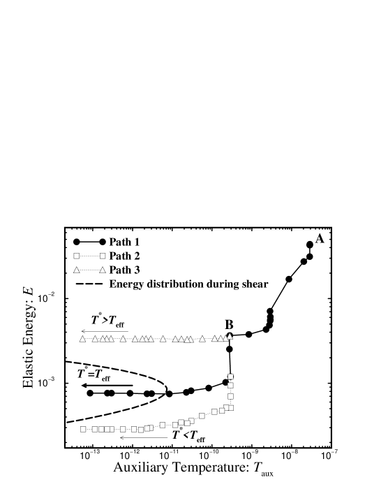
Figure 5: Annealing procedure to calculate $X_{E}$ at different elastic compressional energies. We plot the elastic energy vs $T_{\mbox{\scriptsize aux}}$ during annealing together with the distribution of elastic energies obtained during shear (dashed curve, mean value $\langle E\rangle=8.4\times 10^{-4}$). We equilibrate the system for $40\times 10^{6}$ iterations at A: $(T^{*}=3.4\times 10^{-2},T_{\mbox{\scriptsize aux}}=3\times 10^{-8})$. We then anneal slowly both temperatures until B: $(T^{*}=3.4\times 10^{-4},T_{\mbox{\scriptsize aux}}=3\times 10^{-10})$, where we split the trajectory in three paths in the $(T^{*},T_{\mbox{\scriptsize aux}})$ plane. Path 1: we anneal $T_{\mbox{\scriptsize aux}}\to 0$ and $T^{*}\to 2.8\times 10^{-5}$ which corresponds to $T_{\mbox{\scriptsize eff}}$ obtained during shear (Fig. 4). Path 2: we anneal $T_{\mbox{\scriptsize aux}}\to 0$ and $T^{*}\to 3.4\times 10^{-6}$. Path 3: we anneal $T_{\mbox{\scriptsize aux}}\to 0$ but keep $T^{*}=3.4\times 10^{-4}$ constant. When we set $T^{*}=T_{\mbox{\scriptsize eff}}$ (Path 1), the final elastic compressional energy value when $T_{\mbox{\scriptsize aux}}\to 0$ falls inside the distribution of energies obtained, and it is very close to the mean value of the elastic energy during shear $\langle E\rangle$. This proves that $T_{\mbox{\scriptsize eff}}=X_{E}$ under the numerical accuracy of the simulations. For other values of $T^{*}\neq T_{\mbox{\scriptsize eff}}$ the final $E$ falls out of the distribution obtained during shear (Paths 2 and 3). We also follow different trajectories (not shown in the figure) to $T^{*}\to 2.8\times 10^{-5},T_{\mbox{\scriptsize aux}}\to 0$ and find the same results indicating that our procedure is independent of the annealing path.

We introduce two “bath” temperatures (these temperatures are $\sim 10^{14}$ times the room temperature) which will allow us to explore the configuration space and calculate the entropy of the packing assuming a flat average over the jammed configurations. We perform equilibrium MD simulations with two auxiliary “bath” temperatures $(T^{*},T_{\mbox{\scriptsize aux}})$, corresponding to the partition function (9). Annealing $T_{\mbox{\scriptsize aux}}$ to zero selects the jammed configurations ($E_{\mbox{\scriptsize jammed}}=0$), while $T^{*}$ fixes the energy $E$.

In practice we perform equilibrium MD simulations with a modified potential energy:

$$U=\frac{T_{\mbox{\scriptsize aux}}}{T^{*}}E+E_{\mbox{\scriptsize jammed}},$$ (11)

and calculate the force on each particle from ${\rm\bf F}=-{\rm\bf\nabla}U$. Since we need to calculate the force from a potential energy, only conservative systems can be studied with this method. Thus we focus our calculations on the system of frictionless particles. The auxiliary temperature $T_{\mbox{\scriptsize aux}}$ is controlled by a thermostat which adjusts the velocities of the particles to a kinetic energy determined by $T_{\mbox{\scriptsize aux}}$. We start by equilibrating the system at high temperatures ($T_{\mbox{\scriptsize aux}}$ and $T^{*}$ $\sim\infty$) and anneal slowly the value $T_{\mbox{\scriptsize aux}}$ to zero and tune $T^{*}$ so as to reach the value of $E$ that corresponds to the average deformation energy obtained during shear.

The partition function is

$$Z=\sum_{\nu}\exp[-E^{\nu}/T^{*}-E^{\nu}_{\mbox{\scriptsize jammed}}/T_{\mbox{\scriptsize aux}}],$$ (12)

from where we obtain the compactivity as

$$T^{*}=\frac{\partial E}{\partial S}\stackrel{{\scriptstyle\mbox{\scriptsize$T_{\mbox{\scriptsize aux}}\to 0$}}}{{\longrightarrow}}X_{E},$$ (13)

Thus at the end of the annealing process ($T_{\mbox{\scriptsize aux}}\to 0$), $T^{*}(E)=X_{E}(E)$, since in this limit we are sampling the configurations with vanishing fraction of moving particles at a given $E$.

At the end of the protocol the compactivity at a given deformation energy can be obtained as illustrated in Fig. 5. The remarkably result is that the compactivity and the effective temperature obtained dynamically are found to coincide to within the computational error [17],

$$X_{E}\approx T_{\mbox{\scriptsize eff}}.$$ (14)

This provides strong evidence for the validity of the effective temperature as a dynamical estimate of the compactivity, and more importantly, justifies the use of the novel statistical measurements we have presented in fully characterising the macroscopic properties of the system.

To summarise, the fact that slow relaxation modes can be characterized by a temperature raises the question of the existence of a form of ergodicity for the structural motion, allowing a construction of a statistical mechanics ensemble for the slow motion of the grains. This argument leads us back to the ideas of the thermodynamics of jammed states. In parallel to these dynamical measurements, the same information is drawn from the system by a flat statistical average over the jammed configurations. Once all the static configurations have been visited by the system, the compactivity $X_{E}$ can be calculated from the statistics of the canonical ensemble of the jammed states. The logarithm of the available configurations at a given energy and volume reveals the entropy, from which the compactivity is calculated. Our explicit computation shows that the temperature arising from the Einstein relation (8) can be understood in terms of the configurational compactivity $X_{E}$ arising from the statistical ensemble of jammed states. This provides a strong evidence for the validity of the thermodynamic approach.

References

- [1] A. Liu and S. R. Nagel, (eds.), Jamming and Rheology: Constrained Dynamics on Microscopic and Macroscopic Scales, Taylor & Francis, London, 2001.
- [2] P. G. Debenedetti and F. H. Stillinger, Nature 410, 259 (2001).
- [3] M. Goldstein, J. Chem. Phys. 51, 3728 (1969).
- [4] F. H. Stillinger and T. A. Weber, Phys. Rev. A 25, 978 (1982); ibid, Science 225, 983 (1984).
- [5] S. Sastry, P. G. Debenedetti, and F. H. Stillinger, Nature 393, 554 (1998).
- [6] W. Kob, F. Sciortino, and P. Tartaglia, Europhys. Lett. 49, 590 (2000).
- [7] B. Coluzzi, G. Parisi, and P. Verrocchio, Phys. Rev. Lett. 84, 306 (2000).
- [8] A. Fierro, M. Nicodemi, and A. Coniglio, Europhys. Lett. 59, 642 (2002).
- [9] L. C. E. Struik, Physical Aging in Amorphous Polymers and other Materials, (Elsevier, Houston, 1978)
- [10] M. Mézard, G. Parisi and M. A. Virasoro, Spin Glass Theory and Beyond (World Scientific, Singapore, 1987).
- [11] T. R. Kirkpatrick and D. Thirumalai, Phys. Rev. B 36, 5388 (1987); T. R. Kirkpatrick and P. Wolynes, Phys. Rev. A 35, 3072 (1987).
- [12] L. F. Cugliandolo, J. Kurchan, and L. Peliti, Phys. Rev. E 55, 3898 (1997).
- [13] J. Kurchan, Rheology and how to stop aging, in A. Liu and S. R. Nagel, (eds.), Jamming and Rheology: Constrained Dynamics on Microscopic and Macroscopic Scales, Taylor & Francis, London, 2001, cond-mat/9812347.
- [14] J. Kurchan, J. Phys. Condensed Matter 29, 6611 (2000).
- [15] M. Nicodemi, Phys. Rev. Lett. 82, 3734-3737 (1999).
- [16] A. Barrat, J. Kurchan, V. Loreto, and M. Sellitto Phys. Rev. Lett. 85, 5034 (2000); ibid Phys. Rev. E 63, 51301 (2001).
- [17] H. A. Makse and J. Kurchan, Nature 415, 614 (2002).
- [18] S. F. Edwards, The aging of glass forming liquids, in Disorder in Condensed Matter Physics (eds J. Blackman, & J. Taguena) 147-154 (Oxford University Press, Oxford, 1991).
- [19] S. F. Edwards, The role of entropy in the specification of a powder, in Granular matter: an interdisciplinary approach (ed A. Mehta) 121-140 (Springer-Verlag, New York, 1994).
- [20] S. F. Edwards and R. B. S. Oakeshott, Physica A 157, 1080 (1989).
- [21] A. Mehta, and S. F. Edwards, Physica A 157, 1091 (1989).
- [22] J. Brujić, S. F. Edwards, and D. Grinev, Phil. Trans. R. Soc. Lond. A, 361, 741 (2003).
- [23] J.-P. Bouchaud, M. E. Cates, and P. Claudin, J. Phys. I (France) 5, 639 (1995); M. E. Cates, P. Wittmer, J.-P. Bouchaud, and P. Claudin, Phys. Rev. Lett. 81, 1841 (1998).
- [24] J. B. Knight, E. E. Ehrichs, V. Yu. Kuperman, J. K. Flint, H. M. Jaeger, and S. R. Nagel, Phys. Rev. E54, 5726 (1996).
- [25] S. B. Savage, Adv. Appl. Mech. 24, 289 (1994).
- [26] J. T. Jenkins, and S. B. Savage, J. Fluid Mech. 130, 187 (1983).
- [27] J.J. Alonso and H.J. Herrmann, Phys. Rev. Lett. 76, 4911 (1996).
- [28] R. P. Behringer and J. T. Jenkins, eds., Powders & Grains 97 (Balkexma, Rotterdam, 1997).
- [29] E. R. Nowak, J. B. Knight, M. L. Povinelli, H. M. Jaeger and S. R. Nagel. Powder Technol. 94, 79 (1997).
- [30] E. R. Nowak, J. B. Knight, E. BenNaim, H. M. Jaeger and S. R. Nagel, Phys. Rev. E 57, 1971 (1998).
- [31] P. Philippe, and D. Bideau, Europhys. Lett. 60, 677 (2002).
- [32] J. Brujić, P. Wang, D. L. Johnson, O. Sindt, and H. A. Makse (SDR report, to be published).
- [33] A. Chakravarty, S. F. Edwards, D. V. Grinev, M. Mann, T. E. Phillipson, A. J. Walton, Proceedings of the Workshop on Quasi-static Deformations of Particulate Materials, to be published.
- [34] A. J. Liu and S. R. Nagel, Nature 396, 21 (1998).
- [35] V. Trappe, V. Prasad, L. Cipelletti, P. N. Segre, and D. A. Weitz, Nature 411, 772 (2001).
- [36] G. D’Anna and G. Gremaud, Nature 413, 407 (2001).
- [37] L. D. Landau and E. M. Lifshitz, Statistical Physics (Pergamon, NY, 1970).
- [38] R. C. Ball and R. Blumenfeld, Phys. Rev. Lett. 88, 115505 (2002).
- [39] R. Blumenfeld and S. F. Edwards, Phys. Rev. Lett. 90, 114303 (2002).
- [40] J. D. Bernal, and J. Mason, Nature 188, 910 (1960); J. D. Bernal, Proc. Roy. Soc. London, Ser. A 280, 299 (1964).
- [41] G. D. Scott, Nature 188, 908 (1960).
- [42] J. Brujić, S. F. Edwards, D. V. Grinev, I. Hopkinson, D. Brujić, and H. A. Makse, Faraday Discuss., 123, 207 (2003).
- [43] J. Brujić, S. F. Edwards, I. Hopkinson, and H. A. Makse, Physica A 327, 201 (2003).
- [44] H. M. Princen, J. Colloid Interface Sci. 91, 160 (1983).
- [45] T. G. Mason, J. Bibette, and D. A. Weitz, Phys. Rev. Lett. 75, 2051 (1995).
- [46] S. F. Edwards, J. Brujić, and H. A. Makse, A basis for the statistical mechanics of granular systems. Submitted to Physica A, 2003.
- [47] G. W. Baxter, in Powders & Grains 97 (R. P. Behringer and J. T. Jenkins, eds.) (Balkexma, Rotterdam, 1997).
- [48] C.-H. Liu, S. R. Nagel, D. A. Schecter, S. N. Coppersmith, S. N. Majumdar, O. Narayan, and T. A. Witten, Science 269, 513 (1995).
- [49] D. M. Mueth, H. M. Jaeger and S. R. Nagel, Phys. Rev. E, 57, 3164 (1998).
- [50] G. Lovoll, K. N. Maloy and E. G. Flekkoy, Phys. Rev. E 57, 5872 (1999).
- [51] D. L. Blair, N. W. Mueggenburg, A. H. Marshall, H. M. Jaeger, and S. R. Nagel, Phys. Rev. E 63, 041304 (2001).
- [52] H. A. Makse, D. L. Johnson, and L. M. Schwartz, Phys. Rev. Lett. 84, 4160 (2000).
- [53] F. Radjai, M. Jean, J. Moreau, and S. Roux, Phys. Rev. Lett. 77, 274 (1996).
- [54] C. Thornton, KONA Powder and Particle 15, 81 (1997).
- [55] C. S. O’Hern, S. A. Langer, A. J. Liu, and S. R. Nagel, Phys Rev. Lett. 86, 111 (2001).
- [56] S. N. Coppersmith, C.-H. Liu, S. Majumdar, O. Narayan and T. A. Witten, Phys. Rev. E 53, 4673 (1995).
- [57] K. L. Johnson, Contact Mechanics, (Cambridge University Press, Cambridge, 1985).
- [58] H. A. Makse, N. Gland, D. L. Johnson, and L. M. Schwartz, Phys. Rev. Lett. 83, 5070 (1999).
- [59] M.-D. Lacasse, G. S. Grest, D. Levine, T. G. Mason, and D. A. Weitz, Phys. Rev. Lett. 76, 3448 (1996).
- [60] D. J. Durian, Phys. Rev. Lett. 75, 4780 (1995).
- [61] H. Zhang, N. Gland, and H. A. Makse (preprint).
- [62] P. A. Cundall and O. D. L. Strack, Géotechnique 29, 47 (1979).
- [63] L. D. Landau and E. M. Lifshitz, Theory of Elasticity (Pergamon, NY, 1970).
- [64] S. F. Edwards and D. V. Grinev, Phys. Rev. Lett. 82, 5397 (1999).
- [65] S. Alexander, Phys. Rep. 296, 65 (1998).
- [66] C. F. Moukarzel, Phys. Rev. Lett. 81, 1634 (1998).
- [67] L. E. Silbert, D. Ertas, G. S. Grest, T. C. Halsey, and D. Levine, Phys. Rev. E 65, 031304 (2002).
- [68] C. S. O’Hern, S. A. Langer, A. J. Liu, and S. R. Nagel, Phys. Rev. Lett. 88, 075507 (2002).
- [69] M. P. Allen and D. J. Tildesley, Computer Simulations of Liquids (Clarendon Press, Oxford, 1987).
- [70] I. K. Ono, C. S. O’Hern, D. J. Durian, S. A. Langer, A. J. Liu, and S. R. Nagel, Phys. Rev. Lett. 89, 095703 (2002).
- [71] S. A. Langer and A. J. Liu, Europhysics Lett. 49, 68 (2000).