Quantum Dynamics of a Nanomagnet in a Rotating Field.

Abstract

Quantum dynamics of a two-state spin system in a rotating magnetic field has been studied. Analytical and numerical results for the transition probability have been obtained along the lines of the Landau-Zener-Stueckelberg theory. The effect of various kinds of noise on the evolution of the system has been analyzed.

I Introduction

Molecular magnets with high spin and high magnetic anisotropy can be prepared in long-living excited quantum states by simply applying a magnetic field Sessoli . In a time dependent magnetic field, they exhibit stepwise magnetic hysteresis due to resonant quantum tunneling between spin levels Friedman . This phenomenon has been intensively studied theoretically within models employing Landau-Zener-Stueckelberg (LZS) effect Landau ; Zener ; Stueckelberg . The formulation of the problem, independently studied by Landau Landau , Zener Zener , and Stueckelberg Stueckelberg at the inception of quantum theory is this. Consider a system characterized by quantum states $|1\rangle$ and $|2\rangle$ with energies $E_{1}$ and $E_{2}$ respectively. Let the system be initially prepared in the lower-energy state, $|1\rangle$, and the field be changing such (due to, e.g., Zeeman interaction of the magnetic field with a spin) that $E_{1}$ is shifting up while $E_{2}$ is shifting down. After the levels cross and the distance between them continues to increase, the system, with LZS probability, $P=\exp(-\pi\Delta^{2}/2\hbar v)$, remains in the state $|1\rangle$. Here ${\Delta}$ is the tunnel splitting of $|1\rangle$ and $|2\rangle$ at the crossing, and $v$ is the rate at which the energy bias between $|1\rangle$ and $|2\rangle$ is changing with time. This picture, of course, does not take into account any disturbance of the quantum states, $|1\rangle$ and $|2\rangle$, by the dissipative environment. Application of the conventional LZS effect to molecular magnets was initially suggested in Refs. Dobrovitski, ; Gunther, . Its dissipative counterpart was developed in Refs. Pokrovsky1, ; Pokrovsky2, ; Pokrovsky3, ; Loss, ; Sinitsyn, ; Chudnovsky, ; Garanin4, ; Kayanuma, ; Kayanuma2, . The amazing property of the LZS formula is that it is very robust against any effect of the environment Sinitsyn2 ; Loss ; Chudnovsky . This has allowed experimentalists to use the LZS expression to extract ${\Delta}$ in molecular magnets from bulk magnetization measurements Wernsdorfer ; Wernsdorfer2 ; Sarachik ; Kent .

The purpose of this paper is to elucidate the possibility of a detailed study of quantum spin transitions and the effect of the environment in experiments with a rotating magnetic field. Quantum tunneling rates for a spin system in a rotating field have been studied before Leo . Here we are taking a different angle at this problem, by computing the occupation numbers for quantum spin states. This approach can be useful for the description of experiments that measure the time dependence of the magnetization. A weak high-frequency rotating field, $H_{0}\sim 1\,$Oe, can be easily achieved electronically, by applying $H_{x}=H_{0}\cos(\omega t)$ and $H_{z}=H_{0}\sin(\omega t)$. The rotating field of large amplitude can be achieved by rotating the sample in a constant magnetic field. In a typical molecular magnet, a rotating field not exceeding a few kOe will result in the crossing of two spin levels only, preserving the two-state approximation. We will compute the time evolution of the probability to occupy one of the two spin levels after a number of revolutions. We will demonstrate that this evolution depends crucially on whether the system is subject to the dissipative noise and that it depends strongly on the frequency of the noise. The equivalent of the LZS effect in the rotating field is studied in Sec. III. The effect of slow and fast noise on such probability in the rotating field is considered in Sec. IV . Consequences for experiment are discussed at the end of the paper.

II Hamiltonian

We shall start with the Hamiltonian

$${\cal{H}}=-DS_{z}^{2}-g{\mu}_{B}{\mathbf{H}}\cdot{\mathbf{S}}\,,$$ (1)

where $D$ is the uniaxial anisotropy constant, $g$ is the gyromagnetic factor, ${\mu}_{B}$ is the Bohr magneton, and ${\mathbf{H}}$ is the magnetic field, and $S$ is an integer spin. We shall assume that the magnetic field rotates in the $XZ$-plane,

$${\mathbf{H}}=H\sin(\omega t){\mathbf{e}}_{z}+H\cos(\omega t){\mathbf{e}}_{x}\,.$$ (2)

At ${\mathbf{H}}=0$, the ground state of the model is double degenerate. The lowest energy states correspond to the parallel ($m=S$) and antiparallel ($m=-S$) orientation of ${\mathbf{S}}$ with respect to the anisotropy axis, with $m$ being the magnetic quantum number for ${\mathbf{S}}$. The effect of the external magnetic field is twofold. The $Z$-component of the field removes the degeneracy. The $X$-component produces a term in the Hamiltonian that does not commute with $S_{z}$. Consequently, at $H_{x}\neq 0$ the $\left|m\right\rangle$ states are no longer the eigenstates of the system. However, at

$$g{\mu}_{B}H\ll(2S-1)D$$ (3)

we can treat the non-commuting term in the Hamiltonian as a perturbation. Throughout this article it will be assumed that the system is prepared initially in one of the saturated magnetic states, say $\left|-S\right\rangle$ for certainty. This can be easily achieved at low temperature in molecular magnets with high easy-axis anisotropy.

For the perturbation $V(t)=g{\mu}_{B}{\mathbf{H}}\cdot{\mathbf{S}}$ the time-dependent perturbation theory gives the following expression for the transition amplitude from the initial state, $\left|-S\right\rangle$, to any $\left|m^{\prime}\right\rangle$ state with $m^{\prime}\neq-S$:

$$c_{m^{\prime}}(t) = e^{-i\frac{E_{m^{\prime}}t}{\hbar}}\bigg{[}-\frac{i}{\hbar}\left\langle m^{\prime}\right|g{\mu}_{B}HS_{x}\left|-S\right\rangle\times$$ (4)

$$\int_{0}^{t}dt_{1}e^{i\frac{(E_{m^{\prime}}-E_{-S})t_{1}}{\hbar}}\cos(\omega t_{1})+\left({\frac{-i}{\hbar}}\right)^{2}\times$$

$$\sum_{m^{\prime\prime}}\left\langle m^{\prime}\right|g{\mu}_{B}HS_{x}\left|m^{\prime\prime}\right\rangle\left\langle m^{\prime\prime}\right|g{\mu}_{B}HS_{x}\left|-S\right\rangle\times$$

$$\int_{0}^{t}dt_{1}e^{i\frac{(E_{m^{\prime}}-E_{m^{\prime\prime}})t_{1}}{\hbar}}\cos(\omega t_{1})\times$$

$$\int_{0}^{t_{1}}dt_{2}e^{i\frac{(E_{m^{\prime\prime}}-E_{-S})t_{2}}{\hbar}}\cos(\omega t_{2})+...\bigg{]}\,,$$

where $E_{m}=-Dm^{2}$ are the eigenstates of ${\cal{H}}_{0}=-DS_{z}^{2}$. When $\omega\ll({E_{m^{\prime}}-E_{-S}})/{\hbar}$ for all $m^{\prime}$ , then the perturbation can be treated adiabatically. This requires the condition

$$\hbar\omega\ll{(2S-1)D}\,,$$ (5)

that will be used throughout this paper. In molecular magnets, $D$ is of the order of $1\,$K. Consequently, any $\omega$ at or below GHz range satisfies Eq. (5).

At $T=0$, equations (3) and (5), and the initial condition, allow one to limit the consideration by the two lowest states, $\left|S\right\rangle$ and $\left|-S\right\rangle$, of the unperturbed Hamiltonian. Time-independent perturbation theory based upon the condition (5) permits the usual reduction of the spin Hamiltonian to the effective two-state Hamiltonian for the tunnel split states originating from $m=S$ and $m=-S$,

$${{\cal{H}}_{eff}}=-\frac{1}{2}h_{0}\sin(\tau)\sigma_{z}+\frac{1}{2}\Delta(\tau)\sigma_{x}\,.$$ (6)

Here $\sigma_{z},_{x}$ are the Pauli matrices, $h_{0}=2Sg{\mu}_{B}H$ is the amplitude of the energy bias, $\tau=\omega t$ is dimensionless time, and $\Delta(\tau)$ is the tunnel splitting of $\left|S\right\rangle$ and $\left|-S\right\rangle$ due to the transverse field $H_{x}(\tau)$ Garanin ,

$$\Delta(\tau)=\Delta_{0}\cos^{2S}(\tau)\,,$$ (7)

where

$$\Delta_{0}=\frac{8S^{2}D}{(2S)!}\left(\frac{h_{0}}{4DS}\right)^{2S}\,.$$ (8)

An important observation that follows from Eq. (7) is that at $\tau_{n}=(2n+1)\pi/2$ (with $n=0,\pm 1,\pm 2,...$) the splitting is exactly zero. According to Eq. (7), at large $S$, it decreases very fast as one moves away from the level crossing, that occurs at $\tau_{n}=n\pi/2$. This guarantees that the transitions between the two states are localized in time at the level crossing. This is clearly seen in Figure 1 that shows the effect of the perturbation on the energy levels.

\begin{picture}(11.0,5.5)\centerline{\hbox{\psfig{width=247.53888pt}}} \end{picture}

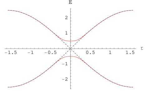
Figure 1: Time dependence of the energy levels (normalized by $D$) of the Hamiltonian (6) (solid line) at $S=4$ and $g{\mu}_{B}H/D=3.1$. Dash line shows the distance between the energy levels if they were unperturbed by the second term in Eq.  (6).

III Dynamics without noise

III.1 A single revolution

In order to describe the evolution of the magnetization in a magnetic field rotating in the $XZ$-plane, we shall compute first the probability of staying at the initial state after a rotation by 180 degrees, when a single level crossing takes place.

The Schrödinger equation for the coefficients of the wave function,

$$\left|\Psi\right\rangle=c_{-S}\left|-S\right\rangle+c_{S}\left|S\right\rangle\,,$$ (9)

can be expressed as:

$${i\hbar}\frac{d}{dt}\tilde{c}_{-S}(t)=\frac{\Delta(t)}{2}\tilde{c}_{S}(t)$$

$${i\hbar}\frac{d}{dt}\tilde{c}_{S}(t)=-h_{0}\sin(\omega t)\tilde{c}_{S}(t)+\frac{\Delta(t)}{2}\tilde{c}_{-S}(t)$$ (10)

where $\tilde{c}_{i}(t)=c_{i}(t)\exp[{\frac{i}{2\hbar}\int_{t_{0}}^{t}d{t^{\prime}}h_{0}\sin(\omega{t^{\prime}})}]$. In terms of the dimensionless variable,

$$u=\frac{h_{0}\tau}{\Delta_{0}},$$ (11)

Eq. (III.1) turns into:

$$i\frac{d}{du}\tilde{c}_{-S}(u)=\frac{{\tilde{\epsilon}}}{2}\cos^{2S}(\gamma u)\tilde{c}_{S}(u)$$

$$i\frac{d}{du}\tilde{c}_{S}(u)=-\frac{\tilde{\epsilon}}{\gamma}\sin(\gamma u)\tilde{c}_{S}(u)+\frac{{\tilde{\epsilon}}}{2}\cos^{2S}(\gamma u)\tilde{c}_{-S}(u)$$

The problem is now defined by two dimensionless parameters:

$$\tilde{\epsilon}=\frac{{\Delta_{0}}^{2}}{{\hbar\omega}\,h_{0}}\,,$$ (13)

which is similar to the parameter used in the LZS theory Garanin2 ; Dobrovitski , and

$$\gamma=\frac{\Delta_{0}}{h_{0}}\,,$$ (14)

which is a measure of the magnitude of the magnetic field. Notice that this parameter equals $\tau_{c}=\omega t_{c}$, where $t_{c}=\Delta_{0}/(\omega h_{0})$ is the characteristic time of crossing the resonance. Thus, the condition $\gamma\ll 1$ is needed for the crossing to be well localized in time on the time scale of one revolution. This condition is required for the self-consistency of the method.

From Eqs. (III.1) one can compute numerically the time evolution of the coefficients $c_{-S}$ and $c_{S}$, and, thus, the time evolution of the occupation numbers for any $\tilde{\epsilon},\gamma$. In the fast ($\tilde{\epsilon}\ll 1$) and slow ($\tilde{\epsilon}\gg 1)$ rotation regimes, analytical formulas for the occupation probabilities can be obtained. These formulas are useful for further analysis. Inspection of Eqs.(III.1) reveals that the deviation from the LZS result for slow rotation is small, since within the relevant time of the transition $\delta u\sim 1$ and $\Delta(\tau)$ is nearly constant. On the contrary, for the fast rotation regime, ($\tilde{\epsilon}\ll 1$), the relevant time interval is wider, $\delta u\sim\tilde{\epsilon}^{-1/2}$. This allows a significant change of $\Delta$ during the transition and makes possible a considerable deviation from the LZS result.

III.1.1 Fast rotation ($\tilde{\epsilon}\ll 1$)

Following the procedure devised by Garanin and Schilling Garanin2 , we can obtain the probability of staying at the initial state after a 180-degree rotation of the external magnetic field. We choose the direction of the magnetic field to be initially antiparallel to the $Z$-axis. In the zero-th order of the perturbation theory $\tilde{c_{1}}(u)=1$. In the first order, such probability is then given by

$$P=1-\frac{1}{4}\left|\frac{\tilde{\epsilon}}{\gamma}\int_{-\frac{\pi}{2}}^{\frac{\pi}{2}}\cos^{2S}(z)\exp\left[{i\frac{\tilde{\epsilon}}{\gamma^{2}}\cos(z)}\right]dz\right|^{2}$$ (15)

It is clear from this expression that for $\gamma\ll 1$, only $|z|\ll 1$ contribute to the integral. This is in accordance with the fact that the transition takes place during the time interval ${\Delta_{0}}/{h_{0}\omega}$, which is of order $\gamma$ compared with the time of the integration. Consequently, one can approximate $\cos(z)$ by

$$\cos(z)\;{\approx}\;1-\frac{z^{2}}{2}\,,\qquad\cos^{b}(z)\;{\approx}\;e^{-\frac{b}{2}z^{2}},$$ (16)

where the exponential form is chosen to insure fast convergence of the integral, and set infinite integration limits in Eq. (15):

$$P = 1-\frac{1}{4}\left|\frac{\tilde{\epsilon}}{\gamma}\int_{-\infty}^{\infty}\exp\left[{-\left(\frac{i\tilde{\epsilon}}{\gamma^{2}}+S\right)z^{2}}\right]dz\right|^{2}$$ (17)

$$= 1-\frac{\pi}{2}\frac{\tilde{\epsilon}}{\sqrt{1+{({2S\gamma^{2}}/{\tilde{\epsilon}})}^{2}}}\,.$$

\begin{picture}(12.0,5.4)\centerline{\hbox{\psfig{width=247.53888pt}}} \end{picture}

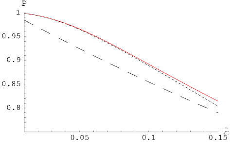
Figure 2: Probability of staying at $\left|-S\right\rangle$, $P$, as a function of parameter $\tilde{\epsilon}$ at $\gamma=0.1$ and $S=5$ . The solid line represents the numerical data, the short-dash line is the analytical result, Eq. (17), and the long-dash line is the LZS result (see explanation in the text).

The probability, $P$, of staying at the initial state $\left|-S\right\rangle$ after a 180-degree rotation is shown in Fig. 2 for different values of $\tilde{\epsilon}$. In the figure, the numerical results are compared with the result given by Eq. (17), and with the LZS result,

$$P_{LZS}=\exp[{-{\pi\tilde{\epsilon}}/{2}}]\,.$$ (18)

Note that Eq. (18) would be our result for the probability if we applied the LZS theory to the version of the Hamiltonian (6) that is linearized on $\tau$. As can be seen from Fig. 2, at $\gamma,\tilde{\epsilon}\ll 1$, Eq. (17) provides a good approximation. The difference between the numerical result and the LZS result is considerable. Fig. 3 shows $P$ for different $\gamma$ at $\tilde{\epsilon}=0.1$. Here again Eq. (17), but not the LZS formula, provides a good approximation for the $\gamma$-dependence of the staying probability.

\begin{picture}(11.0,6.0)\centerline{\hbox{\psfig{width=247.53888pt}}} \end{picture}

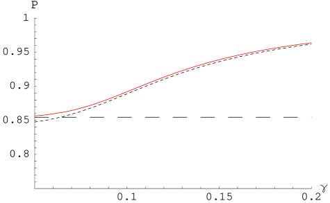
Figure 3: Probability of staying at the initial state, $P$, as a function of $\gamma$ at $\tilde{\epsilon}=0.1$ and $S=5$ . The solid line represents numerical data, the short-dash line is the analytical result Eq. (17), and the long-dash line is the LZS result.

III.1.2 Slow rotation ($\tilde{\epsilon}\gg 1$)

In the case of a slow rotation it is convenient to seek the solution of the Schrödinger’s equation in the adiabatic basis of the two-state Hamiltonian. Then, one can follow a procedure similar to that used for the fast rotation regime. The adiabatic basis is given by:

$$\left|\Psi_{\pm}\right\rangle=\frac{1}{\sqrt{2}}(\pm k_{\pm}\left|-S\right\rangle+k_{\mp}\left|S\right\rangle)$$ (19)

where

$$k_{\pm}(\tau)=\sqrt{1\pm\frac{W(\tau)}{\sqrt{W^{2}(\tau)+\Delta^{2}(\tau)}}}\,.$$ (20)

with $W(\tau)=h_{0}\sin(\tau)$ and $\Delta(\tau)=\Delta_{0}\cos^{2S}(\tau)$. The corresponding adiabatic energy levels are

$$E_{\pm}(\tau)=\pm\frac{1}{2}\sqrt{W^{2}(\tau)+\Delta^{2}(\tau)}\,.$$ (21)

Expressing the wave function as

$$\left|\Psi\right\rangle=c_{+}\left|\Psi_{+}\right\rangle+c_{-}\left|\Psi_{-}\right\rangle$$ (22)

we can now write the Schrödinger equation for

$$\tilde{c}_{\pm}(t)=\exp\left[\frac{i}{\hbar}\int{dt{E_{-}(t)}}\right]c_{\pm}(t)$$ (23)

in terms of the dimensionless variable u defined above:

$$\frac{d}{du}\,\tilde{c}_{+}=-i\tilde{\epsilon}\Omega(\gamma u)\tilde{c}_{+}-\frac{1}{2}\frac{d{w}/{du}}{(1+w^{2})}\,\tilde{c}_{-}$$

$$\frac{d}{du}\,\tilde{c}_{-}=\frac{1}{2}\frac{d{w}/{du}}{(1+w^{2})}\,\tilde{c}_{+}\,,$$ (24)

where

$$\Omega(z)=\sqrt{\frac{1}{\gamma^{2}}\sin^{2}(z)+\cos^{4S}(z)}$$ (25)

and $w(z)=W(z)/\Delta(z)$.

The asymptotic behavior of $\tilde{c}_{-}(u)$ is $\tilde{c}_{-}(u)\rightarrow 1$ for $\tilde{\epsilon}\rightarrow\infty$. At $\tilde{\epsilon}\gg 1$ the coefficient $\tilde{c}_{-}(u)$ remains close to 1. Also, far from the crossing point, $\tilde{c}_{+}(u)\approx c_{-S}$, as can be seen from Eqs. (19) and (20). These two facts allow one to obtain the probability of staying at the initial state in the first order of perturbation theory:

$$P=\frac{1}{4}\left|\int_{-\frac{\pi}{2}}^{\frac{\pi}{2}}dz\frac{d{w}/{dz}}{(1+w^{2})}\,\exp\left[{i\frac{\tilde{\epsilon}}{\gamma}\int_{0}^{z}dz^{\prime}\,\Omega(z^{\prime})}\right]\right|^{2}\,$$ (26)

At $\gamma\ll 1$ the integral is dominated by $z$ close to zero. The correct prefactor can be obtained by applying the procedure outlined in Ref. Garanin2, . With the accuracy to $\gamma^{2}$ this gives:

$$P=\exp\left\{{-\frac{\pi\tilde{\epsilon}}{2}\left[1+\left(S-\frac{1}{8}\right)\gamma^{2}\right]}\right\}$$ (27)

This probability is shown in Fig. 4 for different values of $\tilde{\epsilon}$. The numerical results are compared in the figure with the result given by Eq. (27), and with the LZS result. As can be seen from Fig. 4, at $\gamma\ll 1$, Eq. (27) provides a good approximation for $\tilde{\epsilon}>5$.

\begin{picture}(11.0,6.0)\centerline{\hbox{\psfig{width=247.53888pt}}} \end{picture}

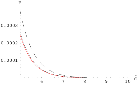
Figure 4: Probability of staying at the initial state, $P$, as a function of the parameter $\tilde{\epsilon}$ at $\gamma=0.1$ and $S=5$ . The solid line represents the numerical data, the short-dash line is the analytical result, Eq. (27), and the long-dash line is the LZS result

III.2 Continuous Rotation

Our treatment of the continuous rotation is based upon the smallness of the transition time in comparison with the period of the rotation. Periodically driven two-state systems of that kind have been studied before Kayanuma .

The individual crossing is described by the transfer matrix:

$$M=\left(\begin{array}[]{cl}\sqrt{P}&e^{-i\theta}\sqrt{1-P}\\ \\ \ -e^{i\theta}\sqrt{1-P}&\;\sqrt{P}\end{array}\right)$$ (28)

where $\theta$ is the Stokes phase given by:

$$\theta=\frac{\pi}{4}+\arg\left[\Gamma\left(1-i\frac{\tilde{\epsilon}}{4}\right)\right]+\frac{\tilde{\epsilon}}{4}\left[\ln\frac{\tilde{\epsilon}}{4}-1\right]\,.$$ (29)

This matrix transforms a given initial state into the after-crossing final state in terms of the unperturbed basis. The above expression corresponds to the crossing in which the $\left|-S\right\rangle$ level moves up towards the $\left|S\right\rangle$ level that is moving down. In the opposite case, $M$ should be replaced by the transpose matrix, $M^{T}$.

To describe the evolution of the system between crossings it must be noted that, as we have shown before, far from the crossings the unperturbed basis $\left|-S\right\rangle,\left|S\right\rangle$ almost coincides with the adiabatic basis $\left|+\right\rangle,\left|-\right\rangle$, see equations (19) and (20). In this region, the evolutions of $\left|-S\right\rangle$ and $\left|S\right\rangle$ are then considered independent, so that they can be described by the propagator

$$G_{n}=\left(\begin{array}[]{cl}\exp[(-1)^{n+1}i\alpha]&0\\ 0&\exp[(-1)^{n}i\alpha]\end{array}\right)$$ (30)

where

$$\alpha=\frac{1}{2}\left(\frac{D}{\hbar\omega}\right)\int_{0}^{\frac{\pi}{2}}d{\tau}\sqrt{W(\tau)^{2}+\Delta(\tau)^{2}}\,.$$ (31)

With the help of Eq. (28) and Eq. (30) one can compute the time evolution of the coefficients $c_{-S},c_{S}$ in Eq. (9). Starting with the initial state, the state of the system after the n-th crossing can be obtained by the successive action of $M,M^{T}$ and $G_{n}$. The time-dependence of the probability of finding a continuously rotating system in the initial state $\left|-S\right\rangle$ is shown in Fig. 5. The figure shows good agreement of the above analytical method with numerical calculation. It is important to notice that in the absence of dissipation the system does not arrive to any asymptotic state at $\tau\rightarrow\infty$. The behavior of the probability shows a long-term memory of the initial state, which is somewhat surprising. This prediction of the theory can be tested in real experiment.

\begin{picture}(11.0,5.5)\centerline{\hbox{\psfig{width=247.53888pt}}} \end{picture}

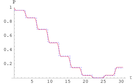
Figure 5: Time dependence of the probability of finding a continuously rotating system in the initial state $\left|-S\right\rangle$ for $\tilde{\epsilon}=0.04,\gamma=0.06$ and $S=5$. The solid line represents numerical data. The dash line shows analytical result obtained by successive application of $M,M^{T}$ and $G_{n}$.

\begin{picture}(11.0,5.5)\centerline{\hbox{\psfig{width=247.53888pt}}} \end{picture}

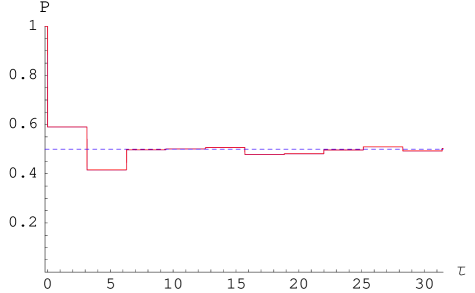
Figure 6: Time dependence of the probability of finding a particle in the state $\left|-S\right\rangle$ in the presence of a low-frequency noise for $\tilde{\epsilon}=1/3,S=10$, and $\gamma=0.01$. The plotted probability is the average over an ensemble of 20 two-state dissipative systems.

IV Dynamics with noise.

When considering the effect of the noise, it is important to distinguish between the following three regimes:

$$\gamma\ll 1\ll\omega/\Gamma$$ (32)

$$\gamma\ll\omega/\Gamma\ll 1$$ (33)

$$\omega/{\Gamma}\ll\gamma\ll 1\,$$ (34)

where $\Gamma$ is the characteristic frequency of the noise. The first of these conditions corresponds to the situation when a few revolutions may occur before any contribution of the noise becomes apparent. Consequently, during the time interval satisfying $t<1/\Gamma$ one can use the results for the probability obtained in the previous section. Under the condition (33), one can use the previously obtained results for a singular crossing but needs to take into account the destruction of the relative phase of the two states by the noise before the next crossing takes place. Under the condition (34) the results of the previous section do not apply because the coherence of the quantum state is destroyed by the noise on a timescale that is less than the crossing time.

IV.1 Low-frequency noise, $\gamma\ll\omega/\Gamma\ll 1$

The situation corresponding to the condition (33) can be easily described by the Hamiltonian

$${\cal{H}}_{eff}=-\frac{1}{2}h_{0}\sin(\tau)\sigma_{z}+\frac{1}{2}\Delta(\tau)\sigma_{x}-\eta\sigma_{z}\,,$$ (35)

where $\eta(\tau)\ll h_{0}$ is a random magnetic field in the $Z$-direction, with the correlator

$$\left\langle\eta(\tau)\eta(\tau^{\prime})\right\rangle=\eta_{0}^{2}\Theta\left[\left(\omega/\Gamma\right)-\left|\tau-\tau^{\prime}\right|\right]\,,$$ (36)

$\Theta$ being the theta-function.

The time dependence of the probability of finding the system in the state $\left|-S\right\rangle$ is shown in Fig. (6) for $\tilde{\epsilon}=1/3,S=10$, and $\gamma=0.01$. In accordance with the expectation, the probability for the system to occupy the state with $m=-S$ (or $m=S$), after going through a few oscillations, tends to the asymptotic value of 0.5. For molecular magnets, only the average of the probability over an ensemble of two-state dissipative systems is of practical importance. The probability shown in Fig. (6) is such an average.

IV.2 High-frequency noise, $\omega/{\Gamma}\ll\gamma\ll 1$

In this limit the coherence is completely suppressed, by, e.g., interaction with phonons, and the evolution of the population of energy levels must be described by the density matrix. In this case the population, $N_{-S}$, of the initially occupied state $\left|-S\right\rangle$ is given by Garanin3 ; Chudnovsky

$$\frac{d{N}_{-S}}{dt}=-\frac{\Delta(t)^{2}}{2}\frac{\hbar\Gamma}{W(t)^{2}+(\hbar\Gamma)^{2}}(N_{-S}-N_{S})\,.$$ (37)

The solution is

$$N_{-S}=\frac{1}{2}\left\{1+\exp\left[-\frac{\tilde{\epsilon}}{2}g\left(\tau;2S;{\frac{\hbar\Gamma}{h_{0}}}\right)\right]\right\}\,,$$ (38)

where $g(z;b;\alpha)$ is given by

$$g(z;b;\alpha)=$$ (39)

$$(2n+2)f_{1}(\frac{\pi}{2})-f_{1}\left(\frac{\pi}{2}-\xi\right),\;\;{\mathrm{i}f}\;\;z=(2n+1)\frac{\pi}{2}+\xi$$

$$g(z;b;\alpha)=2nf_{1}(\frac{\pi}{2})+f_{1}(\xi),\;\;{\mathrm{i}f}\;\;z=n\pi+\xi\,,$$ (40)

where $n=0,1,2...$, $\;0<\xi<\pi/2$,

$$f_{1}(z)=F_{1}\left(\frac{1}{2};\frac{1}{2}-b,1;\frac{3}{2};\sin^{2}(z),-\frac{\sin^{2}(z)}{\alpha^{2}}\right)\frac{\sin(z)}{\alpha}\;,$$ (41)

and $F_{1}(a,b_{1},b_{2};c;x,y)$ is the Appell hypergeometric function of two variables.

The time-dependence of the occupation of the state $\left|-S\right\rangle$ is shown in Fig. 7 for $\tilde{\epsilon}=1/3,S=10,\hbar\Gamma/{h_{0}}=0.01$. As in the case of a low-frequency noise, the probability to occupy either of the two levels tends to 0.5 after a few revolutions. The difference between the two regimes is that in the case of the high-frequency noise the probability monotonically approaches the asymptotic value without exhibiting any oscillation.

\begin{picture}(11.0,5.5)\centerline{\hbox{\psfig{width=247.53888pt}}} \end{picture}

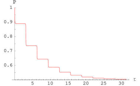
Figure 7: Time dependence of the probability of finding a particle in the state $\left|-S\right\rangle$ in the presence of a high-frequency noise for $S=10$, $\tilde{\epsilon}=1/3$ and $\frac{\Gamma}{h_{0}}=0.01$ .

V Conclusions

We have studied the equivalent of the LZS effect for a spin system in a rotating magnetic field. Typical time dependence of the probability of staying at the initial state has been computed for three different situations. The first is the situation when the noise is irrelevant on the time scale of the measurement, Fig. 5. In this case the system exhibits coherent behavior and long-term memory effects. The second situation corresponds to the noise that decohere quantum states within the time of each revolution but is slow enough to provide pure quantum dynamics during the level crossing, Fig. 6. The third situation corresponds to a very fast noise that does not allow the use of wave functions for the description of the crossing and requires the density-matrix formalism, Fig. 7. When the noise becomes important, the occupation probability of each level approaches $1/2$ after several revolutions. However, the asymptotic behavior depends on the frequency of the noise. The three regimes discussed above are given by equations (32),(33),(34). One must be able to switch between different regimes by changing the angular velocity of the rotating field and/or temperature. Experiments of that kind can shed light on the effect of dissipative environment on the resonant spin tunneling in molecular magnets. To be on a cautious side, one should notice that the evolution of the magnetization in a crystal of magnetic molecules also depends on the dipolar interactions between the molecules Prokofev ; Julio ; Gar-Sch . Our results are likely to be relevant to molecular magnets when the amplitude of the rotating field significantly exceeds dipolar fields. A candidate for such a study would be, e.g., an uniaxial Ni-4 molecular magnet that has no nuclear spins and that, with good accuracy, is described by the Hamiltonian studied in this paper.

VI Acknowledgements

This work has been supported by the NSF Grant No. EIA-0310517.

References

- (1) R. Sessoli, D. Gatteschi, A. Caneschi and M.A. Novak, Nature(London) 365, 141 (1993).
- (2) J. R. Friedman, M. P. Sarachik, J. Tejada and R. Ziolo, Phys. Rev. Lett. 76, 3830 (1996).
- (3) L.D. Landau, Phys. Z. Sowjetunion 2, 46 (1932).
- (4) C. Zener,Proc. R. Soc. London, Ser. A 137, 696 (1932).
- (5) E. C. G. Stueckelberg, Helv. Phys. Acta 5, 369 (1932).
- (6) V.V. Dobrovitski and A. D. Zvezdin, Europhys. Lett. 38, 377 (1997).
- (7) L. Gunther, Europhys. Lett. 39, 1 (1997).
- (8) V.L. Pokrovsky and N. A. Sinitsyn, Phys. Rev. B 67, 144303 (2003).
- (9) V.L. Pokrovsky and N. A. Sinitsyn, Phys. Rev. B 69, 104414 (2004).
- (10) V.L. Pokrovsky and S. Scheidl, Phys. Rev. B 70, 014416 (2004).
- (11) M. N. Leuenberger and D. Loss, Phys. Rev. B 61, 12200 (2000)
- (12) N. A. Sinitsyn and V. V. Dobrovitski, Phys. Rev. B 70, 174449 (2004).
- (13) E.M. Chudnovsky and D. A. Garanin, Phys. Rev. Lett. 87, 187203 (2001).
- (14) See, e.g., Y. Kayanuma, Phys. Rev. B 47, 9940 (1993), and references therein.
- (15) Y. Kayanuma and H. Nakayama, Phys. Rev. B 57, 13099 (1998).
- (16) D. A. Garanin, Phys. Rev. B 68, 014414 (2003).
- (17) N. A. Sinitsyn and N. Prokof‘ev, Phys. Rev. B 67, 134403(2003).
- (18) W. Wernsdorfer and R. Sessoli, Science 284, 133 (1999).
- (19) W. Wernsdorfer, S. Bhaduri, C. Boskovic, G. Christou and D. H. Hendrickson, Phys. Rev. B 65, 180403 (2002).
- (20) K. M. Mertes, Y. Suzuki, M. P. Sarachik, Y. Paltiel, H. Shtrikman, E. Zeldov, E. Rumberger, D.N. Hendrickson and G. Christou, Phys. Rev. Lett. 87, 227205 (2001).
- (21) E. del Barco, A. D. Kent, E. M. Rumberger, D. N. Hendrikson and G. Christou, Europhys. Lett. 60, 768 (2002); E. del Barco, A. D. Kent, S. Hill, J. M. North, N. S. Dalal, E. M. Rumberger, D. N. Hendrikson, N. Chakov and G. Christou, arXiv:cond-mat/0404390 (2004).
- (22) J. L. van Hemmen and A. Suto, J. Phys.: Condens. Matter 9 3089 (1997).
- (23) D.A. Garanin, J. Phys. A 24, L61 (1991).
- (24) D. A. Garanin and R. Schilling, Phys. Rev. B 66, 174438 (2002).
- (25) D.A. Garanin and E.M. Chudnovsky, Phys. Rev. B 56, 11102 (1997).
- (26) N. V. Prokof’ev and P. C. E. Stamp, Phys. Rev. Lett. 80, 5794 (1998).
- (27) J. F. Fernandez and J. J. Alonso, Phys. Rev. Lett. 91, 047202 (2003).
- (28) D. A. Garanin and R. Schilling, ArXiv:cond-mat/0501089 (2005).