Berry phase of magnons in textured ferromagnets

Abstract

We study the energy spectrum of magnons in a ferromagnet with topologically nontrivial magnetization profile. In the case of inhomogeneous magnetization corresponding to a metastable state of ferromagnet, the spin-wave equation of motion acquires a gauge potential leading to a Berry phase for the magnons propagating along a closed contour. The effect of magnetic anisotropy is crucial for the Berry phase: we show that the anisotropy suppresses its magnitude, which makes the Berry phase observable in some cases, similar to the Aharonov-Bohm effect for electrons. For example, it can be observed in the interference of spin waves propagating in mesoscopic rings. We discuss the effect of domain walls on the interference in ferromagnetic rings, and propose some experiments with a certain geometry of magnetization. We also show that the nonvanishing average topological field acts on the magnons like a uniform magnetic field on electrons. It leads to the quantization of the magnon spectrum in the topological field.

I Introduction

The Berry phase theory berry84 ; shapere89 ; bohm03 allowed to generalize the idea of Aharonov-Bohm effect aharonov59 on electrons in the electromagnetic potential, to an analogous effect related to a gauge potential, which arises during the adiabatic motion of a quantum system in a parametric space. Up to now a lot of efforts has been directed to understand better and to find an experimental confirmation for the Berry phase of electrons like, for example, in the case of electrons moving in a varying magnetization field of the inhomogeneous ferromagnet. lyanda98 ; ye99

One of the most intriguing consequences of the Berry phase theory is a possibility of the Aharonov-Bohm-like effect on electrically neutral particles or boson fields.anandan82 ; chiao86 An example of the adiabatic phase for the polarized light has been investigated by Pancharatnam pancharatnam56 and Berry. berry87 The other example is the Aharonov-Bohm effect for the exciton,romer00 which is a bound state of an electron and a hole in semiconductors.

Here we consider the effect of the gauge potential and Berry phase on the propagation of magnons in textured ferromagnets. Such quasiparticles are usually viewed as the elementary excitations of the ordered homogeneous state of a ferromagnet but they can be also used to classify the excited states near a metastable inhomogeneous magnetic configuration. These magnons describe the dynamics of weakly excited inhomogeneous ferromagnet.

The dynamics of magnetization in nanomagnets is in the focus of recent activitydynamics because of the importance of this problem for magnetoelectronic applications.wolf01 ; zutic04 It includes the switching of magnetization by electric current, spin pumping, magnetization reversal in microscopic spin valves, etc. Usually, the magnons play a negative role in the magnetization dynamics limiting the frequency of magnetic reversal, and also leading to the energy dissipation. However, they can be probably used in the spin transport phenomena like the spin currents of magnetically polarized electrons.

Here we study the energy spectrum of spin waves in ferromagnets with a static inhomogeneous magnetization profile, and we demonstrate a possibility of observation of the Berry phase in the interference experiments on spin waves in magnetic nanostructures. Recent results of the micromagnetic computer simulationyamasaki03 ; ha03 ; hertel03 of such systems demonstrate that the interference of spin waves can be really observed in magnetic nanorings with domain walls.

The equation for spin wave excitations in a general case of arbitrary local frame depending on both coordinate and time, has been found long ago by Korenman et alkorenman77 in the context of local-band theory of itinerant magnetism.korenman Here we use an idea of this method to relate the adiabatic space transformation to the Berry phase and to find corresponding properties of the spin waves in a topologically nontrivial inhomogeneous magnetic profile, which is a metastable state of the ferromagnet. We show that the magnetic anisotropy is a crucial element determining the possibility of observation of the Berry phase in real experiments.

II Model and spin wave equations

We consider the model of a ferromagnet described by the Hamiltonian, which includes the exchange interaction, anisotropy, and the interaction with external magnetic field . It has the following general form

$$H=\frac{1}{2}\int d^{3}{\bf r}\left[a\left(\frac{\partial n_{\mu}({\bf r})}{\partial r_{i}}\right)^{2}+\mathcal{F}\left\{{\bf n}({\bf r})\right\}\right],$$ (1)

where ${\bf n}({\bf r})$ is the unit vector oriented along the magnetization ${\bf M}({\bf r})$ at the point ${\bf r}$, $a$ is the constant of exchange interaction, $\mathcal{F}\left\{{\bf n}({\bf r})\right\}$ is a function determining the magnetic anisotropy [correspondingly, it includes a certain number of tensors relating the components of vector ${\bf n}({\bf r})$] and the dependence on external field, and $M_{0}$ is the magnitude of magnetization.

Due to the condition ${\bf n}^{2}({\bf r})=1$, the model is constrained and belongs to the class of nonlinear $\sigma$ models.nagaosa99 The stationary (saddle point) solutions for the magnetization vector ${\bf n}_{0}({\bf r})$ describing metastable states of the ferromagnet, can be found by minimizing Hamiltonian (1) with the constraint ${\bf n}^{2}({\bf r})=1$. It was shown (see, e.g., Refs. [belavin75, ; pokrovsky88, ]) that such metastable states with inhomogeneous magnetization profile are related to the topology of ferromagnetic ordering, and they can include skyrmions, magnetic vortices, and other topological objects.

We will be interested in describing the dynamics of small deviations $\delta{\bf n}({\bf r})$ from a certain metastable profile ${\bf n}_{0}({\bf r})$ with a nonuniform magnetization, ${\bf n}({\bf r})={\bf n}_{0}({\bf r})+\delta{\bf n}({\bf r})$, $\left|\delta{\bf n}({\bf r})\right|\ll 1$. Correspondingly, we assume that the solution of a saddle-point equation describing the state ${\bf n}_{0}({\bf r})$ is already known.

We perform a local transformation

$$\tilde{\bf n}({\bf r})={\rm R}({\bf r})\,{\bf n}({\bf r}),$$ (2)

using the orthogonal transformation matrix ${\rm R}({\bf r})$. By definition, it determines the rotation of local frame in each point of the space, so that the magnetization in the local frame is oriented along the $z$ axis, $\tilde{\bf n}_{0}=(0,\,0,\,1)$. Then we consider small deviations of magnetization ${\bf s}({\bf r})$ from $\tilde{\bf n}_{0}$. Since ${\bf s}({\bf r})$ is small and vectors $\tilde{\bf n}_{0}$ are oriented along $z$, the vectors ${\bf s}({\bf r})$ lie in the $x$-$y$ plane.

The transformation matrix in Eq. (2) is taken in a general form of orthogonal transformation

$${\rm R}({\bf r})=e^{i\psi({\bf r})\,J_{z}}\,e^{i\theta({\bf r})\,J_{y}}\,e^{i\phi({\bf r})\,J_{z}}\,,$$ (3)

where $\psi$, $\theta$, $\phi$ are the Euler angles determining an arbitrary rotation of the coordinate frame, and $J_{x}$, $J_{y}$, and $J_{z}$ are the generators of 3D rotations around $x$, $y$ and $z$ axes.

Two rotation parameters (for definiteness, the angles $\theta$ and $\phi$) can be used to define the frame with the $z$ axis along the vector ${\bf n}_{0}({\bf r})$. In the absence of anisotropy, the additional rotation to the angle $\psi$ is purely gauge transformation. However, in a general case of anisotropic system, this rotation allows to choose the local frame in correspondence with the orientation of anisotropy axes.

The Hamiltonian of exchange interaction (the first term in Eq. (1)) in the rotated frame has the following form

$$H_{ex}=\frac{a}{2}\int d^{3}{\bf r}\left(\frac{\partial\tilde{n}_{\mu}}{\partial r_{i}}-A_{i}^{\mu\nu}\tilde{n}_{\nu}\right)^{2},$$ (4)

where the gauge field $A_{i}({\bf r})$ is defined by

$$A_{i}({\bf r})=\left(\frac{\partial}{\partial r_{i}}\;{\rm R}\right)\,{\rm R}^{-1}.$$ (5)

Transformation (3) and gauge potential (5) are $3\times 3$ matrices acting on the magnetization vectors. The matrix $A_{i}({\bf r})$ can be also presented as

$$A_{i}({\bf r})=i\mathcal{A}^{\mu}_{i}({\bf r})\,J_{\mu},$$ (6)

where $\mathcal{A}^{\mu}_{i}({\bf r})$ belongs to the adjoint representation of the rotation group.

Using (3) and (6), we find the explicit dependence of the gauge potential on the Euler angles

$$\mathcal{A}^{x}_{i}({\bf r})=\sin\psi\;\frac{\partial\theta}{\partial r_{i}}-\sin\theta\;\cos\psi\;\frac{\partial\phi}{\partial r_{i}}\;,$$

$$\mathcal{A}^{y}_{i}({\bf r})=\cos\psi\;\frac{\partial\theta}{\partial r_{i}}+\sin\theta\sin\psi\;\frac{\partial\phi}{\partial r_{i}}\;,$$ (7)

$$\mathcal{A}^{z}_{i}({\bf r})=\frac{\partial\psi}{\partial r_{i}}+\cos\theta\;\frac{\partial\phi}{\partial r_{i}}\;.\hskip 28.45274pt$$

The magnetic anisotropy described by the second term in the right hand part of (1) gives after transformation to the local frame a function $\tilde{\mathcal{F}}\left\{\tilde{\bf n}({\bf r})\right\}$ with correspondingly transformed tensor fields. Here we do not restrict the general consideration of the problem by any specific form of the anisotropy but in the following we consider the most important examples of easy plane and easy axis anisotropy.

The Landau-Lifshitz equations for the magnetization in the locally transformed frame are

$$\frac{\partial\tilde{n}_{\mu}}{\partial t}=-\frac{\gamma}{M_{0}}\;\epsilon_{\mu\nu\lambda}\,\tilde{n}_{\nu}\left(\frac{\delta H}{\delta\tilde{n}_{\lambda}}-\nabla^{\lambda\rho}_{i}\,\frac{\delta H}{\delta\,(\nabla^{\rho\tau}_{i}\,\tilde{n}_{\tau})}\right),$$ (8)

where $\epsilon_{\mu\nu\lambda}$ is the unit antisymmetric tensor, and

$$\nabla^{\mu\nu}_{i}=\frac{\partial}{\partial r_{i}}\;\delta_{\mu\nu}-A_{i}^{\mu\nu}$$ (9)

is the covariant derivative. The right-hand part of Eq. (8) vanishes for the magnetization profile corresponding to a metastable state. This is seen from the Landau-Lifshitz equation in the unrotated original frame. In the following, we will use Eq. (8) for the small deviations of magnetization from the metastable state. Hence, we will consider in the right part of (8) only the terms linear in deviations.

Using (1), (4) and (8) we find the equations for weak magnetic excitations near the metastable state (spin waves)

$$\frac{\partial s_{x}}{\partial t}=-c_{s}\left[\frac{\partial^{2}s_{y}}{\partial r_{i}^{2}}-2\mathcal{A}^{z}_{i}\,\frac{\partial s_{x}}{\partial r_{i}}-(\mathcal{A}^{z}_{i})^{2}\,s_{y}\right.$$

$$\left.-\frac{\partial\mathcal{A}^{z}_{i}}{\partial r_{i}}\;s_{x}+\,(\mathcal{A}^{y}_{i})^{2}\,s_{y}+\mathcal{A}^{x}_{i}\,\mathcal{A}^{y}_{i}\,s_{x}\right]$$

$$+\frac{\gamma}{M_{0}}\;\frac{\partial^{2}\tilde{\mathcal{F}}}{\partial\tilde{n}_{x}\,\partial\tilde{n}_{y}}\;s_{x}+\,\frac{\gamma}{M_{0}}\;\frac{\partial^{2}\tilde{\mathcal{F}}}{\partial\tilde{n}_{y}^{2}}\;s_{y}\;,$$ (10)

$$\frac{\partial s_{y}}{\partial t}=c_{s}\left[\frac{\partial^{2}s_{x}}{\partial r_{i}^{2}}+2\mathcal{A}^{z}_{i}\,\frac{\partial s_{y}}{\partial r_{i}}-(\mathcal{A}^{z}_{i})^{2}s_{x}\right.$$

$$\left.+\frac{\partial\mathcal{A}^{z}_{i}}{\partial r_{i}}\;s_{y}+\,(\mathcal{A}^{x}_{i})^{2}\,s_{x}+\mathcal{A}^{x}_{i}\,\mathcal{A}^{y}_{i}\,s_{y}\right]$$

$$-\frac{\gamma}{M_{0}}\;\frac{\partial^{2}\tilde{\mathcal{F}}}{\partial\tilde{n}_{x}\,\partial\tilde{n}_{y}}\;s_{y}-\,\frac{\gamma}{M_{0}}\;\frac{\partial^{2}\tilde{\mathcal{F}}}{\partial\tilde{n}_{x}^{2}}\;s_{x}\;,$$ (11)

where $c_{s}=\gamma a/M_{0}$ is the stiffness.

Using (10) and (11) we can also present the equations for circular components of the spin wave, $s_{\pm}=s_{x}\pm is_{y}$,

$$\pm\,i\;\frac{\partial s_{\pm}}{\partial t}=\left[-c_{s}\left(\frac{\partial}{\partial r_{i}}\mp iA^{z}_{i}\right)^{2}-V({\bf r})+\frac{\gamma}{2M_{0}}\;\frac{\partial^{2}\tilde{\mathcal{F}}}{\partial\tilde{n}_{x}^{2}}\right.$$

$$\left.+\frac{\gamma}{2M_{0}}\;\frac{\partial^{2}\tilde{\mathcal{F}}}{\partial\tilde{n}_{y}^{2}}\right]s_{\pm}+\left[-w({\bf r})-ic_{s}\,\mathcal{A}^{x}_{i}\mathcal{A}^{y}_{i}\right.$$

$$\left.+\,\frac{i\gamma}{M_{0}}\;\frac{\partial^{2}\tilde{\mathcal{F}}}{\partial\tilde{n}_{x}\,\partial\tilde{n}_{y}}+\frac{\gamma}{2M_{0}}\;\frac{\partial^{2}\tilde{\mathcal{F}}}{\partial\tilde{n}_{x}^{2}}-\frac{\gamma}{2M_{0}}\;\frac{\partial^{2}\tilde{\mathcal{F}}}{\partial\tilde{n}_{y}^{2}}\right]s_{\mp}\,,\hskip 8.5359pt$$ (12)

where $V({\bf r})$ and $w({\bf r})$ are, respectively, the effective potential and a mixing field acting on the spin wave:

$$V({\bf r})=\frac{c_{s}}{2}\,\left[\left(\mathcal{A}^{x}_{i}\right)^{2}+\left(\mathcal{A}^{y}_{i}\right)^{2}\right],$$ (13)

$$w({\bf r})=\frac{c_{s}}{2}\,\left[\left(\mathcal{A}^{x}_{i}\right)^{2}-\left(\mathcal{A}^{y}_{i}\right)^{2}\right].$$ (14)

Equations (12) for $s_{+}({\bf r},t)$ and $s_{-}({\bf r},t)$ are complex conjugate to each other since they both describe the same spin wave with real components $s_{x}({\bf r},t)$ and $s_{y}({\bf r},t)$.

We can see that $V({\bf r})$ is an effective potential profile for the propagation of spin wave. Due to the terms $w({\bf r})$ and $ic_{s}\mathcal{A}_{i}^{x}\mathcal{A}_{i}^{y}$ in (12), the equations for circular components $s_{+}$ and $s_{-}$ are coupled even in the absence of anisotropy. All these terms are of the second order in derivative of the rotation angle, and they are small in the adiabatic limit corresponding to a smooth variation of the magnetization vector ${\bf n}({\bf r})$.

III Semiclassical approximation

Equations (10) and (11) can be solved in the semiclassical approximation. The condition of its applicability is a smooth variation of gauge potential $\mathcal{A}^{\mu}_{i}({\bf r})$ and fields related to the anisotropy, as well as the external magnetic field, at the wavelength of the spin wave, $kL\gg 1$, where $k$ is the wavevector of the spin wave and $L$ is the characteristic length of the variation of $\mathcal{A}^{\mu}_{i}({\bf r})$ and $\mathcal{F}\left\{{\bf n}({\bf r})\right\}$ (more exactly, the minimum of the corresponding characteristic lengths). Note that the condition of applicability of the semiclassical approximation to solve the spin-wave equations, does not require any smallness of the gauge potential itself.

Starting from Eqs. (10) and (11), we look for a general semiclassical solution in the form

$$s_{x}({\bf r},t)=a\,\cos\left[\xi({\bf r})-\omega t\right]+b\,\sin\left[\xi({\bf r})-\omega t\right],$$ (15)

$$s_{y}({\bf r},t)=d\,\sin\left[\xi({\bf r})-\omega t\right]+f\,\cos\left[\xi({\bf r})-\omega t\right],$$ (16)

with arbitrary coefficients $a$, $b$, $d$, $f$, and a smooth function $\xi({\bf r})$, so that we can neglect the second derivative of $\xi({\bf r})$ over coordinate ${\bf r}$. Substituting (15) and (16) in (10) and (11), we can find four equation for the $a$, $b$, $d$, $f$ coefficients.

The solution (15), (16) describes the elliptic spin wave with an arbitrary choice of the axes $x$ and $y$, and, generally, with a varying in space orientation of the principal axes of the ellipse. We can simplify our consideration by choosing the angle $\psi({\bf r})$ at each point of the space in accordance with the orientation of the principal axes. The corresponding equation for $\psi({\bf r})$ can be found from the condition of $b=f=0$ in Eqs. (15) and (16)

$$c_{s}\,\mathcal{A}^{x}_{i}\,\mathcal{A}^{y}_{i}-\frac{\gamma}{M_{0}}\;\frac{\partial^{2}\tilde{\mathcal{F}}}{\partial\tilde{n}_{x}\,\partial\tilde{n}_{y}}=0.$$ (17)

Using (17) and neglecting the terms with derivative of $\mathcal{A}_{i}^{z}$, which are small in the semiclassical approximation, we write the spin-wave equations (10) and (11) as

$$\frac{\partial s_{x}}{\partial t}=-c_{s}\left[\frac{\partial^{2}s_{y}}{\partial r_{i}^{2}}-2\mathcal{A}^{z}_{i}\,\frac{\partial s_{x}}{\partial r_{i}}-(A^{z}_{i})^{2}\,s_{y}+\,(\mathcal{A}^{y}_{i})^{2}\,s_{y}\right]$$

$$+\,\frac{\gamma}{M_{0}}\;\frac{\partial^{2}\tilde{\mathcal{F}}}{\partial\tilde{n}_{y}^{2}}\;s_{y}\;,\hskip 14.22636pt$$ (18)

$$\frac{\partial s_{y}}{\partial t}=c_{s}\left[\frac{\partial^{2}s_{x}}{\partial r_{i}^{2}}+2\mathcal{A}^{z}_{i}\,\frac{\partial s_{y}}{\partial r_{i}}-(\mathcal{A}^{z}_{i})^{2}s_{x}+\,(\mathcal{A}^{x}_{i})^{2}\,s_{x}\right]$$

$$-\,\frac{\gamma}{M_{0}}\;\frac{\partial^{2}\tilde{\mathcal{F}}}{\partial\tilde{n}_{x}^{2}}\;s_{x}\;.\hskip 14.22636pt$$ (19)

Note that by fixing the angle $\psi$ in Eq. (17), we are choosing the gauge, which defines completely the potential $\mathcal{A}_{i}^{\mu}$. We do it in spirit of the usual fixing gauge in the WKB approximation.

After substitution of (15) and (16) with $b=f=0$ into (18) and (19), we come to the following equation for the momentum $k_{i}({\bf r})\equiv\partial\xi({\bf r})/\partial r_{i}$

$$\left(\omega+2c_{s}\,\mathcal{A}^{z}_{i}\,k_{i}\right)^{2}-\left\{c_{s}\left[k_{i}^{2}+(\mathcal{A}^{z}_{i})^{2}-(\mathcal{A}^{y}_{i})^{2}\right]\right.$$

$$\left.+2p_{x}\right\}\left\{c_{s}\left[k_{i}^{2}+(\mathcal{A}^{z}_{i})^{2}-(\mathcal{A}^{x}_{i})^{2}\right]+2p_{y}\right\}=0,\hskip 2.84544pt$$ (20)

where

$$p_{x,y}({\bf r})=\frac{\gamma}{2M_{0}}\;\frac{\partial^{2}\tilde{\mathcal{F}}}{\partial\tilde{n}_{x,y}^{2}}\;$$ (21)

are the anisotropy parameters.

Equation (20) should be solved for $k_{i}({\bf r})$ as a function of smooth inhomogeneous field $\mathcal{A}_{i}^{\mu}({\bf r})$. This equation does not constraint the orientation of ${\bf k}({\bf r})$ but determines the magnitude of vector ${\bf k}({\bf r})$ for each direction in the momentum space. Let us take vector ${\bf k}({\bf r})$ along an arbitrary direction, defined by a unity vector ${\bf g}$. Then we can rewrite (20) as

$$\left[\omega+2c_{s}k\,g_{i}\mathcal{A}^{z}_{i}\right]^{2}-\left\{c_{s}\left[k_{i}^{2}+(\mathcal{A}^{z}_{i})^{2}-(\mathcal{A}^{x}_{i})^{2}\right]+2p_{x}\right\}$$

$$\times\left\{c_{s}\left[k_{i}^{2}+(\mathcal{A}^{z}_{i})^{2}-(\mathcal{A}^{y}_{i})^{2}\right]+2p_{y}\right\}=0,\hskip 14.22636pt$$ (22)

and we come to the fourth-order algebraic equation for $k({\bf r})$. It can be solved numerically, and a resulting dependence of $k_{i}({\bf r})$ on the gauge field in the integral $\xi({\bf r})=\int_{C}k_{i}({\bf r})\,dr_{i}$ leads to the Berry phase acquired by the spin wave propagating along the contour $C$.

We can find the solution of Eq. (22) analytically in the limit of weak gauge potential $\left|\mathcal{A}^{z}_{i}\right|\ll k$, which corresponds to the adiabatic variation of the magnetization direction ${\bf n}({\bf r})$ and also the adiabatic rotation in space of the elliptic trajectory, $\left|\partial\psi/\partial r_{i}\right|\ll k$. Then in the first order of $\mathcal{A}_{i}^{z}$ we find

$$k_{i}({\bf r})\simeq\frac{g_{i}}{\sqrt{c_{s}}}\left[\left(\omega^{2}+p^{2}\right)^{1/2}-p\,\right]^{1/2}$$

$$+\,g_{i}\,g_{j}\,\mathcal{A}^{z}_{j}({\bf r})\,\left(1+p^{2}/\omega^{2}\right)^{-1/2},$$ (23)

where $p=\left|p_{x}-p_{y}\right|$.

Using Eq. (23) and taking the vector ${\bf g}$ along the tangent at each point of a closed contour $C$, we find the Berry phase

$$\gamma_{B}(C)=\oint_{C}\;\frac{\mathcal{A}^{z}_{i}({\bf r})\,dr_{i}}{\left(1+p^{2}/\omega^{2}\right)^{1/2}}\;.$$ (24)

As follows from (24), the Berry phase $\gamma_{B}(C)$ in the anisotropic system acquires an additional factor $\kappa\equiv\left(1+p^{2}/\omega^{2}\right)^{-1/2}$ depending on the magnetic anisotropy parameter $p$.

The denominator in (24) has a simple geometrical interpretation. Indeed, the coefficients $a$ and $d$ in the semiclassical solution (15), (16) are the ellipse parameters, which are related to the anisotropy factor $p$

$$\frac{a}{d}=\left(1+\frac{p^{2}}{\omega^{2}}\right)^{1/2}-\frac{p}{\omega}\;.$$ (25)

Correspondingly, we can relate the parameter $\kappa=\left(1+p^{2}/\omega^{2}\right)^{-1/2}$ in Eq. (24) to the geometry parameters of the ellipse

$$\kappa=\sin 2\Theta,$$ (26)

where $\Theta=\arctan(d/a)$.

Using definition (7), the Berry phase can be finally presented as

$$\gamma_{B}(C)=\oint_{C}\;\left[\left(\kappa-1\right)\frac{\partial(\psi+\phi)}{\partial r_{i}}+\kappa\left(\cos\theta-1\right)\;\frac{\partial\phi}{\partial r_{i}}\right]dr_{i}.$$ (27)

In this expression we extracted a term proportional to $2\pi N$, $N\in\mathbf{Z}$. This allows to avoid the multivaluedness of Berry phase in the absence of anisotropy when $\kappa=1$.bruno04 The first term in (27) is proportional to the total winding number of rotations associated with the angles $\psi$ and $\phi$, whereas the second term is a spherical angle on $S_{2}$, which is the mapping space of the vector field ${\bf n}({\bf r})$. The second term in (27) has a standard interpretation of the Berry phase as the magnetic flux penetrating the contour on $S_{2}$, when the field is created by monopole at the center of Berry sphere. Following this idea, one can interpret the first term in (27) as the flux created by the magnetic string along the $z$ axis, penetrating through the mapping contour on the unit circle.bruno04 In accordance with Eq. (27), this contribution to the Berry phase vanishes for isotropic magnetic systems, $\kappa=1$. The first term in (27) is the topological Berry phase (it depends only on the winding number) in contrast to the geometric Berry phase of the second term in (27).bruno04

As follows from (24), the effective gauge field for spin waves in the anisotropic system is $\tilde{\mathcal{A}}_{i}=\kappa\mathcal{A}^{z}_{i}$, and the corresponding topological field acting on the magnons can be calculated as the curvature of connection $\tilde{\mathcal{A}}_{i}({\bf r})$

$$B_{i}=\kappa\;\epsilon_{ijk}\;\frac{\partial\mathcal{A}_{k}^{z}}{\partial r_{j}}+\epsilon_{ijk}\;\frac{\partial\kappa}{\partial r_{j}}\;\mathcal{A}_{k}^{z}\,.$$ (28)

Note that there is a contribution related to the variation in space of the anisotropy parameters [second term in Eq. (28)].

We consider now in more details the motion of elliptic spin wave in the adiabatic regime. The anisotropy suppresses one of the components $s_{x}$ or $s_{y}$ breaking the symmetry with respect to rotations around $z$ axis. Correspondingly, there is no gauge invariance $s_{+}\rightarrow e^{i\varphi}s_{+}$ and $s_{-}\rightarrow e^{-i\varphi}s_{-}$ for the circular components, and the motion of magnetization in the spin wave is elliptical. In the adiabatic limit of $\left|\mathcal{A}^{z}_{i}\right|\ll k$, the solutions for $s_{x}$ and $s_{y}$ are given by Eqs.  (15) and (16) with $b=f=0$ and the ratio of amplitudes $(a/d)$. Thus, we could expect the local invariance to transformations preserving the value of $s_{x}^{2}+(d/a)^{2}s_{y}^{2}=const$ instead of simple rotations in $x-y$ plane.

Using the Fourier transformation of Eqs. (18) and (19) for $s_{x,y}$ we find the following equation for the elliptic components of spin wave, $\tilde{s}_{\pm}=s_{x}\pm i(d/a)\,s_{y}$

$$\left[\omega+2c_{s}k_{i}\mathcal{A}^{z}_{i}-\tilde{c}_{s}\left\{k_{i}^{2}+(\mathcal{A}^{z}_{i})^{2}\right\}-\frac{pd}{2a}\right]\tilde{s}_{+}$$

$$-\frac{a}{2d}\left[c_{s}\left\{(k_{i}^{2}+(\mathcal{A}^{z}_{i})^{2}\right\}\left(1-\frac{d^{2}}{a^{2}}\right)-\frac{pd^{2}}{a^{2}}\right]\tilde{s}_{-}=0,\hskip 8.5359pt$$ (29)

and the complex conjugate to (29), where $\tilde{c}_{s}=c_{s}\,(1+d^{2}/a^{2})a/2d\,$, and we determine the $d/a$ from the condition of vanishing of the second bracket in Eq. (29). This condition determines the ellipticity factor, and we find that it coincides with Eq. (25) in the limit of $\left|\mathcal{A}^{z}_{i}\right|\ll k$. Thus, we come to the following equation for the elliptic wave in the gauge field

$$\left\{\omega+2c_{s}k_{i}\mathcal{A}^{z}_{i}-\tilde{c}_{s}\left[k_{i}^{2}+(\mathcal{A}^{z}_{i})^{2}\right]-\frac{pd}{2a}\right\}\tilde{s}_{+}=0.\hskip 8.5359pt$$ (30)

This equation is not gauge invariant but in the adiabatic regime, neglecting the difference in small terms of the order of $(\mathcal{A}^{z}_{i})^{2}$, we can present it as

$$\left[\omega-\tilde{c}_{s}\left(k_{i}-\kappa\,\mathcal{A}^{z}_{i}\right)^{2}-\frac{pd}{2a}\,\right]\tilde{s}_{+}=0.$$ (31)

Equation (31) contains a factor $\kappa<1$ before $\mathcal{A}^{z}_{i}$ and formally looks like the equation of motion of a particle moving in the reduced gauge field, which in turn leads to an effective suppression of the Berry phase. The calculation of Berry phase using Eq. (31) with the gauge field suppressed by factor $\kappa$ leads us again to Eq. (24).

In the absence of anisotropy and in the adiabatic approximation, the solution of spin wave equations has a simple form. The equations for circular components (12) are separated

$$\pm\,i\;\frac{\partial s^{(0)}_{\pm}}{\partial t}=-c_{s}\left(\frac{\partial}{\partial r_{i}}\mp i\mathcal{A}^{z}_{i}\right)^{2}s^{(0)}_{\pm}\,,$$ (32)

and the corresponding solution is

$$s_{+}({\bf r},t)\sim\exp\left[i\int k_{i}({\bf r})\,dr_{i}-i\omega t\right],$$ (33)

with $k_{i}({\bf r})\simeq g_{i}\omega/c_{s}^{1/2}+g_{i}g_{j}\,\mathcal{A}_{j}^{z}({\bf r})$. The spin wave propagating along a closed contour $C$ acquires the Berry phase of Eq. (24) with $p=0$.

Using Eqs. (7) we can present the topological field (28) in the absence of anisotropy as

$$B_{i}=-\sin\theta\;\epsilon_{ijk}\;\frac{\partial\theta}{\partial r_{j}}\,\frac{\partial\phi}{\partial r_{k}}.$$

It does not depend on the angle $\psi$, related to the choice of gauge like in the case of electromagnetism.

By creating a certain metastable configuration of the magnetization ${\bf n}_{0}({\bf r})$ in the ferromagnet, we simulate an effective gauge potential $\tilde{\mathcal{A}}_{i}({\bf r})$, acting on the spin waves similar to the magnetic field in case of electrons. In particular, when the averaged in space topological field (28) is not zero, there arises the Landau quantization of the energy spectrum of magnons. In the absence of anisotropy, we find the quantized spectrum $\hbar\omega_{n}=2\hbar c_{s}\left|\left<{\bf B}\right>\right|(n+1/2)$, where $\left<...\right>$ means the average in space.

IV Interference of spin waves in mesoscopic rings

Let us consider now the ring geometry of a ferromagnet with a topologically nontrivial metastable magnetization ${\bf n}_{0}({\bf r})$. It can be, for example, a magnetization vortex (Fig. 1a) or an even number of domain walls in one branch of the ring like presented in Fig. 1b. Such a magnetization profile presents a metastable magnetic state.

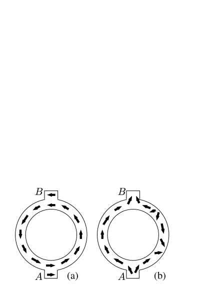
Figure 1: Two rings with topologically nontrivial magnetization field.

Let us consider first the case when there is no anisotropy. If $kL\ll 1$ (adiabatic regime), the low-energy magnetic excitations of the metastable state are described by Eq. (32). Due to the presence of gauge potential $\mathcal{A}^{z}_{i}({\bf r})$, there is a phase shift of waves propagating from the point $A$, where the waves are excited, to the observation point $B$ (see Fig. 1). The phase shift (Berry phase) equals to the integral $\oint\mathcal{A}^{z}_{i}({\bf r})\,dr_{i}$ along the ring, and by using Stokes theorem can be calculated as the flux $\Phi$ of topological field $B$ defined in Eq. (34). It can be also presented as the spherical angle enclosed by the mapping of the ring to the circle at the unit sphere $S_{2}$. This way we can find the phase shift of $2\pi$ and $\pi N_{d}$ for Figs. 1a and 1b, respectively, where an even $N_{d}$ is the number of domain walls in the right arm of the ring. For example, in the case of Fig. 1b with two domain walls in the right arm, there is no interference of spin waves excited in $A$ and coming to the point $B$ because the corresponding phase shift is $2\pi$.

In the absence of anisotropy, the interference in the ring can be induced by rotating all magnetic moments from the plane to a certain angle $\alpha$ (the corresponding mapping is presented in Fig. 2b). The Berry phase associated with the path along the ring will be smaller than $2\pi$. For $\alpha=\pi/6$ the Berry phase turns out to be $\pi$. It means that the experiment with interference of spin waves propagating from $A$ to $B$ through two different arms of the ring, would result in a complete suppression of the outgoing from $B$ spin wave. Physically, it can be realized using the ring with very small easy-plane anisotropy, $p/\omega\ll 1$ in a weak external magnetic field along $z$ axis.

A similar idea was recently proposed by Schütz et al schutz03 for the radial orientation of magnetic moments under inhomogeneous magnetic field directed from some point at the axis of the ring. This magnetic field creates a ”crown” of magnetic moments, and the corresponding mapping is similar to that presented in Fig. 2b.

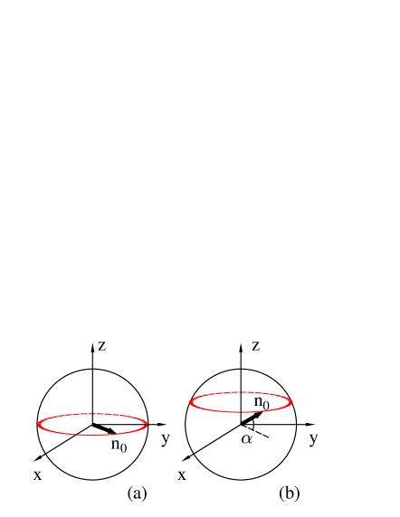
Figure 2: Mapping of the ring to the ${\bf n}$-space $S_{2}$ (red contour) in the case of in-plane vortex magnetization shown in Fig.1a (a) and for the same geometry with magnetization vector deviating from the plane to the angle $\alpha$ (b). The Berry phase is $2\pi$ in case (a) and $\pi$ for $\alpha=\pi/6$ in case (b).

However, in the case of nonvanishing easy-plane anisotropy, there is no need to apply magnetic field to provide the interference of spin waves propagating in the geometry of Fig. 1b. In this case the Berry phase is given by Eq. (27) with $p=\gamma\lambda/2M_{0}=const$, and we obtain the difference in phases for two waves $\Delta\gamma_{B}=\pi N_{d}/(1+p^{2}/\omega^{2})^{1/2}$. Thus, the interference of spin waves should be clearly seen for the two-arm geometry with domain walls. The computer simulation experiments hertel03 confirm this expectation.

Figure 3: Spin waves on a wide ring (thin-wall cylinder made of easy-plane ferromagnetic ribbon). The magnetization is along axis $z$.

Another possibility to observe the interference of spin waves can be presented by the geometry of a wide ring (thin-wall cylinder) like presented in Fig. 3. Assuming the easy-plane anisotropy of the ribbon, we obtain the ground state with a homogeneous magnetization along the axis of cylinder. The anisotropy axis is oriented radially in each point of the cylinder, and the corresponding local frame is shown in the figure as $x^{\prime}\,y^{\prime}\,z^{\prime}$. Due to the homogeneous magnetization, we get $\theta=0$, and from (7) we obtain $\mathcal{A}^{z}_{i}({\bf r})=\partial(\psi+\phi)/\partial r_{i}$. The components of anisotropy vector are $u_{x}=\cos\varphi$ and $u_{y}=\sin\varphi$. Using Eq. (34) we find that the condition $\tilde{u}_{y}=0$ reduces to $\psi+\phi=\varphi$, and from (34) we obtain $\tilde{u}_{x}=1$. Correspondingly, the anisotropy parameter $p=\gamma\lambda/2M_{0}$, and we obtain the Berry phase for the closed contour on the ring $\gamma_{B}(C)=2\pi N_{C}/(1+p^{2}/\omega^{2})^{1/2}$, were $N_{C}$ is the winding number of the contour $C$.

The Berry phase of the spin wave propagating in magnetic ring, plays the similar role as the phase of electron wavefunction in the Aharonov-Bohm effect with magnetic flux penetrating through the ring. The role of magnetic flux plays a string through the ring.bruno04 However, the flux created by the string does not depend on the size or shape of the magnetic ring. Correspondingly, the Berry phase associated with the string has the topological origin, which makes it different from the Aharonov-Bohm effect induced by the magnetic-field flux thorough the conductive ring.

V Spectrum of magnons in a ring with uniaxial anisotropy

The other example is a ring with uniaxial anisotropy in a homogeneous magnetic field ${\bf B}$ along the axis $z$ like presented in Fig. 4. Due to the anisotropy and exchange interaction, the magnetization along the ring is oriented like in Fig. 4, creating a certain angle $\theta$ out of the ring plane.

We take the anisotropy function $\mathcal{F}$ in the form

$$\mathcal{F}\left\{{\bf n}\right\}=-\frac{\lambda}{2}\;n^{2}_{\varphi}\;,$$ (34)

which corresponds to the uniaxial anisotropy along the ring. The local frame is chosen with the axis $z$ along the magnetization at each point, and with the $z$-$x$ plane tangential to the ring (parallel to the axis $z$). In this case we find $\tilde{\mathcal{F}}=-\lambda s_{x}^{2}\cos^{2}\theta/2$. The angles determining the orientation of local frame are $\psi=0$ and $\phi=r/R$.

We can calculate the angle $\theta$ using Eqs. (1) and (32) with vectors ${\bf u}$ and ${\bf B}$ along the axis $z$. Then, using the polar coordinates and the condition that $n_{\varphi}$ and $n_{z}$ do not depend on the point along the ring, we find the energy

$$E=2\pi\zeta_{0}R\left(\frac{an_{\varphi}^{2}}{2R^{2}}+\frac{\lambda n_{z}^{2}}{2}-M_{0}Bn_{z}\right)$$ (35)

Substituting $n_{\varphi}=\sin\theta$, $n_{z}=\cos\theta$, we calculate the angle $\theta$ minimizing the energy (36)

$$\cos\theta={\rm min}\,\left\{1,\;\frac{M_{0}B}{\lambda-a/R^{2}}\right\}$$ (36)

for $\lambda>a/R^{2}$, and $\theta=0$ for $\lambda\leq a/R^{2}$.

Figure 4: Magnetization in a ring with uniaxial magnetic anisotropy in a homogeneous external magnetic field along $z$ axis.

Figure 5: Energy spectrum of magnons in the ring (Fig. 4) as a function of external magnetic field $B$, where $K=\lambda/2$.

The gauge potential in magnetic ring induces the energy splitting of magnons propagating in the opposite directions.bruno04 Using Eqs. (7) we find $\mathcal{A}^{x}=\sin\theta/R$, $\mathcal{A}^{y}=0$, and $\mathcal{A}^{z}=\cos\theta$. It should be noted that the gauge potential is constant along the ring, so that there is no need to use the adiabatic approximation to determine the energy spectrum of magnons.

Using Eqs. (10) and (11) after Fourier transformation over time $t$ and coordinate $r$ along the ring, we find

$$\omega s_{x}=ic_{s}\left[k_{n}^{2}s_{y}+2ik_{n}\mathcal{A}^{z}s_{x}+(\mathcal{A}^{z})^{2}s_{y}+(\mathcal{A}^{x})^{2}s_{y}\right]$$

$$+\,i\Delta_{0}s_{y}\;,\hskip 14.22636pt$$

$$\omega s_{y}=-ic_{s}\left[k_{n}^{2}s_{x}-2ik_{n}\mathcal{A}^{z}s_{y}+(\mathcal{A}^{z})^{2}s_{x}\right]+ips_{x}$$

$$-i\,\Delta_{0}s_{x}\;,\hskip 14.22636pt$$ (37)

where $\Delta_{0}=\gamma B$. Here the momentum takes discrete values $k_{n}=2\pi n/L$ ($n=0,\pm 1,...$) to provide the periodicity of solution for the spin wave along the ring. We can use (38) to find the equation for elliptic components of the spin wave

$$2\left(\omega+2c_{s}k_{n}\mathcal{A}_{z}\right)\tilde{s}_{+}=\left\{\left[c_{s}k_{n}^{2}+c_{s}(\mathcal{A}^{z})^{2}+\Delta_{0}\right]\frac{\eta^{2}+1}{\eta}\right.$$

$$\left.+\frac{c_{s}(\mathcal{A}^{x})^{2}}{\eta}-\eta p\right\}\tilde{s}_{+}+\left\{\left[c_{s}k_{n}^{2}+c_{s}(\mathcal{A}^{z})^{2}+\Delta_{0}\right]\frac{\eta^{2}-1}{\eta}\right.$$

$$\left.-\,\frac{c_{s}(\mathcal{A}^{x})^{2}}{\eta}-\eta p\right\}\tilde{s}_{-}\;,\hskip 14.22636pt$$ (38)

where $\eta=d/a$ is the ellipticity. The expression in second curved brackets vanishes for

$$\eta^{2}=\frac{c_{s}k_{n}^{2}+c_{s}(\mathcal{A}^{z})^{2}+c_{s}(\mathcal{A}^{x})^{2}+\Delta_{0}}{c_{s}k_{n}^{2}+c_{s}(\mathcal{A}^{z})^{2}+\Delta_{0}-p}\;.$$ (39)

Then, using (43) we find the energy spectrum of magnons in the ring

$$\omega_{n}=\tilde{c}_{s}\left(k_{n}-\frac{2\eta}{1+\eta^{2}}\;\mathcal{A}^{z}\right)^{2}+\frac{c_{s}}{2}\left(1-\frac{4\eta}{1+\eta^{2}}\right)(\mathcal{A}^{z})^{2}$$

$$+\,\frac{c_{s}}{2\eta}\;(\mathcal{A}^{x})^{2}-\frac{\eta p}{2}+\Delta_{0}\frac{1+\eta^{2}}{2\eta}\;.\hskip 14.22636pt$$ (40)

The spectrum is shown in Fig. 5 for several first values of $n$ as a function of the magnitude of field $B$. We take the parameters: $\lambda/2=\pi M_{0}^{2}$ (it corresponds to the dipolar shape anisotropy of a magnetic cylinder), $R=75$ nm, and $\lambda R^{2}/a=200$. All the curves have a critical point $B_{c}$ corresponding to the magnetic field, for which the magnetization ${\bf M}$ starts to deviate from the direction with $\theta=0$. In view of Eq. (37), $B_{c}M_{0}=\lambda-a/R^{2}$. For $n=0$ the energy of magnons at this point is the soft mode with $\omega=0$. This mode corresponds to a uniform rotation of spins at each point of the ring toward a tangential to the ring direction. In the local frame it is the uniform rotation corresponding to the state with $n=0$.

For $n\neq 0$ and $B\rightarrow 0$ we can find the spectrum in linear in $B$ approximation

$$\omega_{n}(B)\simeq\omega_{n}(0)+\gamma B\left(1+\frac{1}{4\left|n\right|(1+n^{2})^{3/2}}\right)$$

$$-\frac{2c_{s}nB}{\lambda R^{2}-a}\;,$$ (41)

where $\omega_{n}(0)=\omega_{-n}(0)$. It shows that the spectrum is degenerate at $B=0$ with respect to the sign of $n$. The splitting for $B\neq 0$ in linear approximation gives the curve for positive $n$ below the one for the same negative in accordance with Fig. 5.

At large magnetic field $B$, the systematics of levels should be changed. Namely, the lowest energy mode corresponds to the uniform global deviation of orientation of all spins from the direction along the $z$ axis. In the local frame, it corresponds to the mode with $n=1$. Thus, it would be natural to label the modes with index $m=n-1$, so that the lowest in energy is the spin wave with $m=0$. In the limit of $B\to\infty$, each pair of modes $\pm m$ is degenerate. It is clearly seen from Eq. (41) with $\eta=1$. The splitting of these modes for $B>B_{c}$ demonstrates the existence of topological Berry phase for the magnons on the ringbruno04 because the equilibrium state is the homogeneous magnetization, which leads to the vanishing of geometric Berry phase.

VI Conclusions

We calculated the Berry phase associated with the propagation of magnons in inhomogeneous ferromagnets and mesoscopic structures with topologically nontrivial magnetization profile. We found that the most important effect is related to the magnetic anisotropy. Due to the anisotropy, the Berry phase for magnons is lower than a standard value of the spherical angle on the Berry sphere with a monopole. Besides, an additional contribution to the Berry phase arises in anisotropic systems, which can be viewed as an effect of the gauge string penetrating through the mapping contour on the unit circle.

Using these results, we demonstrated that the Berry phase can be observable in interference experiments on magnetic rings, and controllable using the additional homogeneous magnetic field.