The elementary excitations of the exactly solvable
Russian doll BCS model of superconductivity

Abstract

The recently proposed Russian doll BCS model provides a simple example of a many body system whose renormalization group analysis reveals the existence of limit cycles in the running coupling constants of the model. The model was first studied using RG, mean field and numerical methods showing the Russian doll scaling of the spectrum, $E_{n}\sim E_{0}\;e^{-\lambda n}$, where $\lambda$ is the RG period. In this paper we use the recently discovered exact solution of this model to study the low energy spectrum. We find that, in addition to the standard quasiparticles, the electrons can bind into Cooper pairs that are different from those forming the condensate and with higher energy. These excited Cooper pairs can be described by a quantum number $Q$ which appears in the Bethe ansatz equation and has a RG interpretation.

I Introduction

The existence of limit cycles in the renormalization group (RG) is a possibility considered long ago by Wilson in the framework of High Energy Physics Kwilson , but only recently has it found a concrete realization in several models in nuclear physics nuclear , quantum field theory BLflow ; LRS , quantum mechanics GW , superconductivity RD , S-matrix models log ; ellipticS , Bose-Einstein condensation Bose , effective low energy QCD QCD , few body systems and Efimov states nuclear ; few-body , etc (for a review of see few-body .) The subject of duality cascades in supersymmetric gauge theory Klebanov is also suggestive of limit-cycle behavior. Chaotic flows have also been recently considered GW ; morozov . The concepts of discrete scale invariance and quantum groups with $q$ real are also closely related log ; Tierz .

A RG limit cycle means that the coupling constants of the model are invariant under a finite RG transformation. There are generically two types of RG limit cycles: infrared and ultraviolet. In the former the limit cycles appear in the RG flow towards low energy and imply peculiar scaling properties of the spectrum termed as Russian doll scaling in RD for obvious reasons. In particular if there are bound states, their energies $E_{n}\;(n=0,1,\dots)$ will scale as $e^{-n\lambda}$ where $\lambda$ is the “time” needed to complete an RG cycle. The ultraviolet RG limit cycles appear in the RG flow towards high energy and lead to log-periodic behavior of the scattering as a function of energy, and/or Russian doll behavior in the masses of resonances $M_{n}\sim e^{n\lambda}$ if they are present.

Reference RD proposed a slight modification of the BCS model of superconductivity, referred to here as the RD model, whose RG analysis revealed the existence of infrared limit cycles. The standard BCS model is given by the sum of a kinetic Hamiltonian describing the propagation of free electrons, plus a pairing Hamiltonian describing the scattering of a pair of electrons occupying time reversed states, say $({\bf k^{\prime}},\uparrow)$ and $(-{\bf k^{\prime}},\downarrow)$, into another pair of states, say $({\bf k},\uparrow)$ and $(-{\bf k},\downarrow)$, with an amplitude $V_{{\bf k},{\bf k^{\prime}}}$ BCS ; BCS-book . For $s$-wave pairing one can approximate the matrix element $V_{{\bf k},{\bf k^{\prime}}}$ by a constant value $G$ for all the incoming ${\bf k^{\prime}}$ and outgoing momenta ${\bf k}$ within the Debye shell around the Fermi surface. To perform an RG analysis one defines a dimensionless BCS coupling constant $g=GN(0)$ with $N(0)$ the energy density at the Fermi level. Then under the RG flow $g$ increases towards the IR becoming infinite at a scale signaling the formation of Cooper pairs. The modification added in RD was to let the amplitude $V_{{\bf k},{\bf k^{\prime}}}$ to pick up an extra imaginary piece proportional to $\pm ih$ where the sign depends on wether the outgoing pair has greater or lower energy than the incoming pair ($h$ is a dimensionless coupling constant). This of course breaks the time reversal symmetry which is a characteristic feature of the RD model. It was shown in RD that the coupling $h$ remains invariant under the RG flow while $g$ exhibits a cyclic behavior with an RG period given by $\lambda=\pi/h$. Under this flow the coupling $g$ becomes infinite at a finite scale but its value can be continued through minus infinity until it reaches its original value after the RG period $\lambda$. One may expect from this behavior the existence of infinitely many scales related by $\lambda$. Indeed, using the mean field BCS ansatz, which is valid for generic choices of the pair amplitudes $V_{{\bf k},{\bf k^{\prime}}}$, one can show that the gap equation admits infinitely many solutions characterized by the gaps $\Delta_{n}=\Delta_{0}\;e^{-n\lambda}\;(n=0,1,\dots)$, where the ground state corresponds to the solution with the highest value of the gap, $\Delta_{0}$, and the other solutions, $\Delta_{n>0}$, are high energy collective excited states. Let us call the latter solutions of the BCS gap equation the “superconduting dolls” or simply “dolls” and the integer $n$ that label them the “nesting number”. The larger the nesting number, the larger is the size of the Cooper pairs forming the collective state, which is given by the correlation length $\xi_{n}=\xi_{0}\;e^{n\lambda}$.

These results showed in a simple case the intimate relationship between the cyclic properties of the RG flows and the spectrum of the theory, which were also confirmed numerically in the case of one Cooper pair RD . The case of more pairs was more difficult to deal with numerically. The DMRG or other ground state numerical methods were not helpful since one needs to explore high energy excited states to identify the “dolls”. Fortunately the Russian doll BCS model has been recently shown to be exactly solvable by Dunning and Links using the Quantum Inverse Scattering Method links . This important result will enable us to explore in detail the spectrum of the RD model by solving the Bethe ansatz equations (BAE). This is the aim of this paper, whose organization is as follows.

In section II we generalize the definition of the RD model, as given in RD , showing that the manifold of solutions of the gap equation with Russian doll scaling is a generic feature. In section III we review the Dunning and Links exact solution and show its agreement in the large $N$ limit with the mean field solution obtained in section II ($N$ is the number of particles). In section IV we focus on the solution of the BAE for the one Cooper pair problem, which serves to clarify some conceptual and technical issues before considering the many body case. In section V we explore numerically and analytically the low energy spectrum of the model in the large $N$ limit, finding new types of elementary excitations which are absent in the standard BCS model. These new kinds of elementary excitations can be characterized by a quantum number $Q$ which has a clear meaning in both the RG and in the exact Bethe ansatz solution. In appendix A we review the analytic techniques used in section V and in appendix B we describe the elementary excitations of the standard BCS model in the canonical ensemble to facilitate the comparison with the excitations found in the RD model.

II The Russian doll BCS model: Mean Field Solution

The model defined in RD was based on a modification of the BCS model used to described the ultrasmall superconducting grains discovered by Ralph, Black and Tinkham RBT (see vDR for a review). The latter model, also known as the picket-fence model in Nuclear Physics, has doubly degenerate discrete electronic energy levels which can be taken equally spaced or randomly distributed. It was claimed in RD that the results obtained for the equally spaced model are valid in more general circumstances. We shall show in this section that this is indeed the case by considering a version of the RD model that is more similar to the standard formulation of the BCS model.

Let us call $c_{k,\sigma}$ ($c_{k,\sigma}^{\dagger}$) the destruction (creation) operator of an electron in the state with momenta ${\bf k}$ and spin $\sigma=\uparrow,\downarrow$. The BCS pairing Hamiltonian (also called reduced Hamiltonian) is given by BCS-book

$$H=\sum_{k,\sigma}\epsilon_{k}\;n_{k,\sigma}+\sum_{k,k^{\prime}}V_{k,k^{\prime}}\;b^{\dagger}_{k}\;b_{k^{\prime}},$$ (1)

where $\epsilon_{k}$ is the energy of an electron with momenta $\bf{k}$, $n_{k,\sigma}=c^{\dagger}_{k,\sigma}c_{k,\sigma}$ is the number operator of the state $(\bf{k},\sigma)$, and $b^{\dagger}_{k}$ and $b_{k}$ are the creation and destruction operators of a pair of electrons in the states $(\bf{k},\uparrow)$ and $(-\bf{k},\downarrow)$

$$b_{k}^{\dagger}=c^{\dagger}_{k,\uparrow}c^{\dagger}_{-k,\downarrow},\qquad b_{k}=c_{-k,\downarrow}c_{k,\uparrow}.$$ (2)

The BCS ansatz for the ground state in the grand canonical ensemble is given by

$$|\psi_{0}\rangle=\prod_{k}(u_{k}+v_{k}\,b^{\dagger}_{k})|0\rangle,$$ (3)

where $|0\rangle$ is the Fock vacuum of the fermion operators and $u_{k},v_{k}$ are variational parameters whose values are given by,

$$u_{k}^{2} = {1\over 2}\left(1+{\xi_{k}\over E_{k}}\right),\qquad v_{k}^{2}={1\over 2}e^{2i\phi_{k}}\left(1-{\xi_{k}\over E_{k}}\right),$$

$$E_{k} = \sqrt{\xi_{k}^{2}+|\Delta_{k}|^{2}},\qquad\xi_{k}=\epsilon_{k}-\mu+V_{k,k}.$$ (4)

The gap function $\Delta_{k}$ and the chemical potential $\mu$ are found by solving the gap equation

$$\Delta_{k}=-\sum_{k^{\prime}}V_{k,k^{\prime}}\;{\Delta_{k^{\prime}}\over 2E_{k^{\prime}}},\qquad\Delta_{k}\equiv|\Delta_{k}|e^{i\phi_{k}},$$ (5)

and the chemical potential equation,

$$N_{e}=2\sum_{k}|v_{k}|^{2}=\sum_{k}\left(1-{\xi_{k}\over E_{k}}\right),$$ (6)

where $N_{e}$ is the number of electrons. If $V_{k,k^{\prime}}$ is real, so is the gap function $\Delta_{k}$, up to an overall phase factor which can be chosen equal to 1 (i.e. $\phi_{k}=0$). In the cases where the system possesses particle-hole symmetry around the Fermi surface the chemical potential coincides with the Fermi energy $\epsilon_{F}$. Measuring all energies relative to $\epsilon_{F}$ one can take $\mu=0$ BCS-book . We shall suppose that this is the case.

The Russian doll BCS model is defined in terms of the scattering potential:

$$-V_{k,k^{\prime}}=\left\{\begin{array}[]{lc}G+i\eta\;{\rm sign}(\epsilon_{k}-\epsilon_{k^{\prime}})&\quad|\epsilon_{k}|\;{\rm and}\;|\epsilon_{k^{\prime}}|<\omega_{c}\\ 0&{\rm otherwise}\\ \end{array}\right.$$ (7)

where ${\rm sign}(x)$ is the sign function. This potential describes for $G>0$ the attraction of electrons within a shell of width $2\omega_{c}$ centered around the Fermi surface plus an imaginary term which depends on the sign of the difference between the energies of the incoming and outgoing electrons. Since $V^{*}_{k,k^{\prime}}=V_{k^{\prime},k}$ the Hamiltonian is hermitian but the imaginary term breaks the time reversal symmetry. Setting $\eta=0$ we recover the standard model used to describe $s-$wave superconductors BCS-book . Obviously the $\eta$ interaction can be generalized to other type of symmetries such as $p$-wave, $d$-wave, etc. Here we shall only consider the $s$-wave case.

Let us next solve the gap equation (5) for a large number of electrons where the discrete energy levels become a continuum. If we denote by $N(\epsilon)$ the density of levels per energy then eq.(5), for the potential (7), becomes

$$\Delta(\epsilon)=\int_{-\omega_{c}}^{\omega_{c}}d\epsilon^{\prime}\;N(\epsilon^{\prime})\left[G+i\eta\;{\rm sign}(\epsilon-\epsilon^{\prime})\right]\;{\Delta(\epsilon^{\prime})\over 2E(\epsilon^{\prime})}$$ (8)

where $E(\epsilon)=\sqrt{\epsilon^{2}+|\Delta(\epsilon)|^{2}}$ if we assume particle-hole symmetry ($\mu=\epsilon_{F}=0$). Notice that $\Delta_{k}\equiv\Delta(\epsilon)$ depends on the momenta $k$ through its energy $\epsilon=\epsilon(k)$. In the standard BCS model where $\eta=0$, eq.(8) implies a constant gap, i.e. $\Delta(\epsilon)=\Delta_{0}$, whose value is given by the solution of the integral,

$${1\over G}=\int_{0}^{\omega_{c}}d\epsilon\;{N(\epsilon)\over\sqrt{\epsilon^{2}+\Delta_{0}^{2}}}$$ (9)

where we have used again particle-hole symmetry namely, i.e. $N(\epsilon)=N(-\epsilon)$. Approximating the density $N(\epsilon)$ by its value at the Fermi level, $N(0)$, one can perform the integral (9) obtaining the well known result:

$$\Delta_{0}={\omega_{c}\over\sinh(1/GN(0))}\sim 2\omega_{c}e^{-{1}/{GN(0)}}$$ (10)

The last expression is valid in the weak coupling case $GN(0)<1/4$.

When $\eta\neq 0$ the gap $\Delta(\epsilon)$ depends on the energy. Differentiating eq.(8) with respect to $\epsilon$ we find,

$${d\Delta(\epsilon)\over d\epsilon}=i\eta\;{N(\epsilon)\Delta(\epsilon)\over E(\epsilon)}$$ (11)

Hence the modulus of $\Delta(\epsilon)$ remains constant, $\Delta$, and its phase varies with $\epsilon$, i.e.

$$\Delta(\epsilon)=\Delta\;e^{i\phi(\epsilon)},\qquad{d\phi(\epsilon)\over d\epsilon}=\eta\;{N(\epsilon)\over E(\epsilon)}$$ (12)

Without loss of generality we can choose $\phi(0)=0$ so that

$$\phi(\epsilon)=\eta\int_{0}^{\epsilon}d\epsilon^{\prime}\,{N(\epsilon^{\prime})\over E(\epsilon^{\prime})}$$ (13)

The value of $\Delta$ is found by imposing eq.(8) at the Fermi energy, $\epsilon=0$. Using eq. (12) one can trade the integral over $\epsilon$ into an integral over the phase $\phi$,

$$1=\int_{-\phi_{c}}^{\phi_{c}}{d\phi\over 2\eta}\;(G-i\eta\;{\rm sign}(\phi))\;e^{i\phi}=1-\cos\phi_{c}+{G\over\eta}\,\sin\phi_{c}$$ (14)

where $\phi_{c}\equiv\phi(\omega_{c})$ is the value of the phase of the order parameter at the boundary of the Debye shell. The equation satisfied by $\phi_{c}$ is then

$$\tan\phi_{c}={\eta\over G}\Longrightarrow\phi_{c}={\rm Arctan}\left({\eta\over G}\right)+\pi Q$$ (15)

where Arctan is the principal determination and $Q$ is an integer. Plugging (15) into (13) (for $\epsilon=\omega_{c}$) one gets,

$${1\over\eta}\left[{\rm Arctan}\left({\eta\over G}\right)+\pi Q\right]=\int_{0}^{\omega_{c}}d\epsilon\,{N(\epsilon)\over\sqrt{\epsilon^{2}+\Delta_{Q}^{2}}}$$ (16)

which is the equation that fixes $\Delta\equiv\Delta_{Q}$ as a function of $Q$, $G$ and $\eta$. The positiveness of the RHS of this equation implies that $Q$ must be a non negative integer. For each value of $Q=0,1,\dots$ eq.(16) is identical to eq. (9) with an effective value of the coupling constant $G_{Q}$ given by

$${1\over G_{Q}}={1\over\eta}\left[{\rm Arctan}\left({\eta\over G}\right)+\pi Q\right],\qquad Q=0,1,\dots$$ (17)

Hence in the weak coupling regime the gaps $\Delta_{Q}$ satisfy the Russian doll scaling

$$\Delta_{Q}\sim 2\omega_{c}e^{-1/G_{Q}N(0)}\sim\Delta_{0}e^{-\lambda Q}$$ (18)

where

$$\lambda={\pi\over h},\;\;\qquad h=\eta N(0)$$ (19)

can be identified with the “time” it takes the RG to complete a cycle RD . In the limit $\eta\rightarrow 0$ we get that $G_{Q=0}\rightarrow G$ and the solution $Q=0$ coincides with the unique BCS solution while the states with $Q>0$ have a vanishing gap and approach the asymptotically the Fermi state.

The ground state of the RD model is the solution with the lowest total energy or equivalently with the lowest condensation energy $E_{c}$. The latter quantity is defined as the difference between the energy of the ground state and the energy of the Fermi state, and it is given for the BCS state in the weak coupling regime by $E_{c}=-{1\over 2}N(0)\Delta^{2}$. Hence the ground state corresponds to the $Q=0$ solution, while the states with $Q>0$ are high energy excited states (see fig. 1).

Figure 1: Pictorial representation of two solutions of the RD equations with $Q=0$ (ground state) and $Q=1$ (high energy state). The size of the Cooper pairs for $Q=0$, $\xi_{0}$, is smaller that the size of the $Q=1$ pairs, $\xi_{1}$, since eq.(18) implies $\xi_{1}=e^{\lambda}\xi_{0}$.

The quantum number $Q$ not only determines the modulus of the superconducting order parameter $\Delta_{Q}$ but also its phase. Eq.(15) implies that the phase variation of $\phi(\epsilon)$ from the bottom to the top of the Debye shell is given by $2\pi Q$, up to a constant, so that $Q$ is a sort of winding number. This interpretation will be confirmed by the exact solution. These results generalize those obtained in RD to arbitrary energy densities $N(\epsilon)$ and therefore are valid in two and three dimensions. In the 1D case considered in RD $N(0)$ is given by $1/d$, hence $g=GN(0)=G/d$ and $h=\eta N(0)=\eta/d$, are dimensionless couplings. In more general cases where the matrix element $V_{k,k^{\prime}}$ depends on the momenta we also expect a RD behaviour as long as time reversal is broken, $V_{k,k^{\prime}}^{*}=V_{k^{\prime},k}$, the reason being that the Physics is dominated by the vicinity of the Fermi surface in which case the simplified model (7) is a good approximation. This points towards the universality of the RD model, whose experimental realization seems a priori feasible.

III Relation between the exact and mean field solutions

We shall next summarize the exact solution of the Russian doll BCS model obtained by Dunning and Links links . We will use the notation adapted to the study of ultrasmall superconducting grains, although the results are more general as we have shown in the previous section. For grains, the single particle basis of momenta and spin is not appropriate due to the lack of translational invariance. However one can still use time reversed states $|j,\pm\rangle$ created and destroyed by fermion operators $c^{\dagger}_{j,\pm}$ and $c_{j,\pm}$ where $j=1,\dots,N$ labels $N$ discrete energy levels $\varepsilon_{j}$. The energy $\varepsilon_{j}$ represents the energy of a pair of electrons in a given level (it is twice the single particle energy $\epsilon_{k}$ of the previous section). In the equally spaced model the distance between two consecutive levels is fixed to $2d$, i.e. $\varepsilon_{j+1}-\varepsilon_{j}=2d$, so that $-\omega<\varepsilon_{j}<\omega$ where $\omega=Nd$ is twice the Debye energy $\omega_{c}$. Henceforth all the energies will be twice their standard values.

Let $b_{j}=c_{j,-}c_{j,+}$, $b_{j}^{\dagger}=c_{j,+}^{\dagger}c_{j,-}^{\dagger}$ denote the usual pair operators. Using this notation the Hamiltonian (1) becomes

$$H=\sum_{j=1}^{N}\varepsilon_{j}~{}b^{\dagger}_{j}b_{j}~{}+~{}\sum_{j,j^{\prime}=1}^{N}~{}V_{jj^{\prime}}\>b^{\dagger}_{j}b_{j^{\prime}},$$ (20)

where $V_{jj^{\prime}}$ is the scattering potential. Similarly to eq.(7), the RD model is defined by:

$$-V_{jj^{\prime}}=G+i\,\eta\,{\rm sign}(\varepsilon_{j}-\varepsilon_{j^{\prime}}).$$ (21)

In (21) we are assuming that all the pair energies $\varepsilon_{j}$ are different and labeled in increasing order, i.e. $\varepsilon_{j}<\varepsilon_{j^{\prime}}$ if $j<j^{\prime}$. Hence the second term in (21) is equivalent to ${\rm sign}(j-j^{\prime})$ so that (20) can be written as

$$H=\sum_{j=1}^{N}(\varepsilon_{j}-G)~{}b^{\dagger}_{j}b_{j}~{}-~{}\overline{G}\sum_{j>k=1}^{N}~{}(e^{i\alpha}b^{\dagger}_{j}b_{k}+e^{-i\alpha}b^{\dagger}_{k}b_{j})$$ (22)

where

$$\alpha={\rm Arctan}\left({\eta\over G}\right),\qquad\overline{G}=\sqrt{G^{2}+\eta^{2}}$$ (23)

The hamiltonian (22) is basically the one studied in links , where it was shown to be exactly solvable using the Quantum Inverse Scattering Method (QISM). These authors showed that (22) appears in the transfer matrix of a certain vertex model as the second order term in a series expansion in the inverse of the spectral parameter.

The standard BCS model, which corresponds to the limit $\eta\rightarrow 0$ of the RD model, is also exactly solvable and integrable. Its exact solution was obtained long ago by Richardson R1 ; RS ; R-roots and the integrals of motion found much later by Cambiaggio, Rivas and Sarraceno CRS (for a review see RMP ). These results were rederived in the framework of the QISM in terms of an inhomogeneous XXX vertex model with twisted boundary conditions AFF ; ZLMG ; vDP ; Scomo . In this approach the hamiltonian and the conserved quantities appear in a semiclassical expansion of the transfer matrix in a parameter, $\eta^{\prime}\rightarrow 0$, that enters in the XXX vertex $R(u)$-matrix defining the model. Expanding the $R(u)$-matrix in this parameter, i.e. $R(u)=1+\eta^{\prime}\;r(u)+O(\eta^{\prime 2})$, yields the classical $r(u)$-matrix which satisfies the classical Yang-Baxter equation, while the $R$-matrix satisfies the quantum Yang-Baxter equation. As we shall see below the latter parameter $\eta^{\prime}$ can be identified with the parameter $\eta$ of the Russian doll BCS model. Hence, from the viewpoint of quantum integrability, the RD model is the “quantum” version of the standard BCS model which arises in the semiclassical limit:

$$\lim_{\eta\rightarrow 0}\;{\rm RD}\;{\rm model}={\rm BCS}\;{\rm model}$$ (24)

Let us summarize the exact solution of the hamiltonian (20,22) obtained in links . The eigenstates in the sector with $M$ electron pairs are found by solving the BAE,

$$e^{2i\alpha}\prod_{j=1}^{N}{E_{a}-\varepsilon_{j}+i\eta\over E_{a}-\varepsilon_{j}-i\eta}=\prod_{b=1(\neq a)}^{M}{E_{a}-E_{b}+2i\eta\over E_{a}-E_{b}-2i\eta}$$ (25)

where the “rapidities” $E_{a}\;(a=1,\dots,M)$ give the total energy of the state as,

$$E=\sum_{a=1}^{M}\;E_{a}$$ (26)

In the limit where $\eta\rightarrow 0$ we see from (23) that $\alpha\sim\eta/G$ and then (25) becomes

$${1\over G}+\sum_{j=1}^{N}{1\over E_{a}-\varepsilon_{j}}-\sum_{b=1(\neq a)}^{M}{2\over E_{a}-E_{b}}=0$$ (27)

These are the Richardson equations whose solution give the eigenstates of the BCS Hamiltonian (i.e. $\eta=0$). To solve the BAE (25) one can proceed as in the study of the antiferromagnetic Heisenberg spin 1/2 chain by first taking the logarithm of the equations. Choosing the branch of the logarithm,

$${1\over 2i}\log{x+i\eta\over x-i\eta}={\rm Arctan}\left({\eta\over x}\right)$$ (28)

we obtain from (25)

$$\alpha+\pi Q_{a}+\sum_{j=1}^{N}{\rm Arctan}\left({\eta\over E_{a}-\varepsilon_{j}}\right)-\sum_{b=1(\neq a)}^{M}{\rm Arctan}\left({2\eta\over E_{a}-E_{b}}\right)=0$$ (29)

where $Q_{a}\;(a=1,\dots,M)$ are a set of integers. In the case of spin chains there is also a set of integers $Q_{j}$ associated to the rapidity variables whose choice determines the ground state and the excitations. For example the ground state of the antiferromagnetic spin chains corresponds to increasing $Q^{\prime}s$ ($Q_{j}=j+const.$), while holes in that distribution correspond to the elementary excitations of the model, i.e. the spinons Faddeev .

Let us first show that the mean field solution of the Russian doll BCS obtained in section II coincides with the exact solution to leading order in $N$. We first need to recall that the mean field solution of the BCS model agrees to leading order in $N$ with Richardson’s exact solution. This was proved by Gaudin G-book and Richardson R-limit who solved equation (27) in the large $N$ limit using an electrostatic analogy (see largeN for the comparison between the analytical and numerical solutions, which is reviewed in the Appendix A). In the Gaudin and Richardson approaches the eq. (27) yield the BCS gap equation (9). The thermodynamic limit amounts to letting the number of levels $N$ go to infinity and the energy spacing $d$ go to zero while $\omega=Nd$ is kept constant. Eq.(27) implies that $E_{a}\sim NG\sim Nd=\omega$. On the other hand $\eta\sim d\sim 1/N$. Hence to leading order in $N$ eq. (29) becomes,

$${1\over\eta}(\alpha+\pi Q_{a})+\sum_{j=1}^{N}{1\over E_{a}-\varepsilon_{j}}-\sum_{b=1(\neq a)}^{M}{2\over E_{a}-E_{b}}=0$$ (30)

The next to leading corrections in $1/N$ of this formula can be computed using the results of strings , but shall not considered here. Taking $Q_{a}=Q\;$ for $a=1,\dots,M$, then eq.(30) becomes the Richardson eq.(27) with a $Q$ dependent value of the coupling constant

$${1\over G_{Q}}={1\over\eta}\left(\alpha+\pi Q\right)={1\over\eta}\left[{\rm Arctan}\left({\eta\over G}\right)+\pi Q\right]$$ (31)

where we have used eq.(23). Hence the exact solution, to leading order in $N$, is given by the mean field solution with an effective value of the BCS coupling constant given by eq.(31). On the other hand this equation coincides with (17), which shows that the mean field parameter $Q$, which labels the solutions of the gap equation, can be identified with the Bethe numbers $Q_{a}=Q$, common to all the roots $E_{a}$, which classifies the solutions of the BAE. This explains the origin of the quantum number $Q$ in the exact solution, but it also suggests another possibility, namely the existence of states where $Q_{a}$ depends on the root $E_{a}$. If we are interested in the low energy spectrum of the ground state it is clear that we must focus on the cases where $Q_{a}=0$ for almost all values of $a$ except for a finite and small number.

IV Exact solution of the one Cooper pair problem

As for the usual BCS model, it is useful to first consider the one Cooper pair problem, which is what we do in this section. Remarkably, the Bethe ansatz equations can be derived from the RG.

IV.1 RG derivation of the BAE

The BAE (29) for a single Cooper pair (i.e. $M=1$) with energy $E$ reduces to:

$$\alpha+\pi Q+\sum_{j=1}^{N}{\rm Arctan}\left({\eta\over E-\varepsilon_{j}}\right)=0$$ (32)

The solutions are the eigenvalues $E$ of the Schrödinger equation

$$(\varepsilon_{j}-G-E)\;\psi_{j}=(G+i\eta)\;\sum_{\ell=1}^{j-1}\psi_{\ell}+(G-i\eta)\;\sum^{N}_{\ell=j+1}\psi_{\ell},\qquad j=1,\dots,N$$ (33)

where $\psi_{j}$ is the wave function of the one-pair state, i.e. $\sum_{j=1}^{N}\psi_{j}\,b^{\dagger}_{j}\,|0\rangle$. It is possible to derive eq.(32) using the RG method of Glazek and Wilson, which consists in the Gauss elimination of degrees of freedom in a quantum mechanical problem GW . Using eq.(33) one first eliminates the high energy component $\psi_{N}$ in terms of the low energy ones,

$$\psi_{N}={G+i\eta\over\varepsilon_{N}-G-E}\;\sum_{\ell=1}^{N-1}\psi_{\ell}$$ (34)

Replacing this eq. back into eq.(33) yields an eq. for the remaining components,

$$(\varepsilon_{j}-G_{N-1}-E)\;\psi_{j}=(G_{N-1}+i\eta)\;\sum_{\ell=1}^{j-1}\psi_{\ell}+(G_{N-1}-i\eta)\;\sum^{N-1}_{\ell=j+1}\psi_{\ell},\qquad j=1,\dots,N-1$$ (35)

where $G_{N-1}$ is related to $G$ and $\eta$ by the eq.

$$G_{N-1}=G_{N}+{G_{N}^{2}+\eta^{2}\over\varepsilon_{N}-G_{N}-E},\qquad G_{N}=G$$ (36)

Notice that $\eta$ remains invariant under the discrete RG transformation. Defining the quantities

$$\tan\alpha_{n}={\eta\over G_{n}},\qquad\tan\beta_{j}={\eta\over E-\varepsilon_{j}}$$ (37)

eq.(36) becomes,

$$\tan\alpha_{N-1}=\tan(\alpha_{N}+\beta_{N})\Rightarrow\alpha_{N-1}=\alpha_{N}+\beta_{N}\;\;({\rm mod}\;\pi)$$ (38)

where $\alpha_{n}$ is the principal part of the ${\rm arctan}$ ($\alpha_{n}={\rm Arctan}(\eta/G_{n})$), etc. After $p$-RG steps one gets,

$$\alpha_{N-p}=\alpha_{N}+\sum_{j=0}^{p-1}\beta_{N-j}+\pi Q_{p},\qquad 0\leq p<N-1$$ (39)

where $Q_{p}$ is an integer. In the $p=N-1$ step the Schödinger eq.(35) reduces to $(\varepsilon_{1}-G_{1}-E)\psi_{1}=0$. The component $\psi_{1}$ cannot be zero since otherwise the wave function would vanish. This implies that $(\varepsilon_{1}-G_{1}-E)=0$. Using eqs. (36) and (37) the latter condition is formally equivalent to the eqs. $G_{0}=\infty$ and $\alpha_{0}=0$. With the latter formal definitions eq.(39) can be extended to $p=N$,

$$0=\alpha_{N}+\sum_{j=1}^{N}\beta_{j}+\pi Q_{N}$$ (40)

which coincides with the BAE (32) upon the identifications $\alpha_{N}=\alpha$ and $Q_{N}=Q$.

The term $\pi Q$ in eq. (40) now has a RG interpretation. For low energy bound states, i.e. $E=\varepsilon_{0}\lesssim\varepsilon_{1}$, eq. (39) becomes

$${\rm Arctan}\left({\eta\over G_{N-p}}\right)={\rm Arctan}\left({\eta\over G_{N}}\right)-\sum_{j=0}^{p-1}{\rm Arctan}\left({\eta\over\varepsilon_{N-j}-\varepsilon_{0}}\right)+\pi Q_{p}$$ (41)

which can be viewed as a RG equation for the couplings. A cyclic RG flow is obtained if $G_{N-p}=G_{N}$, which happens under the condition,

$$\pi Q_{p}=\sum_{j=0}^{p-1}{\rm Arctan}\left({\eta\over\varepsilon_{N-j}-\varepsilon_{0}}\right)$$ (42)

$Q_{p}$ can be identified with the number of RG cycles after $p$ RG steps. The total number of RG cycles upon integration of all the degrees of freedom is given by

$$n_{C}^{(1)}\equiv Q_{N}=\left[{1\over\pi}\sum_{j=1}^{N}{\rm Arctan}\left({\eta\over\varepsilon_{j}-\varepsilon_{0}}\right)\right]$$ (43)

where $[\dots]$ stands for the integer part. For the equally spaced model we shall take $\varepsilon_{j}=d(2j-N-1)\;\;(j=0,1,\dots,N)$. Hence in the large $N$ limit eq.(43) yields,

$$n_{C}^{(1)}\sim{h\over 2\pi}\log N,\qquad\;\;h\equiv\eta/d,~{}~{}~{}~{}~{}~{}N\gg 1$$ (44)

This equation was derived in RD by taking the continuum limit of the discrete RG eq. (36) which reads,

$${dg\over ds}={1\over 2}(g^{2}+h^{2}),~{}~{}~{}~{}~{}g=G/d$$ (45)

where the RG scale $s$ is given by $s=\log(N_{0}/N)$ and $N_{0}$ is the initial size of the system. The solution of this eq.

$$g(s)={h}\tan\left[{hs\over 2}+\tan^{-1}\left({g_{0}\over h}\right)\right],\qquad g_{0}=g(0)$$ (46)

shows that the effective coupling $g(s)$ is a periodic function of the scale $s$ with a period given by $\lambda_{1}=2\pi/h$. In the many body case the period of the RG is a half of the one pair result, namely $\lambda=\pi/h$ and the eq.(44) has to be replaced by RD

$$n_{C}\sim{h\over\pi}\log N,\qquad\;\;N>>1$$ (47)

Eqs. (44) and (47) admit a very simple derivation. First notice that the size of the system after a RG cycle is given by $e^{-\lambda}N$. Hence in $n_{C}$ cycles, with $1\simeq e^{-\lambda n_{C}}N$, the system is reduced to a site. But in each cycle a bound state, in the one Cooper pair problem, or a “doll”, in the many body problem (i.e. solution of the gap eq.), is produced and thus $n_{C}$ must give the number of bound states or “dolls”. Eq.(47) also implies that in order to have at least one “doll”, i.e. $n_{C}\geq 1$, the coupling $h$ must be bigger than a critical value which depends on the size, $h_{c}=\pi/\log N$. If $N$ is for example the Avogadro number then $h_{c}=0.057$, which means that macroscopic samples may give rise to “dolls” even for small values of the $h$-coupling.

IV.2 Numerical solution

The BAE (32) in the limit $\eta\rightarrow 0$ becomes

$$-{1\over G}=\sum_{j=1}^{N}{1\over E-\varepsilon_{j}}$$ (48)

where we have choosen $Q=0$ in order to get a finite expression. Eq.(48) is the well known Cooper equation for a single pair and it has $N$ solutions giving all the eigenstates of the one pair Hamiltonian (see figure 2).

Figure 2: Graphical solution of the eq.(48) for a equally spaced model for a coupling $G=1$ and $N=10$ levels. BCS-book . The energies $E$ are given by the abscisses of the points $\bullet$ which are the intersection of the horizontal dotted line $-1/G$ with the function $\sum_{j=1}^{N}{1}/(E-\varepsilon_{j})$ with $\varepsilon_{j}=2j-N-1\;(d=1)$. For $G>0$ the lowest value of $E$ is always below $\varepsilon_{1}$ (Cooper pair state).

Figure 3: Graphical solution of eq. (32) for an equally spaced model with $N=10$ energy levels ($\varepsilon_{j}=2j-N-1,\;d=1)$ and couplings $g=G=1,h=\eta=10$. Every curve plots the LHS of eq.(32) for the values $Q=-3,-2,-1,0,1,2$ from bottom to top. The solutions are the intersection of these curves with the real axis (points denoted by $\bullet$).

Coming back to the RD model, eq.(32), we show in fig. 3 all the solutions for a particular choice of parameters. Every solution, $E_{i}$, is characterized by a given value of $Q_{i}$. Table 1 collects these values for several examples. For small values of $h$ all the $Q^{\prime}s$ are zero as in the usual Cooper problem (not displayed in table 1). For $h=1$ there is a single bound state with $Q=0$ and two high energy states with $Q=-1$. For $h=3$ and 5 there are two bound states with $Q=0$ and 1. Finally for $h=10$ there are three bound states with $Q=0,1,2$ (case depicted in fig.3). As shown in table 1, the number of bound states with positive value of $Q$ is equal to the number of RG cycles (43). This fact was explained above using limit cycle RG arguments.

$h$	$n_{C}^{(1)}$	$Q_{1}$	$Q_{2}$	$Q_{3}$	$Q_{4}$	$Q_{5}$	$Q_{6}$	$Q_{7}$	$Q_{8}$	$Q_{9}$	$Q_{10}$
1	0	$0^{*}$	0	0	0	0	0	0	0	-1	-1
3	1	$0^{*}$	$1^{*}$	0	0	0	0	-1	-1	-2	-1
5	1	$0^{*}$	$1^{*}$	1	0	0	-1	-1	-2	-2	-1
10	2	$0^{*}$	$1^{*}$	$2^{*}$	1	0	-1	-2	-3	-2	-1

Table 1.- Values of $Q_{i}$ associated to the $N=10$ eigenstates $E_{i}$ for a equally spaced model with $g=1$, $h=1,3,5,10$ and $\varepsilon_{j}=2j-N-1\;(d=1)$. The states are ordered increasingly with the energy. The symbol $Q^{*}$ means that it is a bound state, namely a state whose energy $E_{i}$ is smaller that the lowest single pair energy $\varepsilon_{1}=-9$. The second column gives the number or RG cycles as computed with eq. (43).

V The many body problem

The results of the previous sections strongly suggest the existence of a new type of excitations above the ground state of the RD model carrying non vanishing values of the Bethe numbers $Q_{a}$. In the thermodynamic limit the BAE equation (29) becomes a Richardson like eq.(30) which depends explicitly on the $Q^{\prime}s$, namely

$${1\over G_{0}}+{\pi Q_{a}\over\eta}+\sum_{j=1}^{N}{1\over E_{a}-\varepsilon_{j}}-\sum_{b=1(\neq a)}^{M}{2\over E_{a}-E_{b}}=0,\qquad a=1,\dots,M$$ (49)

where $1/G_{0}=\alpha/\eta$. In the rest of this section we shall study numerically and analytically the solutions of (49) for the equally spaced model with energy levels $\varepsilon_{j}=(2j-N-1)\;\;(d=1)$.

V.1 Numerical solutions

The ground state of the RD model is given by the choice $Q_{a}=0,\;\forall a$. In the large N limit and in the strong coupling regime (i.e. $g_{0}=G_{0}/d>g_{c}=1.13459$), the set of roots $E_{a}$ condense into an open arc $\Gamma$ in the complex energy plane whose end points are given by $a=\varepsilon_{0}-i\Delta$ and $b=\varepsilon_{0}+i\Delta$, where $\varepsilon_{0}$ is the chemical potential and $\Delta$ is the value of the gap largeN . If the coupling $g_{0}$ is smaller than $g_{c}$, there is a fraction of roots that are real while the other ones are complex and form the arc.

Next we present several numerical solutions of eq.(49) for a system with $N=100$ and $200$ energy levels at half filling $M=N/2$. The BCS coupling constant is fixed to $g_{0}=2$, so that all the roots for the ground state form complex conjugated pairs, except eventually for a single root which will be real.

One pair: Figure 4 shows the solutions $E_{a}$ corresponding to three choices: i) $\{Q_{a}=0\}_{a=1}^{M}$, ii) $Q_{1}=1$ and $\{Q_{a}=0\}_{a=2}^{M}$ and iii) $Q_{1}=2$ and $\{Q_{a}=0\}_{a=2}^{M}$. For the choice i) the $M$ roots $E_{a}$ form the largest arc located to the left, while for ii) and iii) the $M-1$ roots with $Q_{a}=0$ form a smaller arc, while the real root with $Q_{1}=1$ or 2 lie on the real axis far apart from the arc. We have found more than one solution with $Q_{1}=1$ or 2 which must correspond to higher excited states of the one Copper pair problem, as shown in the previous section. In table 2 we collect the numerical and theoretical values of the real root $E_{1}\equiv\xi_{1}$ for several values of the ratio $Q_{1}/h$, as well as the excitation energy of the state. The theoretical values will be obtained in the next subsection.

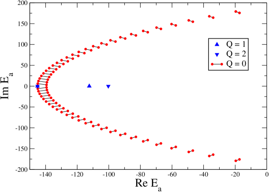
Figure 4: Plot of the roots $\{E_{a}\}_{a=1}^{M}$ of eq.(49) for the three cases described in the text and the values $N=100,M=51,g_{0}=2,h=2$. The roots with $Q_{a}=0,\forall a$ form the “ground state” arc which shrinks when $Q_{1}=1$ or 2 (the roots forming the two arcs are related by the links $\bullet-\bullet$). The real root $\xi_{1}$ for $Q=2$ is close to the bottom of the energy band $\omega=-Nd=-100$. All the energies in figs.4-7 are given in units of $d$.

$Q_{1}/h$	$\xi_{1}^{\rm num}$	$\xi_{1}^{\rm th}$	$\xi_{1}^{\rm th^{\prime}}$	$E$	${E}^{\rm num}_{\rm exc}$	${E}^{\rm th^{\prime}}_{\rm exc}$
3/2	-97.365	-100.021	-100.021	-2694.635	217.998	216.405
1	-100.277	-100.477	-100.481	-2693.203	219.43	216.618
1/2	-112.317	-111.941	-112.059	-2686.975	225.658	222.225
1/3	-132.24	-140.931	-141.476	-2697.788	214.845	238.416

Table 2.- Numerical and theoretical values of the real root $\xi_{1}$, total energy $E$ and excitation energy $E_{\rm exc}=E-E_{0}$ ($E_{0}$ is the ground state energy) for several values of $Q_{1}/h$. The rest of the parameters are fixed to $N=100,M=51,g_{0}=2$. The cases depicted in fig. 4, namely $h=2,Q_{1}=1$ and 2, correspond to the values $Q_{1}/h=0.5$ and 1 in bold face.

Two pairs: Fig. 5-left shows the solutions $E_{a}$ corresponding to two choices: i) $\{Q_{a}=0\}_{a=1}^{M}$ and ii) $Q_{1}=Q_{2}=1$ and $\{Q_{a}=0\}_{a=3}^{M}$ In the second case the roots $E_{1,2}\equiv\xi_{1,2}$ form a complex conjugated pair near the real axis. Observe how the $M$ roots of the ground state arc reorganize themselves into a new arc with two less roots having $Q_{1,2}=1$. In the numerical program one can choose another pair of roots, say $E_{7}$ and $E_{8}$, getting the same result. This is shown in Fig 5-right. In table 3 we collect the numerical and theoretical values for the complex roots $E_{1,2}\equiv\xi_{1,2}$ for several values of the ratio $Q_{1,2}/h$, as well as the excitation energy of the state. The theoretical values will be obtained in the next subsection.

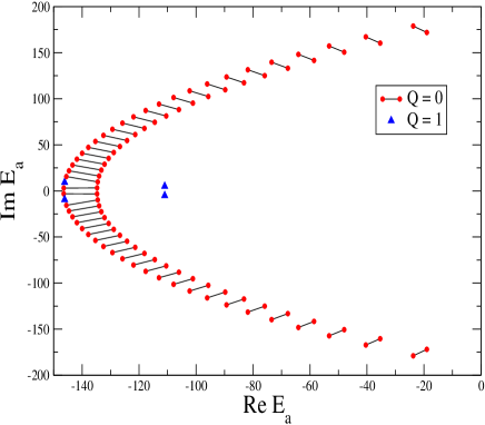
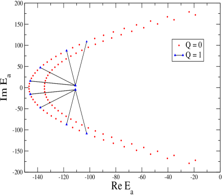
Figure 5: Left: Roots $E_{a}$ of eq.(49) for the values $N=100,M=50,g_{0}=2,h=2$. There are two roots $\xi_{1,2}$ with $Q_{1,2}=1$ forming a complex conjugated pair. Right: Different choices of the roots for which $Q_{a}=1$ yield the same result.

$Q_{1,2}/h$	$\xi^{\rm num}_{1,2}$	$\xi^{\rm th}_{1,2}$	$E$	$E^{\rm num}_{\rm exc}$	${E}^{th}_{\rm exc}$
0.83	$-100.29\pm 1.515\;i$	$-100.092\pm 1.339\;i$	-2481.341	432.458	432.869
0.50	${\bf-111.008\pm 5.058\;i}$	${\bf-110.632\pm 4.963\;i}$	-2470.368	443.431	442.935
0.38	$-126.262\pm 11.498\;i$	$-126.457\pm 8.12\;i$	-2464.325	449.474	459.445

Table 3.- Numerical and theoretical values of the complex roots $E_{1,2}\equiv\xi_{1,2}$, total energy $E$ and excitation energy $E_{\rm exc}$ for several ratios $Q_{1,2}/h$. The rest of the parameters are fixed to $N=100,M=50,g_{0}=2$. The case depicted in fig. 5, namely $h=2,Q_{1,2}=1$, corresponds to the value $Q_{1,2}/h=0.5$ in bold face.

Three pairs: Fig. 6-left shows a solution with three roots formed by a complex pair with $Q_{1,2}=1$ and a real pair with $Q_{3}=2$. In table 4 we collect the results.

$\xi^{\rm num}_{1,2}$	$\xi^{\rm num}_{3}$	$\xi^{\rm th}_{1,2}$	$\xi^{\rm th}_{1,2}$	$E^{\rm num}_{\rm exc}$	${E}^{th}_{\rm exc}$
$-218.229\pm 7.365i$	-201.356	$-222.578\pm 7.115i$	-200.949	1319.06	1320.5

Table 4.- Numerical and theoretical values associated to fig. 6-left.

Five pairs: Fig. 6-right shows a solution with five roots with $Q_{1,\dots,5}=1$, one of which is real and the remaining four are two complex conjugated pairs. As can be seen they form a small arc which one expects to become larger with the number of $Q_{a}=1$ roots.

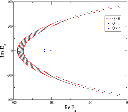
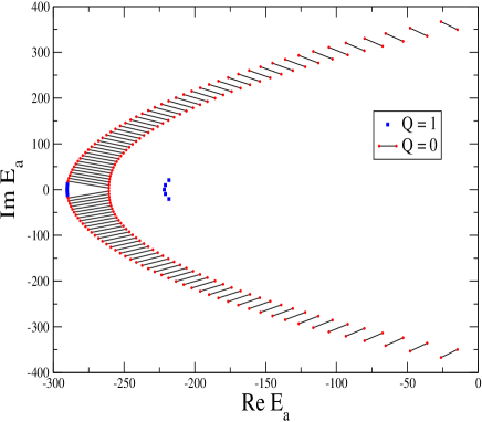
Figure 6: Roots $E_{a}$ of eq.(49) for the cases: Left: $N=200,M=100,g_{0}=2,h=2$. There are two complex roots with $Q_{1,2}=1$ (the closest to the arcs) and a real root with $Q_{3}=2$ (the farther from the arcs). Right: $N=200,M=101,g_{0}=2,h=4$. There are five roots with $Q_{a}=1$.

M/2 pairs: Fig. 7 shows a solution with $M=100$ roots where half of them have $Q_{a}=0$ and the other half have $Q_{a}=1$. This represents a high energy state which is intermediate between the $Q=0$ and $Q=1$ states where all the roots condense into single arcs.

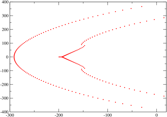
Figure 7: Roots $E_{a}$ of eq.(49) for the values $N=200,M=100,g_{0}=2,h=4$. The wider arc on the LHS is the usual ground state arc. The Y shaped arc in the middle corresponds to $M/2=50$ roots with $Q_{a}=1$, while the two disconnected branches above and below it contain the remaining 50 roots with $Q_{a}=0$.

The main conclusions we can draw from the previous numerical results, and others not shown above, are the following. In the thermodynamic limit where the number of roots $E_{a}$ with $Q_{a}>0$ is kept finite as $N$ and $M$ become very large we have:

• The roots with $Q_{a}=0$ form an open arc $\widetilde{\Gamma}$ which is a slight perturbation of the arc $\Gamma$ formed by the $M$ roots of the ground state.

• The roots with a non vanishing value of $Q_{a}$ fall into arcs characterized by $Q_{a}$.

V.2 Analytic solution

The previous results suggest the steps to follow in the analytical study of eq.(49). We shall employ the methods of complex analysis developed to establish the connection between the Richardson eqs. in the thermodynamic limit and the mean field BCS solution G-book ; largeN (se appendix A for a review).

Let us first rewrite eq.(49) as follows,

$$\sum_{j=1}^{N}{1/2\over\varepsilon_{j}-E_{a}}-\sum_{b=1(\neq a)}^{M}{1\over E_{b}-E_{a}}-{1\over 2G_{a}}=0$$ (50)

where

$${1\over G_{a}}={1\over G_{0}}+{\pi Q_{a}\over\eta},\qquad{1\over G_{0}}={1\over\eta}{\rm Arctan}\left({\eta\over G}\right)$$ (51)

and let us suppose that $Q_{a}=0$ for all roots $E_{a}$ except for a finite number in the limit $N\rightarrow\infty$. We shall call the latter roots $\xi_{\alpha}\;(\alpha=1,\dots,D)$. Making an electrostatic analogy, eqs.(50) and (51) imply that on each root $E_{a}$ acts an electric field $-1/2G_{a}$, which depends on the value of $Q_{a}$. The roots with $Q_{a}=0$ see an electric field $-1/2G_{0}$, while the $Q_{a}>0$ roots see a stronger field. Assuming that all the roots $Q_{a}=0$ form a single arc $\widetilde{\Gamma}$, then the roots $\xi_{\alpha}$, with $Q_{a}>0$, must lie outside $\widetilde{\Gamma}$, namely

$$E_{a}=\left\{\begin{array}[]{cc}\xi\in\widetilde{\Gamma},&Q_{a}=0\\ \xi_{\alpha}\notin\widetilde{\Gamma},&Q_{a}>0\\ \end{array}\right.$$ (52)

There may also exist roots with $Q_{a}=0$ lying outside the arc $\widetilde{\Gamma}$. They will be considered later on. In the continuum limit eqs.(50) split into two sets of eqs. (see appendix A for definitions),

$$\int_{\Omega}{d\varepsilon\;\rho(\varepsilon)\over\varepsilon-\xi}-\sum_{\alpha=1}^{D}{1\over\xi_{\alpha}-\xi}-P\int_{\widetilde{\Gamma}}{|d\xi^{\prime}|\;\widetilde{r}(\xi^{\prime})\over\xi^{\prime}-\xi}-{1\over 2G_{0}}=0,\qquad\xi\in\widetilde{\Gamma},$$ (53)

$$\int_{\Omega}{d\varepsilon\;\rho(\varepsilon)\over\varepsilon-\xi_{\alpha}}-\sum_{\beta=1(\neq\alpha)}^{D}{1\over\xi_{\beta}-\xi_{\alpha}}-P\int_{\widetilde{\Gamma}}{|d\xi^{\prime}|\;\widetilde{r}(\xi^{\prime})\over\xi^{\prime}-\xi_{\alpha}}-{1\over 2G_{\alpha}}=0,\qquad\xi_{\alpha}\notin\widetilde{\Gamma}$$ (54)

where the first equation holds for the roots $\xi$ on the arc $\widetilde{\Gamma}$ and the second equation holds for the roots $\xi_{\alpha}$ outside $\widetilde{\Gamma}$. The density of roots $\widetilde{r}(\xi)$ along the arc $\widetilde{\Gamma}$, and the total energy of the state $E$ are given by (see eqs.(81,82))

$$\int_{\widetilde{\Gamma}}|d\xi|\;\widetilde{r}(\xi)=M-D,$$ (55)

$$\int_{\widetilde{\Gamma}}|d\xi|\;\xi\;\widetilde{r}(\xi)+\sum_{\alpha=1}^{D}\xi_{\alpha}=E.$$ (56)

The solution of eqs.(53,54) follows the same steps as in Appendix A. Let us summarize the results. The density function $\widetilde{r}(\xi)$ can be found from a formula similar to (84) with a modified electric field $\widetilde{h}(\xi)$ given by,

$$\widetilde{h}(\xi)=\widetilde{R}(\xi)\;\left(\int_{\Omega}{\rho(\varepsilon)\over\widetilde{R}(\varepsilon)}\;{d\varepsilon\over\varepsilon-\xi}-\sum_{\alpha=1}^{D}{1\over\widetilde{R}(\xi_{\alpha})(\xi_{\alpha}-\xi)}\right),$$ (57)

with

$$\widetilde{R}(\xi)=\sqrt{(\xi-\widetilde{a})(\xi-\widetilde{b})}$$ (58)

and where $\widetilde{a}=\widetilde{\varepsilon}_{0}-i\widetilde{\Delta},\widetilde{b}=\widetilde{\varepsilon}_{0}+i\widetilde{\Delta}$ are the end points of the arc $\widetilde{\Gamma}$. Using eq.(57) into (53) one gets after some algebra,

$${1\over 2G_{0}}=\int_{\Omega}{d\varepsilon\;\rho(\varepsilon)\over\sqrt{(\varepsilon-\widetilde{\varepsilon}_{0})^{2}+\widetilde{\Delta}^{2}}}-\sum_{\alpha=1}^{D}{1\over\sqrt{(\xi_{\alpha}-\widetilde{\varepsilon}_{0})^{2}+\widetilde{\Delta}^{2}}}$$ (59)

which is a modified gap equation analogous to (91). Similarly (55) gives the modified chemical potential eq. (see (95)),

$$M-D=\int_{\Omega}d\varepsilon\;\rho(\varepsilon)\;\left(1-{\varepsilon-\widetilde{\varepsilon}_{0}\over\sqrt{(\varepsilon-\widetilde{\varepsilon}_{0})^{2}+\widetilde{\Delta}^{2}}}\right)-\sum_{\alpha=1}^{D}\left(1-{\xi_{\alpha}-\widetilde{\varepsilon_{0}}\over\sqrt{(\xi_{\alpha}-\widetilde{\varepsilon}_{0})^{2}+\widetilde{\Delta}^{2}}}\right)$$ (60)

These two equations determine the end points $\widetilde{\varepsilon}_{0}\pm i\widetilde{\Delta}$ of the arc $\widetilde{\Gamma}$. They are formally equivalent to the eqs.(91) and (95) if one defines an effective density

$$\widetilde{\rho}(\varepsilon)=\rho(\varepsilon)+\delta\rho(\varepsilon),\qquad\delta\rho(\varepsilon)=-\sum_{\alpha=1}^{D}\delta(\varepsilon-\xi_{\alpha})$$ (61)

Similarly the eq. (54) for the roots $\xi_{\alpha}$ turns into,

$${\pi Q_{\alpha}\over 2\eta}=\int_{\Omega}d\varepsilon\;{\rho(\varepsilon)\over\varepsilon-\xi_{\alpha}}{\widetilde{R}(\xi_{\alpha})\over\widetilde{R}(\varepsilon)}-\sum_{\beta=1(\neq\alpha)}^{D}{1\over\xi_{\beta}-\xi_{\alpha}}{\widetilde{R}(\xi_{\alpha})\over\widetilde{R}(\xi_{\beta})}+{\widetilde{R^{\prime}}(\xi_{\alpha})\over\widetilde{R}(\xi_{\alpha})}$$ (62)

where the RHS can be identified with the electric field $\widetilde{h}(\xi_{\alpha})$ (see eq.(57)), after subtracting the pole at $\xi=\xi_{\alpha}$. Finally, the energy of the state can be derived from eq.(56) and it reads,

$$E = -{\widetilde{\Delta}^{2}\over 4G_{0}}+\int_{\Omega}d\varepsilon\;\varepsilon\;\left(1-{\varepsilon-\widetilde{\varepsilon}_{0}\over\sqrt{(\varepsilon-\widetilde{\varepsilon}_{0})^{2}+\widetilde{\Delta}^{2}}}\right)\rho(\varepsilon)$$

$$+\sum_{\alpha=1}^{D}\xi_{\alpha}-\sum_{\alpha=1}^{D}\xi_{\alpha}\left(1-{\xi_{\alpha}-{\widetilde{\varepsilon}_{0}}\over\sqrt{(\xi_{\alpha}-\widetilde{\varepsilon}_{0})^{2}+\widetilde{\Delta}^{2}}}\right)$$

Doing a computation similar to the one that leads to eqs.(101) and (Appendix B: Elementary excitations of BCS in the canonical ensemble) in Appendix B one gets the excitation energy of the state $E_{exc}=E-E_{0}$ ($E_{0}$ is the ground state energy)

$$E_{exc}=\sum_{\alpha=1}^{D}\sqrt{(\xi_{\alpha}-\varepsilon_{0})^{2}+\Delta^{2}}\;,$$ (64)

where $\Delta$ and $\varepsilon_{0}$ are the unperturbed values of the gap and chemical potentials given by the solution of eqs.(91) and (95) with $G=G_{0}$.

V.3 Analytic versus numerics

Let us compare the analytic and the numerical results obtained previously. For one real pair $\xi_{1}$ the eq.(62) becomes,

$${\pi Q_{1}\over 2\eta}=\int_{\Omega}d\varepsilon\;{\rho(\varepsilon)\over\varepsilon-\xi_{1}}{\widetilde{R}(\xi_{1})\over\widetilde{R}(\varepsilon)}+{\widetilde{R^{\prime}}(\xi_{1})\over\widetilde{R}(\xi_{1})}$$ (65)

In the large N limit we can approximate $\widetilde{R}(\xi)$ by $R(\xi)$, so that (65) simplifies,

$${\pi Q_{1}\over 2\eta}=h(\xi_{1})+{\xi_{1}-\varepsilon_{0}\over(\xi_{1}-\varepsilon_{0})^{2}+\Delta^{2}}$$ (66)

where we have used (93). In the equally spaced model at half filling the integral giving $h(\xi)$ is given by the formula largeN ,

$$h(\xi)={1\over 4d}\;\log{{(\xi-\omega)(\Delta^{2}-\xi\omega+\sqrt{(\Delta^{2}+\xi^{2})(\Delta^{2}+\omega^{2})})\over(\xi+\omega)(\Delta^{2}+\xi\omega+\sqrt{(\Delta^{2}+\xi^{2})(\Delta^{2}+\omega^{2})})}}\;.$$ (67)

To compare with the numerical results collected in table 2 we solve eq.(66) for the values, $N=100,\;g_{0}=2,\;d=1$ which implies that $\Delta=Nd/\sinh(1/g_{0})=191.903$, $\varepsilon_{0}=0$ and $\omega=dN=100$. The result is given in table 2 in the column $\xi_{1}^{\rm th^{\prime}}$. The excitation energy is obtained using (64), namely $E_{\rm exc}=\sqrt{(\xi_{1}^{\rm th^{\prime}})^{2}+\Delta^{2}}$ and the values appear in the column $E^{\rm th^{\prime}}_{\rm exc}$ of table 2. Observe the good agreement between the numerical and theoretical values.

As can be seen from eq.(67) the field $h(\xi_{1})$ is proportional to $1/d\sim N$, hence in the large N limit the eq. (66) can be approximated by

$${\pi Q_{1}\over 2\eta}=h(\xi_{1})$$ (68)

On the other hand the change of variables largeN

$$\xi={i\Delta\cosh u\over\sqrt{1-\left({\Delta\over\omega}\sinh u\right)^{2}}}$$ (69)

leads to a very simple expression for $h(\xi)$, namely

$$h(\xi)=-{u\over 2d}$$ (70)

So that the solution of eq.(68) is given simply by

$$\xi_{1}=-{\Delta\cosh(\pi Q/h)\over\sqrt{-1+\left({\Delta\over\omega}\sinh(\pi Q/h)\right)^{2}}}$$ (71)

The column $\xi_{1}^{\rm th}$ of table 2 collects several values of (71), which are quite close to the values of $\xi_{1}^{\rm th^{\prime}}$. The solution (71) remains real and below the bottom of the band, i.e. $\xi_{1}<-\omega$, whenever $\pi Q/h>1/g_{0}$.

To check the results of table 3 one has to solve eq.(62) for two complex roots, say $\xi_{1}$ and $\xi_{2}=\xi_{1}^{*}$ with $Q_{1}=Q_{2}$,

$${\pi Q_{1}\over 2\eta}=h(\xi_{1})-{1\over\xi_{2}-\xi_{1}}{R(\xi_{1})\over R(\xi_{2})},\qquad{\pi Q_{2}\over 2\eta}=h(\xi_{2})-{1\over\xi_{1}-\xi_{2}}{R(\xi_{2})\over R(\xi_{1})}$$ (72)

Notice that we drop the term $R^{\prime}(\xi)/R(\xi)$ in these equations. The numerical results are shown in the column $\xi^{\rm th}_{1,2}$. Similarly the excitation energy is given by $E_{\rm exc}=2Re[\sqrt{(\xi_{1}^{\rm th})^{2}+\Delta^{2}}]$ Finally, the theoretical results of table 4 are obtained by choosing $\xi_{1,2}^{\rm th}$ as the solutions of eqs.(72), and $\xi_{3}^{\rm th}$ from eq.(71). Strictely speaking one must solve eqs.(62) for three roots with $Q_{a}=1,1,2$, but they can be approximated as above. The energy is given by (64) summing over the three roots $\xi_{i}^{\rm th}$.

V.4 The $Q$-excitations in the PBCS ansatz

Let us summarize the results obtained so far. Using the grand canonical BCS ansatz we showed the existence of different solutions of the gap equation in the RD model characterized by an integer $Q\geq 0$, where the $Q=0$ solution corresponds to the ground state and the solutions with $Q\geq 1$ correspond to higher excited states with different condensation energies. Later on, the exact solution of the model led us to identify the integer $Q$ with the Bethe numbers appearing in the solution of the BAE for the $M$ roots, namely $Q=Q_{a},\;\forall a$. This suggested the existence of low lying excited states for which $Q_{a}=0$ for most of the roots, in the thermodynamic limit, except for a finite number of them, for which $Q_{a}\geq 1$. These new type of excitations cannot be derived from the standard mean field analysis in the grand canonical ensemble which are given in terms of the familiar Bogoliubov quasiparticles. This is why we have to use the exact solution to find them. One may wonder however if there is an alternative way to derive the $Q-$excitations, which could be valid in more general circumstances. We now argue that this is indeed possible using the projected BCS ansatz. Let us write the BCS state defined in eq.(3) as

$$|\psi_{0}\rangle\propto{\rm exp}\left(\sum_{k}g_{k}b^{\dagger}_{k}\right)\;|0\rangle$$ (73)

where $g_{k}=v_{k}/u_{k}$ is the wave function of the Cooper pair in momentum space. A state with $M$ pairs can be obtained from (73) keeping the $M^{\rm th}$-term of the Taylor expansion, i.e.

$$|M\rangle\propto\left(\sum_{k}g_{k}b^{\dagger}_{k}\right)^{M}\;|0\rangle$$ (74)

which is called the Projected BCS state (PBCS). While the grand canonical BCS state (73) is an eigenstate of the phase operator we see that (74) is an eigenstate of the electron number operator. In the large $N$ limit the results obtained with both ansatze agree to leading order in $N$. However for finite values of $N$ the BCS and PBCS give different results as ocurred when they were applied to the study of ultrasmall superconducting grains BvD ; DMRG1 ; DMRG2 . In the RD model the PBCS state corresponding to the $Q^{\rm th}$-solution can be written as

$$|M_{Q}\rangle\propto\left(\sum_{k}g_{k}^{(Q)}b^{\dagger}_{k}\right)^{M_{Q}}\;|0\rangle$$ (75)

where $g^{(Q)}_{k}$ is the associated wave function. The ground state is given by (75) with $Q=0$. We shall conjecture that the states found in the subsections V-A and V-B can be approximated by the following PBCS states

$$|M_{0},M_{1},\dots\rangle\propto\left(\sum_{k}g_{k}^{(0)}b^{\dagger}_{k}\right)^{M_{0}}\left(\sum_{k}g_{k}^{(1)}b^{\dagger}_{k}\right)^{M_{1}}\dots\;|0\rangle$$ (76)

where $M_{0}\sim{\cal O}(M)$ is the number of roots with $Q_{a}=0$, $M_{1}\sim{\cal O}(1)$ the number of roots with $Q_{a}=1$, etc. Eq.(76) certainly holds in the case where the operators $b_{k}$ are ordinary bosons instead of hard core ones. In this case the RD Hamiltonian can be diagonalized by a canonical transformation of the boson operators $b_{k}$ which amounts to solving the BAE for one pair, eq.(32). Each term in (76) would correspond to the bound state solutions of the one pair problem with $Q=0,1,\dots$.

An important consequence of this discussion is that the Q-excitations must behave as ordinary bosons. In the canonical picture one simply adds one more pair to the $Q>0$ states, which then increases the excitation energy. In the exact solution this corresponds to removing pairs from the ground state arc and place them into the small arcs with $Q_{a}>0$. This property is in sharp contrast with the standard quasiparticles which are fermions.

V.5 Pair-hole excitations as $Q_{a}=0$ states

So far we have considered the solutions of eq.(49) where some of the $Q_{a}$ are non zero which has the effect that the associated roots come out from the ground state arc. In excita it was shown that the Richardson eqs. (27) already contains many solutions where this happens. The latter solutions correspond to the pair-hole excitations of the BCS model, to be distinguished from the excitations where the energy levels are blocked by single electrons. (see appendix B). In the large $N$ limit the pair-hole excitations are characterized by the fact that $N_{G}$ roots $E_{a}$ lie outside the arc $\widetilde{\Gamma}$ formed by the $M-N_{G}$ remaining ones excita . In figure 8 we show an example of two excited states with $N_{G}=1$ and 2 roots for a model with $M=20$ roots. Figure 8a is similar to fig.4 since in both cases one root comes out of the ground state arc $\Gamma$. They differ however in the value of $Q_{1}$, which is 1 in fig. 4 and 0 in fig. 8a. In excita it was found that the roots $E_{\alpha}\;(\alpha=1,\dots,N_{G})$, lying outside the arc $\widetilde{\Gamma}$ satisfy in the large $N$ limit the following eq.

$$0=\int_{\Omega}d\varepsilon\;{\rho(\varepsilon)\over\varepsilon-\xi_{\alpha}}{\widetilde{R}(\xi_{\alpha})\over\widetilde{R}(\varepsilon)}-\sum_{\beta\neq\alpha}^{N_{G}}{1\over(\xi_{\beta}-\xi_{\alpha})}{R(\xi_{\alpha})\over R(\xi_{\beta})}+{R^{\prime}(\xi_{\alpha})\over R(\xi_{\alpha})}\;,$$ (77)

which coincides with eq.(62) upon the choice $Q_{\alpha}=0$. Moreover the energy of these excited states is given by,

$$E_{exc}=\sum_{\alpha=1}^{N_{G}}\sqrt{(\xi_{\alpha}-\varepsilon_{0})^{2}+\Delta^{2}}\;,$$ (78)

This formula coincides with eq.(64) giving the energy of the $Q_{a}$-excitations. Hence the pair-hole excitations of excita can be seen as $Q_{a}=0$ excitations.

Summarizing, in the RD model there are three types of excitations in the canonical ensemble, i) the ones obtained by the blocking of energy levels, ii) the pair-hole excitations and iii) the $Q-$excitations. The first two have already been considered for the standard BCS model and in the g.c. ensemble they correspond to the quasiparticles which have fermionic statistics. The last ones are specific of the RD model and have bosonic statistics. These results must have profound consequences in the thermodynamical properties of the system and its response to external fields.

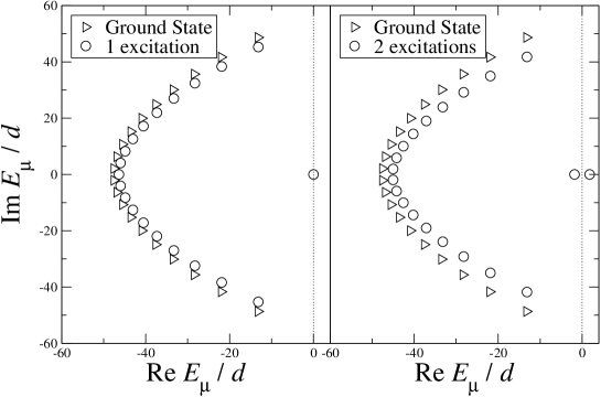
Figure 8: Position $M=20$ pairs of the states at $g=1.5$. The arcs $\widetilde{\Gamma}$ for 19 pairs (left) and 18 pairs (right) are a slight modification of the ground state arc $\Gamma$ (20 pairs) excita .

VI Conclusions and prospects

In this paper we have analyzed in more depth the Russian doll BCS model using its exact solution. We have shown that the mean field solution obtained in RD agrees in the limit of large number of particles $N$ with the exact solution to leading order in $N$. In doing so we have identified the integer $Q$, that labels the mean field solutions, with the Bethe numbers appearing in the BAE. This integer also has a RG meaning since it counts the number of RG cycles. This idea is clarified by deriving the BAE for one Cooper pair using the RG method of Glazek and Wilson GW . The numerical solution of the latter equation shows the appearance of bound states with $Q>0$ and of unbounded states with $Q<0$. We have also studied the many body case in the large $N$ limit, where the BAE can be approximated by Richardson like equations where the value of the effective BCS coupling constant depends on the Bethe numbers $Q_{a}$. We have solved numerically and analytically these equations showing the existence of solutions where the Bethe numbers $Q_{a}$ may vary with the roots. The most interesting case is when $Q_{a}$ vanishes for most of the roots except for a small number where they are positive. These solutions correspond to low energy excitations where Cooper pairs, forming the ground state, jump into excited states characterized by positive values of $Q_{a}>0$. In this sense $Q_{a}$ becomes a sort of principal quantum number of the Cooper pairs. These new type of elementary excitations should be added to the standard ones to describe the low energy spectrum of the model, whose thermodynamical properties and response to external fields will be modified.

Acknowledgments. We would like to thank J.M. Román, J. Dukelsky, G. Morandi and M. Roncaglia for discussions. This work is supported by the grants FIRB 2002-2005 project number RBAU018472 of Italian MIUR (AA), the NSF of the USA (AL) and the CICYT of Spain under the contract BFM2003-05316-C02-01 (GS). We also thank the EC Commission for financial support via the FP5 Grant HPRN-CT-2002-00325.

Appendix A: Gaudin’s electrostatic solution of Richardson equations

In this section we review the electrostatic method employed by Gaudin in the proof of the asymptotic agreement of the exact and mean field solutions G-book (see also largeN ; amico-electro ). The starting point of Gaudin’s approach is the observation that the Richardson eq.(27), that we shall rewrite as

$$\sum_{j=1}^{N}{1/2\over\varepsilon_{j}-E_{a}}-\sum_{b=1(\neq a)}^{M}{1\over E_{b}-E_{a}}-{1\over 2G}=0$$ (79)

can be seen as the equilibrium conditions for a set of mobile charges $+1$ located at the positions $E_{a}$ in the complex plane under the effect of a constant electric field $-1/2G$ and another set of charges $-1/2$ at the positions $\varepsilon_{j}$. In the large $N$ limit the pair energy levels $\varepsilon_{j}$ will be equivalent to a negative charge density $-\rho(\varepsilon)$ located on an interval $\Omega=(-\omega,\omega)$ of the real axis. The total charge of this interval is given by

$$-\int_{\Omega}d\varepsilon\;\rho(\varepsilon)=-{N\over 2}\;,\qquad\rho(\varepsilon)={1\over 2}\sum_{j=1}^{N}\delta(\varepsilon-\varepsilon_{j})$$ (80)

The numerical solutions of eqs. (79) are either real or complex roots in which case they come in conjugated pairs R-roots ; largeN . In the large $N$ limit the complex roots form an open arc $\Gamma$ whose end points are given by $a=\varepsilon_{0}-i\Delta$ and $b=\varepsilon_{0}+i\Delta$, where $\varepsilon_{0}$ is the chemical potential and $\Delta$ is the gap (see fig. 9). Let us assume for simplicity that all the roots are complex. We shall call $r(\xi)$ the linear charge density of roots $E_{a}$ along the arc $\Gamma$. Hence, the total number of pairs, $M$, and energy, $E$, are given by

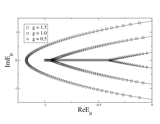
Figure 9: Plot of the roots $E_{\mu}$ for the equally spaced model in the complex plane (taken from largeN ). The discrete symbols denote the numerical values for $M=100$. The continuous lines are the analytical curves obtained in largeN . All the energies are in units of $\omega$.

$$\int_{\Gamma}|d\xi|\;r(\xi) = M,$$ (81)

$$\int_{\Gamma}|d\xi|\;\xi\;r(\xi) = E.$$ (82)

The continuum limit of eqs. (79) is

$$\int_{\Omega}{d\varepsilon\;\rho(\varepsilon)\over\varepsilon-\xi}-P\int_{\Gamma}{|d\xi^{\prime}|\;r(\xi^{\prime})\over\xi^{\prime}-\xi}-{1\over 2G}=0,\qquad\xi\in\Gamma,$$ (83)

which implies the vanishing of the total electric field on every point of the arc $\Gamma$. The solution of eqs. (83) can be found as follows. First of all, let us orient the arc $\Gamma$ from the point $a$ to the point $b$, and call $L$ an anticlockwise path encircling $\Gamma$. We look for an analytic field $h(\xi)$ outside $\Gamma$ and the set $\Omega$, such that

$$r(\xi)\;|d\xi|={1\over 2\pi i}(h_{+}(\xi)-h_{-}(\xi))\;d\xi,\qquad\xi\in\Gamma,$$ (84)

where $h_{+}(\xi)$ and $h_{-}(\xi)$ denote the limit values of $h(\xi)$ to the right and left of $\Gamma$. This can be understood using the electrostatic equivalence, considering that the electric field presents a discontinuity proportional to the linear charge density when crossing the arc $\Gamma$. Next, we define a function $R(\xi)$, with cuts along the curve $\Gamma$, by the equation

$$R(\xi)=\sqrt{(\xi-a)(\xi-b)},$$ (85)

and look for a solution which vanishes at the boundary points of $\Gamma$, in the form

$$h(\xi)=R(\xi)\;\int_{\Omega}{d\varepsilon\;\varphi(\varepsilon)\over\varepsilon-\xi}\;.$$ (86)

This field has to be constant at infinity, as can be verified explicitly. The contour integral surrounding the charge density $r(\xi)$ in (83) can be expressed as

$$\int_{\Gamma}{|d\xi^{\prime}|\;r(\xi^{\prime})\over\xi-\xi^{\prime}}={1\over 2\pi i}\int_{\Gamma}d\xi^{\prime}\;{h_{+}(\xi^{\prime})-h_{-}(\xi^{\prime})\over\xi-\xi^{\prime}}={1\over 2\pi i}\int_{L}d\xi^{\prime}\;{h(\xi^{\prime})\over\xi-\xi^{\prime}},\qquad\xi\in{\bf C}\Gamma,$$ (87)

where ${\bf C}\Gamma$ is the region outside the curve $\Gamma$. Using eqs. (85) and (86), one finds for the principal value of (87)

$$P\int_{\Gamma}{|d\xi^{\prime}|\;r(\xi^{\prime})\over\xi-\xi^{\prime}}={1\over 2\pi i}\int_{L}{d\xi^{\prime}R(\xi^{\prime})\over\xi-\xi^{\prime}}\int_{\Omega}{d\varepsilon\;\varphi(\varepsilon)\over\varepsilon-\xi^{\prime}}=-\int_{\Omega}d\varepsilon\;{\varphi(\varepsilon)R(\varepsilon)\over\varepsilon-\xi}+\int_{\Omega}d\varepsilon\;\varphi(\varepsilon),\qquad\xi\in\Gamma,$$ (88)

where we have deformed the contour of integration $L$ into two contours, one encircling the interval $\Omega$ (first term on the RHS) and another one around the infinity (second term). We are assuming that $\Gamma$, and consequently $L$, do not cut the interval $\Omega$, which happens int the equally spaced model when $g>g_{c}=1.13459$ largeN . Plugging eq. (88) into (83), we see that a solution is obtained provided

$$\varphi(\varepsilon)={\rho(\varepsilon)\over R(\varepsilon)},$$ (89)

$$\int_{\Omega}d\varepsilon\;{\rho(\varepsilon)\over R(\varepsilon)}={1\over 2G}\;,$$ (90)

Using (85) the eq.(90) becomes,

$$\int_{\Omega}{d\varepsilon\;\rho(\varepsilon)\over\sqrt{(\varepsilon-\varepsilon_{0})^{2}+\Delta^{2}}}={1\over 2G}\;.$$ (91)

which is nothing but the BCS gap eq.(9) in the appropriate normalizations (see eq.(97) below). The field $h(\xi)$ gives the charge density $r(\xi)$,

$$r(\xi)={1\over\pi}|h(\xi)|\;,\qquad\xi\in\Gamma,$$ (92)

and its value is given by replacing (89) into (86), i.e.

$$h(\xi)=R(\xi)\;\int_{\Omega}{\rho(\varepsilon)\over R(\varepsilon)}\;{d\varepsilon\over\varepsilon-\xi}\;,$$ (93)

The equation fixing the arc $\Gamma$ are the equipotential curves of the total distribution,

$${\cal R}\int_{a}^{\xi}d\xi^{\prime}\;h(\xi^{\prime})=0,\qquad\xi\in\Gamma.$$ (94)

Similarly, eq. (81) becomes the chemical potential equation

$$M={1\over 2\pi i}\int_{L}d\xi\;h(\xi)=\int_{\Omega}d\varepsilon\;\rho(\varepsilon)\;\left(1-{\varepsilon-\varepsilon_{0}\over\sqrt{(\varepsilon-\varepsilon_{0})^{2}+\Delta^{2}}}\right),$$ (95)

while eq. (82) gives the BCS expression for the ground state energy,

$$E={1\over 2\pi i}\int_{L}d\xi\;\xi\;h(\xi)=-{\Delta^{2}\over 4G}+\int_{\Omega}d\varepsilon\;\varepsilon\;\left(1-{\varepsilon-\varepsilon_{0}\over\sqrt{(\varepsilon-\varepsilon_{0})^{2}+\Delta^{2}}}\right)\rho(\varepsilon).$$ (96)

Comparing these equations with the corresponding ones in the BCS theory, we deduce the following relations between $\Delta$, $\varepsilon_{0}$, and $\rho(\varepsilon)$, and $\Delta_{BCS}$ (BCS gap), $\mu$ (chemical potential), and $n(\epsilon)$ (single particle energy density):

$$\Delta=2\Delta_{BCS},\qquad\varepsilon_{0}=2\mu,\qquad\rho(\varepsilon)={1\over 4}\;n\left({\varepsilon\over 2}\right).$$ (97)

Appendix B: Elementary excitations of BCS in the canonical ensemble

In the grand canonical ensemble the excited states can be obtained acting on the GS ansatz $|\psi_{0}\rangle$ with the Bogoliubov operators $\gamma_{j,\sigma}\;(\sigma=\pm)$

$$\gamma_{j_{1},\sigma_{1}}\dots\gamma_{j_{n},\sigma_{n}}|\psi_{0}\rangle,\qquad\gamma_{j,\pm}=u_{j}\,c_{j\pm}\mp v_{j}\,c^{\dagger}_{j\mp},$$ (98)

where the variational parameters $u_{j},v_{j}$ are given by eqs. similar to (4). The excitation energy is given by (recall the factor of 2 in our conventions as compare to the standard ones).

$$E_{exc}=E-E_{0}={1\over 2}\sum_{j}\sqrt{(\varepsilon_{j}-\varepsilon_{0})^{2}+\Delta^{2}}$$ (99)

We have to distinguish between two sorts of excitations: E1) quasiparticles occupying different energy levels, which means that all the $j^{\prime}s$ in eq. (98) are different, and E2) quasiparticles occupying the same energy level, i.e. $\gamma^{\dagger}_{j,+}\gamma^{\dagger}_{j,-}$. In the latter case the factor $(u_{j}+v_{j}\,b^{\dagger}_{j})$ in the ground state is replaced by the factor $(v_{j}-u_{j}\,b^{\dagger}_{j})$. The states E2 are called “real pairs” to be distinguished from the “virtual pairs” that build up the ground state BCS-book

In the canonical ensemble the Bogoliubov operators do not even make sense since they change the particle number which is fixed by definition. It is however possible to see the correspondence of these excitations in the canonical ensemble. The excitations of type E1 correspond to blocking of energy levels and we discuss them next in detail. The excitation of type E2 correspond to pair-hole excitations and they are discussed in subsection V-E.

Blocking of energy levels

Let us break $P$ pairs of the $M$ pairs forming the ground state and place the corresponding $2P$ electrons in different $2P$ levels belonging to the set $B=\{j_{1}<j_{2}<\dots<j_{2P}\}$. All these levels are singly occupied and therefore the corresponding electrons decouple from the rest of the system contributing only with their free kinetic energy ${1\over 2}\,\varepsilon_{j},\;j\in B$. The remaining $M-P$ pairs are then allowed to occupy the $N-2P$ energy levels that are left (see fig. 10 for an example).

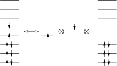
Figure 10: Excited state obtained by breaking a “Cooper pair” at $G=0$. On the RHS the singly occupied levels are blocked and decouple from the rest of the system.

The problem we are left with is entirely similar to the original one after removing the blocked levels. This is turn is equivalent to consider the modified density of levels,

$$\widetilde{\rho}(\varepsilon)=\rho(\varepsilon)+\delta\rho(\varepsilon),\qquad\delta\rho(\varepsilon)=-{1\over 2}\sum_{j\in B}\delta(\varepsilon-\varepsilon_{j})$$ (100)

where $\rho(\varepsilon)$ was defined in (80). This small perturbation of $\rho(\varepsilon)$ translates into a small perturbation of the density, i.e. $\widetilde{r}(\xi)=r(\xi)+\delta r(\xi)$ and that of the arc $\Gamma$ whose ends points will move slightly, i.e. $\widetilde{\varepsilon}_{0}=\varepsilon_{0}+\delta\varepsilon_{0}$ and $\widetilde{\Delta}=\Delta+\delta\Delta$. The eqs. for the deviations in the chemical potential and the gap can be obtained by taking the variation of the gap eq.(91) and the chemical potential eq.(95):

$$\int_{\Omega}d\varepsilon\;{\rho(\varepsilon)\over R(\varepsilon)^{3}}\;\left[\Delta\delta\Delta-(\varepsilon-\varepsilon_{0})\delta\varepsilon_{0}\right] = \int_{\Omega}d\varepsilon\;{\delta\rho(\varepsilon)\over R(\varepsilon)}$$ (101)

$$\int_{\Omega}d\varepsilon\;{\rho(\varepsilon)\Delta\over R(\varepsilon)^{3}}\;\left[(\varepsilon-\varepsilon_{0})\delta\Delta+\Delta\delta\varepsilon_{0}\right] = \delta M-\int_{\Omega}d\varepsilon\;\delta\rho\left(1-{\varepsilon-\varepsilon_{0}\over R(\varepsilon)}\right)$$

where $R(\varepsilon)$ is given by eq.(85). Taking the variation in (96) one finds

$$\delta E = -{\Delta\delta\Delta\over 2G}+\int_{\Omega}d\varepsilon\;\varepsilon\;{\rho(\varepsilon)\Delta\over R(\varepsilon)^{3}}\left[(\varepsilon-\varepsilon_{0})\delta\Delta+\Delta\delta\varepsilon_{0}\right]$$

$$+\int_{\Omega}d\varepsilon\;\varepsilon\;\delta\rho(\varepsilon)\left(1-{\varepsilon-\varepsilon_{0}\over R(\varepsilon)}\right)$$

Using the gap eq. for the first term in the RHS and applying the eqs. (101) one gets,

$$\delta E = \varepsilon_{0}\delta M+\int_{\Omega}d\varepsilon\;\delta\rho(\varepsilon)\;\left[\varepsilon-\varepsilon_{0}-R(\varepsilon)\right]$$

$$= {1\over 2}\sum_{j\in B}(R(\varepsilon_{j})-\varepsilon_{j})$$

where we used (100) and $\delta M=-P$. We have to add to eq.(Appendix B: Elementary excitations of BCS in the canonical ensemble) the contribution of the single occupied levels, namely ${1\over 2}\sum_{j\in B}\varepsilon_{j}$ which then coincides with the Bogoliubov formula (99). This proves the one to one correspondence between the Bogoliubov quasiparticles occupying different energy levels and the blocked levels in the canonical ensemble.

References

- (1) K. G. Wilson, “Renormalization Group and Strong Interactions”, Phys. Rev. D3 (1971) 1818.
- (2) P. F. Bedaque, H.-W. Hammer, and U. van Kolck, “Renormalization of the Three-Body System with Short-Range Interactions”, Phys. Rev. Lett. 82 (1999) 463, nucl-th/9809025.
- (3) D. Bernard and A. LeClair, “Strong-weak coupling duality in anisotropic current interactions”, Phys.Lett. B512 (2001) 78; hep-th/0103096.
- (4) A. LeClair, J.M. Román and G. Sierra, “Russian Doll Renormalization Group and Kosterlitz-Thouless Flows”, Nucl. Phys. B675 (2003) 584; hep-th/0301042.
- (5) S. D. Glazek and K. G. Wilson, “Limit cycles in quantum theories”, Phys. Rev. Lett. 89 (2002) 230401, hep-th/0203088; “Universality, marginal operators, and limit cycles”, cond-mat/0303297.
- (6) A. LeClair, J.M. Román and G. Sierra, “Russian Doll Renormalization Group and Superconductivity”, Phys. Rev. B69 (2004) 20505 (R); cond-mat/0211338.
- (7) A. LeClair, J.M. Román, G. Sierra, “Log-periodic behaviour of finite size effects in field theory models with cyclic renormalization group”, Nucl. Phys. B700 (2004) 407-435; hep-th/0312141.
- (8) A. LeClair and G. Sierra, “Renormalization group limit-cycles and field theories for elliptic S-matrices”, J. Stat. Mech.: Theor. Exp. (2004) P08004; hep-th/0403178.
- (9) E. Braaten, H.-W. Hammer, and M. Kusunoki, “Efimov States in a Bose-Einstein Condensate near a Feshbach Resonance”, Phys. Rev. Lett. 90 (2003) 170402, cond-mat/0206232.
- (10) E. Braaten and H.-W. Hammer, “An Infrared Renormalization Group Limit Cycle in QCD”, Phys. Rev. Lett. 91 (2003) 102002, nucl-th/0303038.
- (11) E. Braaten and H.-W. Hammer, “ Universality in Few-body Systems with Large Scattering Length”, cond-mat/0410417.
- (12) I.R. Klebanov and M. J. Strassler, “Supergravity and a Confining Gauge Theory: Duality Cascades and SB-Resolution of Naked Singularities”, JHEP 0008 (2000) 052, hep-th/0007191.
- (13) A. Morozov and A. J. Niemi, “Can Renormalization Group Flow End in a Big Mess?”, Nucl.Phys. B666 (2003) 311, hep-th/0304178.
- (14) M. Tierz, “Quantum group symmetry and discrete scale invariance: Spectral aspects”, hep-th/0308121.
- (15) J. Bardeen, L.N. Cooper and J.R. Schrieffer, “Theory of Superconductivity”, Phys. Rev. 108, 1175 (1957).
- (16) J.R. Schrieffer, “Theory of Superconductivity”, Frontiers in Physics, Addison-Wesley Pub., New York (1988).
- (17) C. Dunning and J. Links, “Integrability of the Russian doll BCS model”, Nucl. Phys. B702 (2004) 481, cond-mat/0406234.
- (18) D.C. Ralph, C.T. Black and M. Tinkham, “Spectroscopy of the superconducting gap in individual nanometer-scale aluminum particles”, Phys. Rev. Lett. 76, 688 (1996); “Gate-voltage studies of discrete electronic states in aluminum nanoparticles”, Phys. Rev. Lett. 78, 4087 (1997).
- (19) J. von Delft and D. C. Ralph, “Spectroscopy of discrete energy levels in ultrasmall metallic grains”, Physics Reports, 345, 61 (2001), cond-mat/0101019.
- (20) R. W. Richardson, “A restricted class of exact eigenstates of the pairing-force Hamiltonian”, Phys. Lett. 3, (1963) 277.
- (21) R.W. Richardson and N. Sherman, “Exact eigenstates of the pairing-force Hamiltonian”, Nucl. Phys. B 52 (1964) 221.
- (22) R.W. Richardson, “Numerical study of 8-32 particle eigenstates of pairing Hamiltonian”, Phys. Rev. 141, 949 (1966).
- (23) M.C. Cambiaggio, A.M.F. Rivas and M. Saraceno, “Integrability of the pairing Hamiltonian”, Nucl. Phys. A 624, 157 (1997).
- (24) J. Dukelsky, S. Pittel and G. Sierra, “Exactly solvable Richardson-Gaudin models for many-body quantum systems”, Rev. Mod. Phys. 76 (2004) 643-662; nucl-th/0405011.
- (25) L. Amico, G. Falci and R. Fazio, “The BCS model and the off shell Bethe ansatz for vertex models”, J.Phys. A 34 (2001) 6425, cond-mat/0010349.
- (26) H.-Q. Zhou, J. Links, R.H. McKenzie and M.D. Gould, “Superconducting correlations in metallic nanoparticles: exact solution of the BCS model by the algebraic Bethe ansatz”, Phys. Rev. B 56 (2002) 060502(R), cond-mat/0106390. cond-mat/0106390.
- (27) J. von Delft and R. Poghossian, “Algebraic Bethe Ansatz for a discrete-state BCS pairing model”, Phys. Rev. B 66, 134502 (2002), cond-mat/0106405.
- (28) G. Sierra, “Integrability and Conformal Symmetry in the BCS model”, in Proceedings of the NATO Advanced Research Workshop on Statistical Field Theories, Como, Italy, June 2001. Eds. A. Cappelli y G. Mussardo. Kluwer Academic Publishers, 2002, The Netherlands. hep-th/0111114.
- (29) L.D. Faddeev, “How Algebraic Bethe Ansatz works for integrable model”, Les-Houches Lectures, hep-th/9605187.
- (30) M. Gaudin, “ États propres et valeurs propres de l’Hamiltonien d’appariement”, unpublished Saclay preprint, 1968. Included in Travaux de Michel Gaudin, Modèles exactament résolus, Les Éditions de Physique, France, 1995.
- (31) R.W. Richardson, “Pairing in the limit of a large number of particles”, J. Math. Phys. 18, 1802 (1977).
- (32) J.M. Román, G. Sierra, J. Dukelsky, “Large N limit of the exactly solvable BCS model: analytics versus numerics”, Nucl. Phys. B634 (2002) 483; cond-mat/0202070.
- (33) R. Hernandez, E. Lopez, A. Perianez and G. Sierra, “Finite size effects in ferromagnetic spin chains and quantum corrections to classical strings”; hep-th/0502188.
- (34) Fabian Braun and J. von Delft, “ Fixed-N Superconductivity: The Crossover from the Bulk to the Few-Electron Limit”, Phys. Rev. Lett. 81, 4712 (1998), cond-mat/9810146.
- (35) J. Dukelsky and G. Sierra, “A Density Matrix Renormalization Group Study of Ultrasmall Superconducting Grains”, Phys. Rev. Lett. 83, 172 (1999), cond-mat/9903332.
- (36) J. Dukelsky and G. Sierra, “The Crossover from the Bulk to the Few-Electron limit in Ultrasmall Metallic Grains” Phys. Rev. B 61, 12302 (2000), cond-mat/9906166.
- (37) J.M. Román, G. Sierra and J. Dukelsky, “Elementary excitations of the BCS model in the canonical ensemble”, J.M. Román, G. Sierra, J. Dukelsky, Phys. Rev. B 67, 64510 (2003); cond-mat/0207640.
- (38) L. Amico, A. Di Lorenzo, A. Mastellone, A. Osterloh, R. Raimondi, “Electrostatic analogy for integrable pairing force Hamiltonians”, Annals Phys. 299 (2002) 228-250; cond-mat/0204432.