Temperature Cycles in the Heisenberg Spin Glass

Abstract

We study numerically the nonequilibrium dynamics of the three-dimensional Heisenberg Edwards-Anderson spin glass submitted to protocols during which temperature is shifted or cycled within the spin glass phase. We show that (partial) rejuvenation and (perfect) memory effects can be numerically observed and study both effects in detail. We quantitatively characterize their dependences on parameters such as the amplitude of the temperature changes, the timescale at which the changes are performed, and the cooling rates used to vary the temperature. We contrast our results both to those found numerically in the Ising version of the model, and to experimental results in different samples. We discuss the theoretical interpretations of our findings, arguing, in particular, that ‘full’ rejuvenation can be observed in experiments even if temperature chaos is absent.

I Introduction to basic phenomena

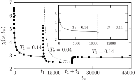
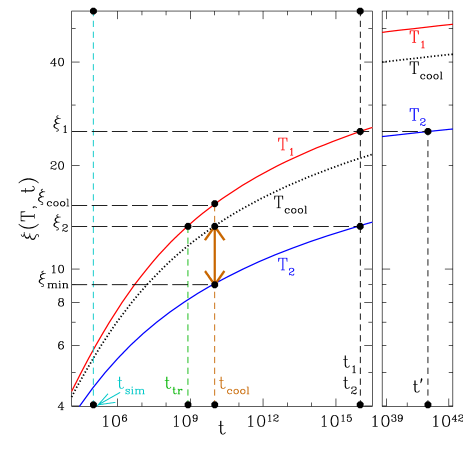
In recent work I we studied the nonequilibrium dynamics of the Heisenberg Edwards-Anderson spin glass model in three dimensions following a sudden quench to its low temperature phase. Here we continue our investigations of the nonequilibrium, low temperature dynamics of this model by analyzing its behavior in more complex protocols, similar to those performed in experiments review1 ; review1_1 ; review3 . More precisely, we consider in detail the effects of a temperature cycle (illustrated in Fig. 1) consisting of the following three steps:

1. Quench the system from $T=\infty$ to a temperature $T_{1}$ at time $t_{\rm w}=0$, and wait a time $t_{1}$.

2. Then change the temperature to a lower value $T_{2}$ and wait a further time $t_{2}$.

3. At total time $t_{\rm w}=t_{1}+t_{2}$ change the temperature back to $T_{1}$.

This temperature cycling protocol has been used extensively to characterize several spin glass systems review1 ; review1_1 ; review3 ; dupuis ; yosh4 ; yosh3 ; bert ; cycle ; physica ; dip ; petra ; kovacs ; india ; matthieu , and these studies motivated similar cycling experiments on many different types of glassy materials struik ; frustre ; leheny1 ; leheny2 ; beta ; KLT ; bellon ; ferro ; ferro2 ; electron .

Numerical studies of temperature shifts and cycles in the Ising version of the model have been reported heiko ; rieger ; yosh2 ; BB1 ; BB2 ; ricci ; ricci2 ; jimenez , and temperature cycles have been discussed theoretically fh ; jorge ; jp ; encorejp ; yosh ; surf ; yosh5_1 ; martin ; yosh5 . However, the Heisenberg spin glass model has been much less studied than its Ising counterpart, even though it is closer to many of the experimentally studied spin glass systems, and only a few aging studies exist I ; II ; ricci2 ; kawa . In particular, extensive studies of temperature cycles have not been reported (see Ref. [ricci2, ] for preliminary results) and we attempt here to fill this gap.

Figure 1: Time evolution of $\chi(\omega,t_{\rm w})$ in a temperature cycle performed with the three-dimensional Heisenberg spin glass for $1/\omega$ = 1078. Aging is observed in the first $t_{1}=11159$ sweeps during which the temperature is at $T_{1}=0.14<T_{c}\simeq 0.16$. The temperature is then quenched to $T_{2}=0.04$ for the next $t_{2}=11159$ sweeps. This causes aging to restart, a rejuvenation effect. The long-dashed line shows the result of a direct quench from $T=\infty$ to $T_{2}$ at time $t_{1}$. The variation of $\chi(\omega,t_{\rm w})$ with $t_{\rm w}$ is much stronger than when the temperature is shifted from $T_{1}$ to $T_{2}$, showing that rejuvenation in the temperature shift is only partial. At $t_{\rm w}=t_{1}+t_{2}$ the temperature is shifted back to its initial value, and the data seems to be simply a continuation of that for $t_{\rm w}<t_{1}$. This memory effect is illustrated more clearly in the inset where the intermediate time spent at $T_{2}=0.04$ has been removed.

The Heisenberg spin glass model that we study has the Hamiltonian

$$H=-\sum_{\langle i,j\rangle}J_{ij}{\bf S}_{i}\cdot{\bf S}_{j},$$ (1)

where the sum is over nearest neighbors of a cubic lattice of linear size $L=60$ with periodic boundary conditions, the ${\bf S}_{i}$ are three-component vectors of unit length and coupling constants are drawn from a symmetric Gaussian distribution of standard deviation unity. We refer to our previous paper I for the technical details concerning our simulations. When performing temperature cycles a large number of parameters can be varied, implying a larger numerical effort than was needed in the simple aging studies of Ref. [I, ].

The basic quantity we measure is the two-time autocorrelation function of the spins, $C(t_{\rm w},t_{\rm w}+\tau)$, defined by

$$C(t_{\rm w},t_{\rm w}+\tau)=\frac{1}{L^{3}}\sum_{i}\langle{\bf S}_{i}(t_{\rm w})\cdot{\bf S}_{i}(t_{\rm w}+\tau)\rangle,$$ (2)

where the brackets indicate an average over both thermal histories and disorder. To compare with experiment we often plot instead

$$\chi(\omega,t_{\rm w})\equiv\frac{1-C(t_{\rm w},t_{\rm w}+\omega^{-1})}{T},$$ (3)

since this is expected to have similar behavior to the ac magnetic susceptibility at frequency $\omega$.

A representative sample of our results for a temperature cycle is shown in Fig. 1. For $t_{\rm w}<t_{1}$ this is just a ‘simple aging’ experiment corresponding to quenching the system infinitely fast from an infinite to a low temperature, $T_{1}=0.14<T_{c}\simeq 0.16$. Physical quantities then slowly relax towards equilibrium, which is known as aging. We have characterized this behavior in detail in Ref. [I, ].

For $t_{1}<t_{\rm w}<t_{1}+t_{2}$, during which the temperature is $T_{2}=0.04<T_{1}$, the signal just after the shift is not a simple continuation of the decay at the previous temperature. The system has apparently forgotten it is already ‘old’ and it seems therefore ‘rejuvenated’ by the temperature change. In experiments performed on Heisenberg spin glasses, when $T_{1}-T_{2}$ is sufficiently large, the signal obtained after the shift can be exactly superposed on the one obtained after a direct quench from $T=\infty$ to $T=T_{2}$, implying that the system behaves as if it had fully forgotten the time spent at temperature $T_{1}$. We will call this situation ‘full rejuvenation’. However, rejuvenation is not full in our simulations because the change in $\chi(\omega,t_{\rm w})$ with time during the part of the temperature cycle at $T_{2}$ is less than the change found in a direct quench to $T_{2}$, which is shown by the long-dashed line in Fig. 1. Since we do not observe full rejuvenation we will need to ask whether the observed behavior is rejuvenation at all or whether it can be fully explained in terms of the cumulative aging scenario, discussed below in Sec. II. We will also investigate the possible origins of this significant difference between numerical and experimental results, and will discuss in particular the role of finite cooling rates in experiments in Secs. III.3 and V.3.

Finally, in the third part of the experiment, $t_{\rm w}>t_{1}+t_{2}$, the relaxation proceeds, after a short transient, as if the second step had not occurred. The system has kept a ‘memory’ of the first aging step despite the strong restart observed in the second part of the protocol. In the inset of Fig. 1, we show that the third part of the experiment appears to be the simple continuation of the first part, as if the second step had not taken place, which we call a ‘perfect memory effect’. This figure is not entirely convincing, though, because the signal is nearly flat and small deviations from perfect memory could be invisible on that scale. That memory is indeed close to perfect, at least for large temperature shifts, will be more quantitatively demonstrated in Sec. IV.

In the rest of this work, we analyze in more detail the rejuvenation and memory effects seen in Fig. 1. Section II gives some theoretical background on the cumulative aging scenario, according to which the effects seen are simply due to changes in the rate of growth of correlations with temperature. Our data on rejuvenation and memory are described in Secs. III and IV respectively. We discuss our results in Sec. V, and give a final summary in Sec. VI.

II Cumulative Aging

An important theoretical concept in understanding non-equilibrium data for spin glasses is that of a dynamical correlation length, $\xi(T,t)$, which describes the spatial extent of spin correlations after aging a time $t$ at temperature $T$. In the cumulative aging scenario, it is proposed that the observed phenomena can be understood solely in terms of the time and temperature dependences of $\xi(T,t)$. We now discuss the predictions of cumulative aging, first for the step down in temperature from $T_{1}$ to $T_{2}$ which can lead to rejuvenation, and then for the subsequent step back up to $T_{1}$ which can lead to memory.

II.1 Cumulative aging and rejuvenation

If the correlation length grows to a value $\xi(T_{1},t_{1})$ by waiting a time $t_{1}$ at $T_{1}$, then one would have to wait a longer time, $t_{\rm eff}^{\rm cum}$, at the lower temperature $T_{2}$ to get the same correlation length, where this ‘effective age’ in the cumulative aging scenario is given by

$$\xi(T_{1},t_{1})=\xi(T_{2},t_{\rm eff}^{\rm cum}).$$ (4)

If the growth law $\xi(T,t)$ is known accurately, Eq. (4) can be used to determine $t_{\rm eff}^{\rm cum}$ for given values of $T_{1},T_{2}$ and $t_{1}$.

In practice one can try to fit the data for $\chi(\omega,t_{1}+t)$ during the time spent at $T_{2}$ to data for $\chi_{{}_{T_{2}}}(\omega,t_{\rm eff}+t)$, i.e. data in a single quench to $T_{2}$ for some waiting time $t_{\rm eff}+t$ with $t_{\rm eff}$ used as a free fitting parameter. In other words $t_{\rm eff}$ is determined from matching both sides of the following equation,

$$\chi(\omega,t_{1}+t)=\chi_{{}_{T_{2}}}(\omega,t_{\rm eff}+t)\,.$$ (5)

One of the following scenarios might then occur. A first possibility is that

$$t_{\rm eff}=0\,,$$ (6)

which corresponds to full rejuvenation. The time spent at $T_{1}$ is irrelevant for aging at $T_{2}$. This is seen experimentally for large temperature shifts, but not in any of our simulations.

Second, one might find that

$$t_{\rm eff}=t_{\rm eff}^{\rm cum}\,,$$ (7)

where $t_{\rm eff}^{\rm cum}$ is given by Eq. (4). This is the so-called cumulative aging scenario. We shall see in Sec. IV.2 that this case describes our simulations when the temperature difference $T_{1}-T_{2}$ is small, though we show in Sec. III.1 that it does not work when $T_{1}-T_{2}$ is large. However, Eq. (7) does not correspond to rejuvenation. Rather, rejuvenation is defined to be the additional effect beyond Eq. (7), since the latter simply reflects the change in the rate of growth of the correlation length with temperature.

A third possibility is that

$$0<t_{\rm eff}<t_{\rm eff}^{\rm cum}\,.$$ (8)

This is one way in which partial rejuvenation could occur, and is seen in some experiments yosh4 ; yosh3 ; petra at intermediate values of the temperature shift. However our simulations do not fit this scenario. Rather, for large values of $T_{1}-T_{2}$ we will see in Sec. III.1 that our data cannot be collapsed on to data for a direct quench by shifting the time. Hence the effective age $t_{\rm eff}$ cannot be defined in our simulations at large temperature differences, and so our results in this region do not fit any of the above scenarios.

Remark that if $t_{1}$ and $T_{1}-T_{2}$ are sufficiently large, $t_{\rm eff}^{\rm cum}$ will be much larger than $t_{1}$. One can make this statement more quantitative by assuming, as usual, that equilibration proceeds by activation over barriers, where the barrier height $\Delta E$ is some function of the length scale $\xi$. Writing $t=t_{0}\exp(\Delta E(\xi)/T)$, where $t_{0}$ is a microscopic attempt time which we set to 1, Eq. (4) gives

$$T_{1}\ln t_{1}=T_{2}\ln t_{\rm eff}^{\rm cum}\,,$$ (9)

which can be written as

$$\ln\left({t_{\rm eff}^{\rm cum}\over t_{1}}\right)=\left({T_{1}-T_{2}\over T_{2}}\right)\ln t_{1}\,.$$ (10)

Hence if $(T_{1}-T_{2})\ln t_{1}>T_{2}$ we have $t_{\rm eff}^{\rm cum}\gg t_{1}$. As a result, $\chi(\omega,t_{1}+t)$, given by Eq. (5), will vary very little with $t$ unless $t$ greatly exceeds $t_{1}$, which is not the case in the simulations. Although the reasoning leading to Eqs. (9) and (10) is for a particular simple model of the growth of the correlation length, we expect the result $t_{\rm eff}^{\rm cum}\gg t_{1}$ to be more generally correct.

II.2 Cumulative aging and memory

In a similar way we can fit the data for $\chi(\omega,t_{1}+t_{2}+t)$ after the step back up to $T_{1}$ to data for $\chi_{{}_{T_{1}}}(\omega,t_{1}+t_{\rm eff}+t)$,

$$\chi(t_{1}+t_{2}+t)=\chi_{{}_{T_{1}}}(\omega,t_{1}+t_{\rm eff}+t),$$ (11)

assuming that the two functions of $t$ in this expression can be matched for a particular choice of $t_{\rm eff}$. If memory is perfect then

$$t_{\rm eff}=0\,,$$ (12)

so that the time spent at $T_{2}$ simply plays no role in the subsequent aging at $T_{1}$.

In the cumulative aging scenario $t_{\rm eff}=t_{\rm eff}^{\rm cum}$ where

$$\xi(T_{1},t_{1}+t_{\rm eff}^{\rm cum})=\xi(T_{2},t^{\prime}+t_{2})\,,$$ (13)

in which $t^{\prime}$ is the time the system would have to age at $T_{2}$ to get the correlation length it reached at $T_{1}$ after time $t_{1}$. It is given implicitly by

$$\xi(T_{2},t^{\prime})=\xi(T_{1},t_{1})\,,$$ (14)

as in Eq. (4) above. This is shown graphically for a set of experimental parameters in Fig. 12 below.

It is worth mentioning that at extremely long times or for very large changes in temperature one expects perfect memory even in the cumulative aging scenario. This is because, at long times, growth of $\xi$ with time at the lower temperature $T_{2}$ is much slower than at $T_{1}$, so $t^{\prime}$ is huge, the difference $\xi(T_{2},t^{\prime}+t_{2})-\xi(T_{2},t^{\prime})$ is small, and hence $t_{\rm eff}^{\rm cum}$ is small. As in Sec. II.1, we can make this more quantitative within a barrier activation model for which Eqs. (13) and (14) imply

$$T_{2}\ln(t^{\prime}+t_{2}) = T_{1}\ln(t_{1}+t_{\rm eff}^{\rm cum})\,,$$ (15)

$$T_{2}\ln t^{\prime} = T_{1}\ln t_{1}\,.$$ (16)

We expect perfect memory if

$$t^{\prime}\gg t_{2}\qquad\mbox{(perfect\ memory).}$$ (17)

Since $t_{1}\sim t_{2}$, from Eq. (16) this gives

$${T_{1}-T_{2}\over T_{2}}\gg{1\over\ln t_{1}}\qquad\mbox{(perfect\ memory)}.$$ (18)

Eq. (17) is equivalent to the condition $t_{\rm eff}^{\rm cum}\ll t_{2}$ since eliminating of $t^{\prime}$ from Eqs. (15) and (16), gives

$${t_{\rm eff}^{\rm cum}\over t_{2}}={T_{2}\over T_{1}}\exp\left[-\left({T_{1}-T_{2}\over T_{2}}\right)\ln t_{1}\right]\,,$$ (19)

assuming $t_{\rm eff}^{\rm cum}\ll t_{1}$. Hence, if Eq. (18) is satisfied, one has perfect memory in the cumulative aging scenario. This conclusion should again be more general than the particular barrier activation model we used.

III Rejuvenation

Now we discuss in detail our results for the behavior following the temperature drop to $T_{2}$ and their interpretation.

III.1 Do we really observe rejuvenation?

Figure 2: The behavior of $\chi(\omega,t_{1}+t)$ during the time $t$ spent at temperature $T_{2}=0.04$ for different values of the time, $t_{1}$, waited at $T_{1}=0.14$. We fix $1/\omega=1078$. For $t_{1}=0$, the system undergoes a direct quench to $T=T_{2}$, while for $t_{1}\to\infty$, the system has time to equilibrate at $T_{1}$. The restart of aging (rejuvenation) is reduced when $t_{1}$ increases from 0, but remains non-zero even when $t_{1}\to\infty$.

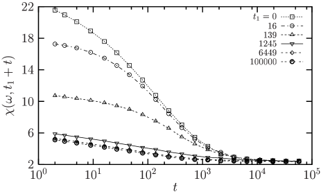
It is clear from Fig. 1 that aging is strongly restarted when temperature changes from $T_{1}=0.14$ to $T_{2}=0.04$, but that, unlike in experiments, the effect is weaker than when the system is directly quenched to $T_{2}$. In Fig. 2 we show the systematic trend in the data when we vary the time $t_{1}$ spent at the upper temperature $T_{1}$. Two important pieces of information can be deduced from Fig. 2.

• The case of $t_{1}=0$ corresponds to a direct quench from $T=\infty$ to $T=T_{2}$. We see from Fig. 2 that the signal obtained after waiting for a finite value of $t_{1}$ at $T=T_{1}$ is different from the signal obtained in a direct quench and differs more as $t_{1}$ is increased. In ‘full rejuvenation’, as seen in experiments, the data after waiting a time $t_{1}$ is the same as in a direct quench. We were not able to vary parameters of temperature cycles in such a way that full rejuvenation is observed in our simulations.

• When $t_{1}$ increases, the signal saturates to a limiting behavior. This is actually the region in which the intermediate part of Fig. 1 was obtained, since $t_{1}$ is quite large there. This saturation implies that even if we were able to equilibrate the system at temperature $T_{1}$, it would undergo aging when further quenched to $T_{2}$. This is very different from the behavior of a pure ferromagnet, for instance, which would reequilibrate on a microscopic timescale upon a similar temperature change within its ferromagnetic phase.

Figure 3: The full lines show data for the two-time spin autocorrelation function $C(t_{1}+t,t_{1}+t+\tau)$ as a function of the time difference $\tau$. The time spent at $T_{1}=0.14$ is $t_{1}=10^{5}$ and the different curves are for different values of $t$, the time waited at $T_{2}=0.04$, increasing from $t=2$ (the lowest) to $t=57797$ in a logarithmic progression. This data shows that aging is restarted in a temperature shift. The dashed lines are the autocorrelation function measured in a direct quench to $T_{2}=0.04$ and waiting times $t=416$, 3728 and 19307 (from left to right). A comparison shows that the shape of the data found in reducing the temperature from $T_{1}$ to $T_{2}$ is different from that in the direct quench to $T_{2}$.

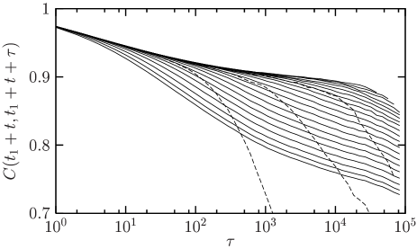
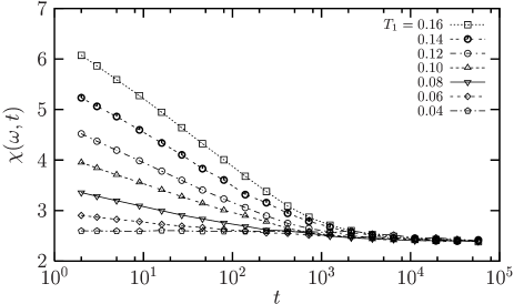
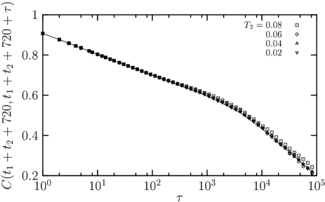
We have therefore seen that rejuvenation is not full. We will now argue that it is not null either and that there is an additional signal beyond that expected in the cumulative aging scenario discussed in Sec. II. To do so it is useful to look at the dependence of $\chi(\omega,t_{1}+t)$ on frequency, or equivalently the dependence of the two-time autocorrelation function on the time difference $\tau$. The solid lines in Fig. 3 show data for this quantity. The system has spent a large time $t_{1}=10^{5}$ at $T=T_{1}=0.14$, sufficiently large that the data in Fig. 3 has become independent of $t_{1}$. The different curves are for different values of $t$, the time waited at $T_{2}=0.04$, increasing from $t=2$ to $57797$ in a logarithmic progression. The curves do not superpose and the behavior observed in Fig. 3 is qualitatively similar to that obtained in simple aging experiments where samples undergo a rapid quench to the spin glass phase. There is a first, fast stationary decay of the autocorrelation functions followed by a second, much slower, age-dependent decay. However, there is a quantitative difference since the precise shape of the data is actually not the same as in a direct quench to $T_{2}$. The difference can be appreciated in Fig. 3 by comparing the solid with the dashed lines, which are for a direct quench with various waiting times. In the direct quench, the correlation function decays faster at long time differences.

For the temperature shift to $T_{2}$ in Fig. 1, we have seen in Fig. 3 that the shape of the extra signal due to this shift is different from the result of a direct quench to $T_{2}$. We also need to ask whether the magnitude of the extra signal is greater than that expected in the cumulative aging scenario discussed in Sec. II.

In Fig. 1, the time $t_{1}=11159$ is large, since the data in Fig. 2 has saturated for this value of $t_{1}$, and the temperature shift $T_{1}-T_{2}$ is large. Hence, as discussed in Sec. II.1, the effective age in the cumulative aging scenario is enormous, and the time dependence of $\chi$ should be tiny in this scenario. This is clearly not the case for the data in Fig. 1. We conclude that for large temperature shifts there is genuine rejuvenation; the cumulative aging scenario does not work. In addition, the fact that the data of Fig. 3 is independent of $t_{1}$, at large $t_{1}$, for all $\tau\equiv\omega^{-1}$, implies that the above conclusion on the existence of rejuvenation holds for any frequency $\omega$ accessible in our simulations.

Figure 4: Top: Changing the second temperature. The protocol is $T=\infty\to T_{1}=0.14$ at time 0. Temperature is kept constant for $t_{1}=11159$ sweeps after which it is shifted to various $T_{2}\leq 0.14$. Bottom: Changing the first temperature. The protocol and notations are as above but with a fixed $T_{2}=0.04$ and different $T_{1}\geq T_{2}$ In both figures the additional amplitude of the aging signal increases with $T_{1}-T_{2}$. While cumulative aging works for small values of $T_{1}-T_{2}$, see Sec. IV, there is a genuine additional rejuvenation signal at large temperature differences.

We note that the use of a different ‘clock’ to determine effective ages could lead to the wrong impression that we observe full (or close to full) rejuvenation yosh3 ; BB2 ; dlogS . If one follows a common experimental procedure and defines $t_{\rm eff}$ as the location of a peak in the logarithmic derivative of the two-time autocorrelation function, $S(t,t+\tau)=\partial C(t,t+\tau)/\partial\log\tau$, one obtains a very small effective age from the data of Fig. 3 and then conclude that rejuvenation is almost full. We know, however, for example by comparing the shapes of the solid and dashed curves in Fig. 3, that this is not the case. Hence $S(t,t+\tau)$ can not be used to quantify rejuvenation in numerical simulations of temperature shifts. This remark was already made for the Ising spin glass in Ref. [BB2, ], although in a less detailed way.

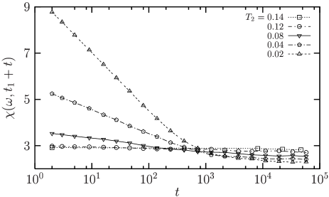
Data for a range of temperature shifts is presented in Fig. 4. We see that the amplitude of the restart of aging is strongly dependent on the amplitude of the temperature shift. The case where $T_{2}=T_{1}$ has no restart of aging and corresponds to a simple quench to $T_{2}$ (with the plot starting at waiting time $t_{1}$). For $T_{2}<T_{1}$ there is an additional decay of $\chi(\omega,t)$ due to the temperature shift. We shall see in Sec. IV.2 that this effect is describable by cumulative aging for small temperature shifts, unlike the situation for large temperature shifts discussed earlier in this section.

As a final comment, we note that the restart of aging observed in the second part of the cycle shown in Fig. 1 is not an artifact produced by our choice of $\chi(\omega,t)$ as a physical observable, as suggested in Refs. [ricci2, ; jimenez, ]. It is certainly true that the susceptibility, defined by Eq. (3) and the correlation function are not related by a fluctuation-dissipation relation since the system is not in equilibrium, and so rejuvenation effects might appear to be stronger using one or the other observable. However, Fig. 3 leaves us with no doubt concerning the fact that aging is restarted in a shift.

III.2 Is temperature chaos relevant?

In this subsection we discuss our results about rejuvenation effects from a theoretical point of view. As already mentioned, the growth of correlations with time is characterized by a dynamical correlation length $\xi(T,t)$. Lengthscales that are active at $T_{1}$ in a given time window $t$, $\xi_{1}\equiv\xi(T_{1},t)$, are typically larger than the ones active at $T_{2}<T_{1}$ in the same time window, $\xi_{2}\equiv\xi(T_{2},t)<\xi_{1}$. Although $\xi(T,t)$ is only a gradual function of $T$ at fixed time $t$, $\xi$ grows very slowly (presumably logarithmically) with $t$ and so it can take an astronomical amount of time to relax excitations of size $\xi_{1}$ at the lower temperature $T_{2}$. Roughly speaking, changing the temperature gives only a modest change in length scales but a huge change in time scales. For practical purposes, excitations of size $\xi_{1}$ are frozen at $T_{2}$ and dynamics at $T_{2}$ is due to fluctuations at the smaller length scale $\xi_{2}$, which had easily reached quasi-equilibrium at temperature $T_{1}$. Rejuvenation therefore means that equilibrium states at $T_{1}$ and $T_{2}$ are significantly ‘different’ on length scales of the order of $\xi_{2}$. What ‘different’ really means will be the subject of this subsection.

Theoretically two explicit examples of this difference have been discussed in the literature:

1. Temperature chaos in the scaling picture of spin glasses fh ; bm1 ; timo ; hajime ; kr .

2. Temperature dependence of the exponent of the power-law decay of spatial correlations in the two-dimensional non-disordered XY model surf .

In the temperature chaos scenario, spin orientations are spatially uncorrelated beyond an overlap length, $\ell_{o}(T_{1}-T_{2})$, which diverges when $T_{1}-T_{2}\to 0$ but is small at large temperature differences, $\ell_{o}\sim|T_{1}-T_{2}|^{-1/\zeta}$, where $\zeta$ is an exponent quantifying chaos. Chaos can therefore naturally explain full rejuvenation if $\ell_{o}<\xi_{2}$ because equilibrium states at the two temperatures are uncorrelated at the important length scale of $\xi_{2}$. As a consequence, aging at $T_{1}$ is unable to bring the system closer to equilibrium at $T_{2}$. In the opposite situation, $\ell_{o}>\xi_{2}$, called ‘weak chaos’, a smaller but non-zero rejuvenation signal should be observed yosh3 , since there are some rare regions of space, occurring with probability $(\xi_{2}/\ell_{o})^{\zeta}$, which are affected by the temperature change.

In the two-dimensional non-disordered XY model below its Kosterlitz-Thouless transition temperature $T_{\rm KT}$, equilibrium spin correlations decay with a power of the distance $r$, $C(\mathbf{r})\sim r^{-\eta(T)}$ where the exponent $\eta(T)$ depends continuously on $T$. This is because there is a line of critical points for $0<T\leq T_{\rm KT}$. Hence, when temperature is changed from $T_{1}$ to $T_{2}$ all length scales have to readjust to the new critical point mauro , whatever the time spent at $T_{1}$. Interestingly this produces a rejuvenation signal which is not full but becomes gradually larger when $T_{1}-T_{2}$ is increased surf .

We now investigate which of these two scenarios corresponds most closely to our simulations. In Ref. [I, ] we showed that spatial spin glass correlations at short distances, $r<\xi(T,t)$, are well-described by algebraic decays with a temperature dependent exponent, $C_{4}(\mathbf{r},t)\sim r^{-\alpha(T)}$ (where $C_{4}$ is defined in Eq. (20) below), just as in the two-dimensional XY model. Moreover, the rejuvenation effect we observe in the present study has the same characteristics as the one found in the XY model, since it is never full but becomes gradually larger when $T_{1}-T_{2}$ is increased. As for the Ising spin glass model BB1 this shows that the rejuvenation signal observed in simulations is largely due the temperature dependence of spatial correlations via the exponent $\alpha(T)$.

It remains to ask, though, whether there are additional rejuvenation effects observed in our simulations due to temperature chaos. In Refs. [BB1, ; BB2, ], it was argued that the answer for three and four dimensional Ising spin glasses is ‘no’. The reason is that chaotic effects with temperature are very hard to detect presumably because the overlap length is never small in Ising systems timo ; hajime . However, equilibrium calculations for vector spins suggest that overlap lengths should be smaller in the Heisenberg case kr , while dynamic length scales are larger than in the Ising model I . Hence it appears potentially easier to detect chaotic temperature effects in Heisenberg systems than in Ising systems II , so this possibility needs to be investigated.

To do so we follow Ref. [BB1, ] and consider a two-site, two-replica correlation function,

$$C_{4}(\mathbf{r},t)={1\over L^{3}}\sum_{i}\langle\mathbf{S}_{i}^{a}(t)\cdot\mathbf{S}_{i+\mathbf{r}}^{a}(t)\ \mathbf{S}_{i}^{b}(t)\cdot\mathbf{S}_{i+\mathbf{r}}^{b}(t)\rangle$$ (20)

where the two replicas $a$ and $b$ have the same interactions but age independently at different temperatures, $T^{a}$ and $T^{b}$, with $\Delta T\equiv T^{a}-T^{b}$. If $\ell_{o}(\Delta T)<\xi(T^{a},t)$ then the overlap between the spin configurations in the two replicas becomes small in a simulation on timescale $t$.

Figure 5: Spatial correlations between two replicas, $a$ and $b$, at equal temperatures $T_{1}=0.14$ (“$T_{1}$”) and $T_{2}=0.04$ (“$T_{2}$”), or different temperatures (“MIXT”). The curve noted “$\sqrt{T_{1}T_{2}}$” is the square root of the product of the data at $T_{1}$ and $T_{2}$ and coincides with the “MIXT” points, as expected in the absence of chaos.

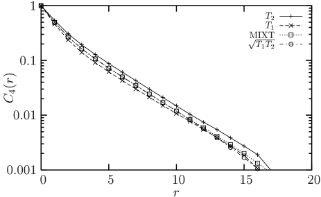
In Fig. 5 we show our results for the Heisenberg model with the same two temperatures $T_{1}=0.14$ and $T_{2}=0.04$ used in our previous cycles. Data is presented for the two-replica correlators in three different cases.

• $T^{a}=T^{b}=T_{1}$, and $t_{\rm w}^{a}=t_{\rm w}^{b}=3728=t_{1}$, noted “$T_{1}$”.

• $T^{a}=T^{b}=T_{2}$, and $t_{\rm w}^{a}=t_{\rm w}^{b}=57797=t_{2}$, noted “$T_{2}$”.

• $T^{a}=T_{1}$, $T^{b}=T_{2}$, $t_{\rm w}^{a}=3728$, and $t_{\rm w}^{b}=57797$, noted “MIXT”.

The simulation times have been chosen so that $\xi(T_{1},t_{1})\simeq\xi(T_{2},t_{2})$. This equality can be seen in Fig. 5 because the correlation functions “$T_{1}$” and “$T_{2}$” are parallel in this log-lin representation at large $r$. By contrast these curves have a different slope at small $r$ because short distance behavior is characterized by the temperature dependent exponent $\alpha(T)$ discussed above.

Since the temperatures $T_{1}$ and $T_{2}$ are very different, we need to take into account the overall increase of spin glass order as the temperature is lowered yosh5_1 . We therefore also plot $\sqrt{C_{4}(r,T_{1},t_{1})C_{4}(r,T_{2},t_{2})}$, which is called “$\sqrt{T_{1}T_{2}}$” in Fig. 5. We find that “MIXT” and “$\sqrt{T_{1}T_{2}}$” are equal within our numerical precision, the result expected in the absence of chaos. We conclude that even weak chaotic effects are not detectable in our numerical simulations despite large temperature jumps, $\Delta T/T_{c}\sim 0.625$, and large dynamic lengthscales, see the range for $r$ in Fig. 5. The dynamic rejuvenation effects we observe can therefore be attributed entirely to the temperature dependence of the exponent $\alpha(T)$ describing the power law decay of spatial correlations at distances less than $\xi(T,t)$.

Of course temperature chaos could still exist at larger length scales. Although the timescales of experiments (relative to the microscopic time) are much longer than in simulations, the difference in length scales is not so pronounced, as we shall emphasize in Sec. V. Hence we feel it is unlikely that strong temperature chaos occurs in experiment either. Unfortunately, this is difficult to check since direct probes of length scales related to chaos effects are not experimentally feasible. As discussed in detail in Sec. V.3, the experimental observation of full rejuvenation does not in itself prove that a strongly chaotic situation is reached in experiments.

III.3 What is a direct quench in experiments?

To our knowledge, full rejuvenation has never been found in numerical studies even in large temperature shifts, in contrast to experiments which do find full rejuvenation. One difference in procedures is that temperature changes in simulations are instantaneous, whereas they can only take place at a finite rate in experiments. We therefore need to study whether correlations built up during gradual cooling are relevant to the subsequent dynamics. If chaos were important in the simulations, the answer would presumably be no, since growth of correlations with time has to restart from scratch at each temperature. However, as we showed in Sec. III.2, no chaos effects are seen in our simulations. Hence we need to consider the effects of gradual changes in temperature, to see whether these modified protocols improve agreement with experiment.

Figure 6: Effect of a non infinite initial temperature in a quench. The system is first quenched from $T=\infty$ to various temperatures, $T_{i}>T_{c}\simeq 0.16$. Temperature is kept constant at $T_{i}$ during $10^{4}$ time steps after which it is quenched to the final temperature $T_{1}=0.04$ at time $t_{\rm w}=0$.

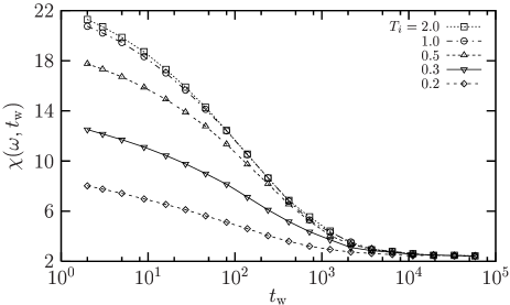
Firstly, rather than quenching from $T=\infty$ to $T_{1}$, we consider the effect of taking a finite initial temperature, $T_{c}<T_{i}<\infty$. This protocol allows us to investigate the effect of building spatial correlations at high temperatures on the aging dynamics at lower temperature. Our results for various $T_{i}$ are presented in Fig. 6 where we have adopted the following procedure. The temperature is quenched from $T=\infty$ to $T_{i}$ where it is kept constant for $10^{4}$ sweeps after which the temperature is instantaneously quenched to the final temperature $T_{1}=0.04$.

For initial temperatures larger than $T_{i}\simeq 2.0\simeq 12.5T_{c}$ the aging observed at $T_{1}=0.04$ is similar to the one observed in a quench from $T_{i}=\infty$. However, as soon as $T_{i}<2.0$ aging is affected. In particular the total amplitude of the relaxation,

$$\Delta\chi(\omega)=\chi(\omega,t=0)-\chi(\omega,t=\infty),$$ (21)

is greatly reduced when $T_{i}$ decreases. We then use Eq. (21) to compare the aging dynamics in various protocols. From Fig. 2 we find that the ratio of the amplitude of relaxation in a truly direct quench to the amplitude in a $0.14\to 0.04$ shift is about 5 while full rejuvenation would imply that this ratio is 1. If, however, one compares the $0.14\to 0.04$ shift to a direct quench from a finite temperature, say from $T_{i}=0.3\simeq 1.9T_{c}$, to $T=0.04$, this ratio becomes $\simeq 2.8$, i.e. closer to the full rejuvenation result. We conclude that spending some time at high temperatures makes the rejuvenation signal closer to what is observed experimentally, though we still do not see full rejuvenation.

In real experiments, not only is the initial temperature finite, as above, but also the cooling from $T_{i}$ to $T_{1}$ is not instantaneous. Therefore not only does the system build correlations at high temperature $T_{i}$, but it also has some dynamics at all temperatures intermediate between $T_{i}$ and $T_{1}$. This is likely to influence even more the aging dynamics at the final temperature.

To investigate this point we have performed simulations of temperature cycles using finite cooling rates. We repeated the temperature cycles of Sec. I using a realistic protocol. The system is first quenched from $T=\infty$ to $T_{i}=2.0$ where it is kept constant during $10^{4}$ sweeps. Then the temperature is decreased at a finite cooling rate, $R$, so that the time evolution of the temperature is of the form $T(t)=T_{i}-Rt$. The cooling is stopped at $T_{1}=0.14$ for a time $t_{1}$, after which the temperature is decreased to $T_{2}=0.04$ at the same cooling rate $R$. We simulated cycles with two different cooling rates, $R_{1}=0.002$ and $R_{2}=0.0005=R_{1}/4$ (cooling rates are expressed in units of $J/t_{0}$ where $J=1$ is the variance of the distribution of coupling constants in Eq. (1) and $t_{0}=1$ is the Monte Carlo time unit). These values were chosen to give cooling times comparable to $1/\omega$, as in experiments india . We find that a finite cooling rate has two effects:

1. All the amplitudes of relaxation are reduced. This is a somewhat natural observation.

2. A less trivial result is that ratio of amplitudes between a direct quench to $T_{2}$ and a shift through $T_{1}$ are again reduced from their $R=\infty$ values. When $1/\omega=1078$, we find that these ratio are 5, 3.8, and 3 for $R=\infty$, $R_{1}$ and $R_{2}$, respectively.

These results again indicate that the finite cooling rates used in experiments, make the observed rejuvenation effects closer to that in experiments, though we are still far from full rejuvenation. In fact, we shall argue in Sec. V.3 that full rejuvenation is expected in experiments because of the much larger range of timescales that are probed there than in the simulations.

Figure 7: Subaging behavior found at $T=0.12$ when the initial temperature is $T_{i}=0.3$ and the cooling rate infinite. The horizontal axis is $u(t_{\rm w},t)=[(t+t_{\rm w})^{1-\mu}-t_{\rm w}^{1-\mu}]/(1-\mu)$ which reduces to $t/t_{\rm w}$ when $\mu=1$, and the vertical axis involves a factor $g(t)$ to account for quasi-equilibrium short-time behavior, see Ref. [I, ] for details. The parameter $\mu$ is adjusted to get the best data collapse for different values of $t_{\rm w}$. The case $\mu<1$, as found here, corresponds to subaging. The case, $\mu=1$, which we find when the initial temperature is $T=\infty$, corresponds to simple aging.

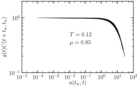
We have shown that a non ideal quench very strongly affects aging behavior. In fact we find that all scaling behaviors reported in Ref. [I, ] for simple aging experiments are affected. This is a likely explanation of the ‘sub-aging’ behavior systematically found in experiments review1 ; india while simulations indicate instead ‘super-aging’ behavior I ; BB1 . As a single example we show in Fig. 7 the effect of a non-infinite initial temperature, $T_{i}=0.3$, on the aging at temperature $T=0.12$. The cooling rate is infinite. When $T_{i}=\infty$ a simple scaling of correlation functions is observed at this temperature I , $C(t_{\rm w},t+t_{\rm w})\sim g^{-1}(t){\cal C}(t/t_{\rm w})$, where $g(t)$ accounts for the short-time quasi-equilibrium behavior. Instead, when $T_{i}=0.3$, we find that a more complicated, sub-aging scaling form is needed, as shown in Fig. 7. We have systematically found sub-aging behavior in non-ideal quenches. Given that experimental cooling times are always extremely large when compared to microscopic timescales it is not surprising that this effect persists experimentally india , unless specific but empirically determined protocols are used cool . Cooling rate effects also imply that aging dynamics probed (a) numerically, and (b) experimentally in ‘direct quenches’, are fundamentally different, which prevents a quantitative comparison of their scaling behavior.

IV Memory

Memory effects are simpler to understand than rejuvenation effects. They directly result from the strong influence of temperature on the timescales needed to equilibrate fluctuations on a given length scale. Dynamics at different temperatures but in similar time windows probe different length scales review3 ; BB1 ; fh ; jp ; encorejp ; yosh5 . In this section we quantify these effects.

IV.1 Is there perfect memory for large shifts?

Figure 8: Time decay of the autocorrelation function $C(t_{1}+t_{2}+720,t_{1}+t_{2}+720+\tau)$ in the third step of temperature cycles with perfect memory. The protocol is as in Fig. 1, i.e. $T_{1}=0.14,T_{2}=0.04,t_{1}=t_{2}=11159$. The waiting time $t_{\rm w}=t_{1}+t_{2}+720$ corresponds roughly to the end of the transient seen in Fig. 1. The full line is the autocorrelation measured in a direct quench to $T_{1}=0.14$ after waiting $t_{1}=11159$, i.e.  $C_{T_{1}}(t_{1},t_{1}+\tau)$. If memory is perfect, the data from the cycle agrees with that from the direct quench. Small deviations from perfect memory are visible at $T_{2}=0.08$, but absent for lower $T_{2}$ for which ‘memory’s perfect’.

In the inset of Fig. 1 we have shown that the aging in the third step of the temperature cycle appears to be, after a short transient, the perfect continuation of the first step. However, this data is not completely convincing because $\chi(\omega,t_{\rm w})$ decreases very slowly on the timescale of the simulation. It is better to study the full frequency dependence, or, equivalently, the time dependence of the spin autocorrelation function BB1 .

In Fig. 8 we show that the memory effect observed in Sec. I is indeed convincing, or, in an allusion to Billy Wilder, that ‘memory’s perfect’ www . The decay of the autocorrelation function in the third stage of the cycle for large $T_{1}-T_{2}$ is indeed the same, within our numerical accuracy, as the one obtained if the second stage of the experiment is dropped out. As in experiments, we conclude that despite the strong rejuvenation effect observed in the second stage at temperature $T_{2}$, the correlations built in the first stage at temperature $T_{1}$ have been perfectly preserved and can be retrieved when temperature is shifted back to its initial value.

IV.2 Is there memory for small shifts?

In the previous subsection we showed that memory is essentially perfect for large temperature shifts. We now discuss what happens for smaller values of the temperature shift where we will see that cumulative aging becomes a good approximation. To compare with the cumulative aging scenario we extract an effective age $t_{\rm eff}$ by fitting the data for $\chi(\omega,t_{1}+t_{2}+t)$ to Eq. (11). Ideally one can find a $t_{\rm eff}$ value so that this data is equal to $\chi_{{}_{T_{1}}}(\omega,t_{1}+t_{\rm eff}+t)$ for all $t$. For technical reasons it is difficult to measure the effective age when times get large because the change in $\chi$ becomes too small. Hence we will extract $t_{\rm eff}$ using a protocol with $t_{1}=0$, i.e. a sudden quench to $T=T_{2}$ followed by an upward shift to $T=T_{1}$ at time $t_{2}$. This modified protocol does not correspond to the cycle discussed in Sec. I but is used here as a convenient mean to measure effective aging times. Also we will actually do the fit to the time dependent correlation function in Eq. (3). This is, of course, equivalent to fitting data for $\chi$.

Figure 9: Influence of the aging at low temperature $T_{2}<0.04$ on the subsequent aging at $T_{1}=0.04$. The system is quenched directly from $T=\infty$ to $T_{2}$ (so $t_{1}=0$), where it is kept during $t_{2}=11159$ time steps, after which the temperature is shifted up to $T_{1}=0.04$. Autocorrelation functions in these shifts are shown with symbols. They are compared to the ones, shown with full lines, measured in a direct quench to $T_{1}=0.04$ and different waiting times $t_{\rm w}=2700$, 4500, 7000 and 9500 (from left to right), chosen to match the temperature shift data. The matching is seen to work well.

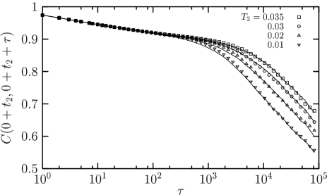
Figure 9 shows some data for this protocol as a function of $\tau=\omega^{-1}$ with $T_{1}=0.04$, $t_{1}=t=0$, and $t_{2}=11159$. Just after the shift up to $T_{1}$ we record the time decay of the spin autocorrelation functions. By definition, when $T_{2}=T_{1}$ the autocorrelation function follows the curve obtained in a direct quench to $T_{1}=0.04$ after $t_{\rm w}=11159$. However, when $T_{2}<T_{1}$ the time decay of the autocorrelation function after the shift becomes faster, but an effective age, $t_{\rm eff}<t_{\rm w}$, can still be defined, since the solid lines in Fig. 9, which are from direct quenches, go through the points, which are from the temperature shift protocol. In other words, matching the correlation functions as a function of $\tau=\omega^{-1}$ to the expression analogous to Eq. (11) with $t_{1}=t=0$ works well. We see from Fig. 9 that $t_{\rm eff}$ progressively decreases when $T_{2}$ decreases, as expected in the cumulative aging scenario of Sec. II. Physically this means that aging at low temperature is less effective at building spatial correlations, or, in other words, that the growth of the dynamic correlation length is slower at lower temperature.

We have repeated this matching procedure for many different shifts, changing $t_{2}$ from 2154 to $2\times 10^{5}$ time steps, the final temperature from $T_{1}=0.4$ to $T_{1}=0.12$, and the amplitudes of the shift, $\Delta T=T_{1}-T_{2}$, from $\Delta T=0.01$ to $\Delta T=0.05$. The results are presented in Figs. 10 and 11 which also contain similar data for the Ising spin glass that are discussed below in Sec. IV.3.

Table 1: Evaluation of the cumulative aging hypothesis in small temperature shifts.

$T_{2}$	$T_{1}$	$t_{2}$	$t_{\rm eff}$	$t_{\rm eff}^{\rm cum}$	$t_{\rm eff}/t_{\rm eff}^{\rm cum}$
0.02	0.04	11159	4500	4200	1.07
0.04	0.08	11159	3000	4200	0.71
0.10	0.12	11159	8000	5500	1.45
0.08	0.12	11159	4700	3800	1.24
0.04	0.08	2154	1350	1300	1.04
0.04	0.08	57797	7500	11000	0.68
0.10	0.12	57797	29000	15000	1.93
0.08	0.12	57797	13000	11500	1.13
0.14	0.12	11159	22500	22000	1.02

We now compare our results for $t_{\rm eff}$ to the prediction of the cumulative aging scenario

$$\xi(T_{1},t_{\rm eff}^{\rm cum})=\xi(T_{2},t_{2})\,,$$ (22)

which is just Eq. (13) with $t_{1}=t^{\prime}=0$. For each of the parameters $T_{1},T_{2}$ and $t_{2}$ corresponding to the points for the Heisenberg model in Fig. 10, we determined $t_{\rm eff}^{\rm cum}$ using Eq. (22) and data for $\xi(T,t)$ in Ref. [I, ]. The ratios of $t_{\rm eff}^{\rm cum}$ to $t_{\rm eff}$ determined from fits like those in Fig. 9 are presented in Table 1. We see that the ratio roughly takes values in the range $[\frac{1}{2},2]$, with no obvious systematic behavior. That the ratio is not perfectly 1 is hardly surprising given that one has to make use twice of imperfect numerical data to estimate $t_{\rm eff}^{\rm cum}$ from Eq. (22). We conclude, contrary to the preliminary investigations of Ref. [ricci2, ] that the cumulative aging hypothesis, Eq. (22), is a good interpretation of the behavior of the Heisenberg spin glass in temperature shifts of small amplitude. Quite importantly, these results validate the assumption of cumulative aging used in Refs. [dupuis, ; bert, ; encorejp, ], where experimental data plotted as in our Figs. 10 and 11 is one of the ingredients used to reconstruct growth laws for $\xi(T,t)$.

Figure 10: The effective age $t_{\rm eff}$ in a shift experiment for different values of $T_{1}$ at fixed $t_{2}$. The system is quenched at $T_{2}=T_{1}-\Delta T$ where it ages during a time $t_{2}=11159$ after which the temperature is shifted up to various temperatures $T_{1}$. Open symbols are for the Heisenberg spin glass, filled symbols for the Ising spin glass. The solid line marked “activation” is the prediction from cumulative aging assuming barrier activation, Eq. (23). The line marked “modified activation” is also for the cumulative aging scenario but assuming different form for $\xi(T,t)$, namely $\xi(T,t)\sim t^{1/z(T)}$ with $z(T)=(T_{0}/T)^{0.85}$, which fits growth laws for the Ising spin glass.

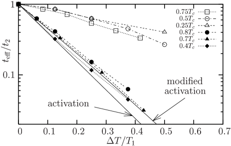
Alternatively, rather than estimate $\xi(T,t)$ from the numerical data of Ref. [I, ], one can assume an analytical form for the growth law, for example the barrier activation model used to obtain Eqs. (9), (15) and (16). This predicts

$$\ln\left({t_{\rm eff}^{\rm cum}\over t_{2}}\right)=-\frac{\Delta T}{T_{1}}\ln t_{2}\,,$$ (23)

which is equivalent to Eq. (9) with the roles of $T_{1}$ and $T_{2}$ interchanged. It corresponds to the straight solid line marked “activation” in Figs. 10 and 11. We find that for all temperatures the measured $t_{\rm eff}$ lie significantly above this result. Moreover, the dependence upon the final temperature $T_{1}$ at fixed $t_{2}$ is weak. From the growth laws for $\xi(T,t)$ reported in Ref. [I, ] this result is reasonable, since the dynamic correlation length is very weakly dependent on temperature for times smaller than $t\sim 10^{3}$ and only after that does it enter a regime dominated by thermal activation I . We therefore expect that shifts performed at larger times $t_{2}$ will get closer to the cumulative aging scenario with a barrier activation form for $\xi(T,t)$.

Figure 11: Effective ages in shift experiments for different values of $t_{2}$ at fixed $T_{1}$. The system is quenched at $T_{1}-\Delta T$ where it ages during a time $t_{2}$. The temperature is then shifted up to $T_{1}$. Open symbols are for the Heisenberg spin glass with $T_{1}=0.08\simeq 0.5T_{c}$, filled symbols for the Ising spin glass with $T_{1}=0.7T_{c}$ but the same times $t_{2}$ as the Heisenberg model. The straight line is the prediction of cumulative aging with thermal activation, Eq. (23).

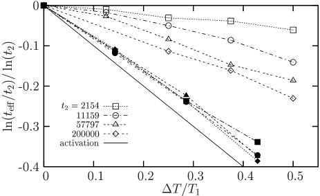
We confirm this expectation in Fig. 11 where we work with a constant final temperature, $T_{1}=0.08\simeq 0.5T_{c}$, but change the duration of the initial period over two orders of magnitude. To compare data with different shifting times, we plot $\ln(t_{\rm eff}/t_{2})/\ln t_{2}$ vs. $\Delta T/T_{1}$ for which cumulative aging with thermal activation, Eq. (23), predicts a linear relation of slope $-1$, independent of $t_{2}$. Upon increasing $t_{2}$ we find that the data get closer to this prediction, but still lie systematically above it. Similar results are found for $T_{1}=0.12\simeq 0.75T_{c}$. As a rough estimate, if the evolution of these curves persists at much larger times it would require about 4 more orders of magnitude, i.e. $t_{2}/t_{0}\sim 10^{9}$, to get curves that eventually lie on or below the thermally activated estimate. This is not inconsistent with the experimental finding that these curves lie below the Arrhenius line in Heisenberg spin glass samples dupuis ; bert ; india since experiments are performed on timescales that are typically $10^{12}$–$10^{16}$ times larger than microscopic flipping times, see e.g. Fig. 12.

In this section we performed upward temperature shifts of relatively small amplitude. We expect that cumulative aging would also work for small temperature changes in a downward shift, but for technical reasons it is difficult to test extensively this hypothesis directly, because effective ages very quickly become too large to be numerically measurable in downward shifts. We nevertheless add in Table 1 the result for a downward $0.14\to 0.12$ shift from the data displayed in Fig. 4a. For this particular example, cumulative aging works indeed very correctly.

IV.3 Does spin anisotropy play a role?

In this subsection we compare our results for the temperature shifts with similar results obtained in the three-dimensional Ising spin glass, using exactly the same thermal protocols and the same procedure to extract effective ages. To this end we needed to extend significantly the numerical results obtained by one of us and Bouchaud in Ref. [BB1, ] to which we refer for technical details concerning the Ising simulations. These new results for the three dimensional Ising Edwards-Anderson spin glass are reported along the ones for the Heisenberg model in Figs. 10 and 11.

A quantitative comparison between the two sets of data can be performed if one assumes that in both cases, Monte Carlo time units represent the microscopic flipping time which we fix to $t_{0}=1$ in both simulations—a physically reasonable assumption. From the comparison between the two models one can draw two main conclusions.

• Curves for the Ising spin glass lie below the ones of the Heisenberg model for all the shifts we have performed, so $t_{\rm eff}/t_{2}$ is smaller for the Ising case. In other words, the effect of a temperature shift on aging dynamics is stronger for the Ising simulations. However, the opposite behavior is observed in experiments which compare strongly anisotropic (Ising) samples with isotropic (Heisenberg) samples bert .

• Changing the duration of the shift over two orders of magnitude has a strong effect on the Heisenberg spin glass, as described in Sec. IV.2 above, but very little or no effect in the Ising case, see Fig. 11. To our knowledge there are no systematic experimental investigations concerning this point but if this trend persists to much larger timescales, it could lead to a situation where Heisenberg data lies below the “activation” curve while Ising data lies above it, as is found experimentally bert .

The Ising data agrees better with the barrier activation form for $\xi(T,t)$ in the cumulative aging picture than does the Heisenberg data. Although we use the terminology “barrier activation” the same result, Eq. (23), applies if the barrier height only depends logarithmically on length scale, in which case rieger ; yosh2 ; ricci2 $\xi(T,t)\sim t^{1/z}$ with $z=T_{0}/T$, i.e. $\xi$ grows with a power of $t$. Recently, algebraic laws with $z=(T_{0}/T)^{\gamma}$ with $\gamma\simeq 0.85$ were reported ricci2 . As shown in Fig. 10 the introduction of the adjustable parameter $\gamma$ allows one to understand deviations from simple thermal activation in the Ising spin glass within the cumulative aging hypothesis. Possibly critical fluctuations near $T_{c}$ renormalize the microscopic flipping time dupuis ; yosh4 ; BB1 in such a way that the growth is approximately of this form in numerical time windows. It would be interesting to check if experimental data taken in anisotropic (Ising) samples can be fitted with the same “modified activation” growth law.

V Discussion

V.1 Memory effects

Memory effects stem from thermally activated dynamics which implies that temperature so strongly influences the growth of the dynamic correlation length, $\xi(T,t)$, that aging is much less effective at building spatial correlations at lower temperatures. Therefore lengthscales that are quasi-equilibrated at some temperature $T_{1}$ can effectively be frozen if the temperature is decreased to $T_{2}<T_{1}$. Spatial patterns imprinted in the systems at $T_{1}$ are then naturally retrieved when temperature is shifted back to its original value. From this perspective it is natural that memory effects are found in so many different disordered materials where activated dynamics is ubiquitous I ; review1 ; review1_1 ; review3 ; dupuis ; yosh4 ; yosh3 ; bert ; cycle ; physica ; dip ; petra ; kovacs ; india ; matthieu ; struik ; frustre ; leheny1 ; leheny2 ; beta ; KLT ; bellon ; ferro ; ferro2 ; electron .

In Fig. 12 we show an example of growth laws as extracted from experimental data in Heisenberg samples in Ref. [encorejp, ]. The precise details of the fits which gave these curves will not be relevant here because our main conclusions will be qualitative. We use this graph to discuss a temperature cycle occurring between temperatures $T_{1}=0.825T_{c}$ and $T_{2}=0.7T_{c}$. Withencorejp $T_{c}=16.7\,{\rm K}$, this gives $T_{1}=13.77\,{\rm K}$ and $T_{2}=11.69\,{\rm K}$, so that $\Delta T\simeq 2\,{\rm K}$, as in the original experiment of Ref. [cycle, ].

Figure 12: Solid curves show $\xi(T,t)$ (with $t$ in units of the microscopic time $t_{0}=10^{-12}\,s$) inferred in Ref. [encorejp, ] for a Heisenberg spin glass at temperatures $T_{1}/T_{c}=0.825$, and $T_{2}/T_{c}=0.7$. Note the break in the horizontal scale between the two boxes. We assume waiting times at $T_{1}$ and $T_{2}$ of $t_{1}=t_{2}=10^{4}\,{\rm s}=10^{16}t_{0}$. The length scales equilibrated at $T_{1}$ and $T_{2}$ are $\xi_{1}\equiv\xi(T_{1},t_{1})$ and $\xi_{2}\equiv\xi(T_{2},t_{2})$ (indicated by horizontal long-dashed lines). To reach length scale $\xi_{1}$ at the lower temperature $T_{2}$ one would have to wait a time $t^{\prime}\simeq 10^{41}\,t_{0}\simeq 3\times 10^{21}\,{\rm years}$, given by Eq. (14). This is truly astronomical, so fluctuations between $\xi_{2}$ and $\xi_{1}$ are effectively frozen during the time $t_{2}$ spent at $T_{2}$, which is the origin of the memory effect. When the temperature is raised back to $T_{1}$, see Fig. 1, fluctuations on length scale $\xi_{2}$ have to reequilibrate at $T_{1}$, which takes a “transient” time $t_{\rm tr}\simeq 10^{9}=10^{-3}\,{\rm s}$ (which is very short; another requirement for perfect memory). We also show $t_{\rm cool}$, the time spent ‘close to’ a given temperature during cooling, and indicate, by a dotted line, the growth at $T=T_{\rm cool}=0.795T_{c}$, the temperature at which $\xi(T_{\rm cool},t_{\rm cool})$ is equal to $\xi_{2}$. We also define $\xi_{\rm cool}=\xi(T_{1},t_{\rm cool})$. In cooling to $T=T_{2}$ the system will have correctly equilibrated for temperature $T_{2}$ up to scale $\xi_{\rm min}=\xi(T_{2},t_{\rm cool})$. During subsequent aging for time $t_{2}$ at $T=T_{2}$, fluctuations on scales between $\xi_{\rm min}$ and $\xi_{\rm cool}$ (shown by the thick line with arrows) have to reequilibrate, which gives rise to rejuvenation. The time scale probed in our simulations is of order $t_{\rm sim}\simeq 10^{5}$, which is much smaller than in experiments. However, the difference between the length scales probed in experiment and simulations is much smaller than the difference in timescales.

For concreteness we assume a microscopic time of $t_{0}=10^{-12}\,{\rm s}$ and take $t_{1}=t_{2}=10^{4}\,{\rm s}$ so, in units of the microscopic time, we have $t_{1}=t_{2}=10^{16}$. The correlation lengths $\xi_{1}$ and $\xi_{2}$ reached at $T_{1}$ and $T_{2}$ in a time $t_{1}=t_{2}$ are 25.3 and 13.3 respectively, indicated by dashed horizontal lines. To reach a length scale of $\xi_{1}$ at the lower temperature $T_{2}$ would require an astronomically large time of order $t^{\prime}\simeq 10^{41}\,{\rm t_{0}}=10^{29}\,{\rm s}$, given by Eq. (14), which is indicated in the right hand box of the figure. Also relevant is an estimate of the transient time, $t_{\rm tr}$, required to reequilibrate fluctuations at scale $\xi_{2}$ when the temperature is increased back to $T_{1}$. This is given implicitly by $\xi(T_{1},t_{\rm tr})=\xi_{2}\equiv\xi(T_{2},t_{2})$. From Fig. 12 we see that $t_{\rm tr}$ is of order $1\,{\rm msec}$, hardly detectable if the frequency is of the order of a few Hz. In general, we expect perfect memory if Eq. (17) and the condition

$$t_{\rm tr}\ll t_{2}\qquad\mbox{(needed\ for \ perfect\ memory)},$$ (24)

are both satisfied. Within the barrier activation model and for $t_{1}\sim t_{2}$, Eqs. (24) and (17) are actually equivalent since this model predicts that

$${\ln t_{2}\over\ln t_{\rm tr}}={\ln t^{\prime}\over\ln t_{1}}={T_{1}\over T_{2}}.$$ (25)

Equation (18), which corresponds to Eq. (17) for the barrier activation model, is satisfied for the experimental situation in Fig. 12, so memory should be perfect, as was indeed found cycle . However, Eq. (18) is harder to satisfy in numerical simulations since the timescales are shorter. Hence larger temperature steps have to be chosen in simulations, but, nonetheless, Eq. (18) can then be satisfied. This conclusion holds for both Heisenberg and Ising spin glass models heiko ; yosh2 ; BB1 ; ricci ; ricci2 ; jimenez .

While the details of the numbers in this discussion can be debated, it is surely true in general that changing the temperature in experiments gives a large change in timescales (though not a very large change in length scales), and that perfect memory can be obtained in this situation with moderate to large temperature shifts.

V.2 Physical origin of rejuvenation effects

We have seen in Sec. V.1 that to get memory it is sufficient to have a wide separation of time scales. We now turn to rejuvenation effects which are more difficult to understand since, by itself, Fig. 12 does not explain why aging is strongly restarted when the temperature is shifted from $T_{1}$ to $T_{2}$. The important question is that, since excitations on lengthscales active at $T_{2}$ were fully equilibrated at $T_{1}$ just before the shift, why do they need to reequilibrate at all upon a small temperature change?

In this paper we have been able to answer this question for the Heisenberg spin glass model simulated on timescales up to $10^{5}$. We find that spatial correlations at equilibrium (i.e. at distances less that $\xi(T,t)$) are close to algebraic with a temperature dependent exponent $\alpha(T)$ so that excitations on all lengthscales up to $\xi$ have to readapt at each temperature. This interpretation is very close to the physical interpretation of the behavior of the two-dimensional XY model when temperature is shifted along its critical line surf .

As discussed in Section III.2 we found no trace of chaotic behavior of spatial correlations with temperature, though it is possible that chaotic effects could set in at larger lengthscales. However, in the hypothetical temperature cycle of Fig. 12, which corresponds to experimental parameters, we see that the difference in lengthscales probed by simulations and experiments is not very drastic (a factor of about 3 or 4) so we are tempted to conclude that chaos also does not occur in experiments. Even if it did, chaotic effects would appear in addition to the signal characterized in this paper, so experimental results would present a mixed character, difficult to analyze quantitatively within one scenario or the other.

The situation found here is qualitatively very similar to what is observed numerically in Ising spin glasses in various dimensions heiko ; yosh2 ; BB1 ; BB2 ; ricci . Differences between models arise only at a quantitative level. For instance, in the three dimensional Ising spin glass, the exponent $\alpha$ only depends weakly on temperature taking the value of about $0.5$ throughout the spin glass phase BB1 . Correlations change more significantly in four dimensionsBB1 with $\alpha$ changing from 0.9 and 1.6 between $0.5T_{c}$ and $T_{c}$. As a result, rejuvenation effects are relatively pronounced in four dimensions, while almost absent in three yosh2 ; ricci . By comparison, $\alpha$ in the three dimensional Heisenberg spin glass has an intermediate behavior I since it changes from 0.8 to 1.1 between $0.5T_{c}$ and $T_{c}$. However this relatively small variation is compensated by the fact that dynamic lengthscales for the Heisenberg model are also larger than for the Ising case.

V.3 Experimental observation of full rejuvenation

We have seen in Sec. V.2 that the observation of partial rejuvenation in the simulations for large temperature shifts can be well understood. Here, we give a plausible explanation of the full rejuvenation observed experimentally, an important ingredient being a very large separation of time scales, much larger than is feasible in simulations.

As mentioned in Section III.3, ‘direct’ quenches in experiment are not instantaneous, and incorporating this into the simulations gave results which were somewhat closer to full rejuvenation. Here we develop a phenomenological description of aging which includes a finite cooling rate. An important concept in it is the time spent ‘close to’ a given temperature cooling , where a precise definition of ‘closeness’ will not be needed to illustrate the main points qualitatively, but presumably requires that spatial correlations (on the cooling timescale) do not change ‘much’ while the temperature is ‘close’ to a given value. Let us denote this timescale by $t_{\rm cool}$. As an example, if we assume that a quench takes place in $1\,{\rm s}$, and divide this time into 100 intervals, we have $t_{\rm cool}=0.01\,{\rm s}=10^{10}t_{0}$, as indicated in Fig. 12. This is certainly rough, but we can vary $t_{\rm cool}$ quite substantially without invalidating our main conclusions.

It will be convenient, for the subsequent discussion, to define various length and time scales which arise in quenching down to $T=T_{2}$ at a given rate. Correlations on length scale $r$ will freeze, i.e. drop out of equilibrium, at temperature $T_{\rm f}(r)$ where

$$\xi(T_{\rm f}(r),t_{\rm cool})=r\,.$$ (26)

To determine the extent of rejuvenation in a $T$-shift to $T_{2}$, we need to consider the correlations on length scales up to $\xi_{2}$. The temperature where correlations on this scale fall out of equilibrium is

$$T_{\rm cool}=T_{\rm f}(\xi_{2})\,,$$ (27)

which is $T_{\rm cool}\simeq 0.795T_{c}$ in the example shown in Fig. 12. During the cooling process, when the temperature has reached $T=T_{1}$ the correlation length will be

$$\xi_{\rm cool}\equiv\xi(T_{1},t_{\rm cool})\,$$ (28)

see Fig. 12. When the system has been cooled down to $T=T_{2}$, the system will be equilibrated for this temperature up to scale

$$\xi_{\rm min}=\xi(T_{2},t_{\rm cool}),$$ (29)

which is also shown in Fig. 12.

We are now in a position to compare aging after a ‘direct quench’ to $T_{2}$ with that following a temperature shift from $T_{1}$ to $T_{2}$. Suppose first that $T_{1}>T_{\rm cool}$ (i.e. $\xi_{\rm cool}>\xi_{2}$), which is the situation in Fig. 12. Then the time spent waiting at $T_{1}$ will have no effect on the behavior at $T_{2}$ because this will only change correlations at scales larger than $\xi_{2}$ that are anyway frozen at $T_{2}$. The important correlations are those of scales between $\xi_{\rm min}$ and $\xi_{2}$ and these only freeze out during the subsequent cooling from $T_{\rm cool}$ to $T_{2}$, see Fig. 12. Provided correlations on length scales between $\xi_{\rm min}$ and $\xi_{2}$ depend on temperature (through the temperature dependence of the exponent $\alpha(T)$), these will have to reequilibrate while waiting at $T_{2}$, and so there will be a rejuvenation signal. Furthermore, the signal will be same for the direct quench and the temperature shift from $T_{1}$, i.e. we have full rejuvenation.

On the other hand, if $T_{1}<T_{\rm cool}$ (so $\xi_{\rm cool}<\xi_{2}$) waiting at $T_{1}$ does enhance correlations at scales $\leq\xi_{2}$ (to be precise, at scales between $\xi_{\rm cool}$ and $\xi_{2}$) relative to a direct quench. Hence rejuvenation will only be partial in this case.

Hence we can succintly express the condition for full rejuvenation as

$$\xi_{\rm cool}>\xi_{2}\quad\mbox{(full\ rejuvenation)},$$ (30)

or in other words,

the correlation length developed at $T=T_{1}$ during cooling is greater than the correlation length subsequently developed during waiting at the lower temperature $T=T_{2}$.

To get a rough idea of the numbers implicit in Eq. (30), we take the simple barrier activation model for $\xi(T,t)$ discussed in Sec. II in which $\xi(T,t)$ is assumed to be a function of $T\ln t$. The condition for full rejuvenation, Eq. (30), then becomes

$${T_{1}-T_{2}\over T_{2}}>{\ln(t_{2}/t_{\rm cool})\over\ln t_{\rm cool}}\qquad\mbox{(full\ rejuvenation)}.$$ (31)

The deviations from simple barrier activation used in the plots in Fig. 12 actually allow full rejuvenation when $T_{1}$ is somewhat closer to $T_{2}$ than given by Eq. (31). Since we need $t_{2}\gg t_{\rm cool}$ (otherwise the signal is dominated by initial transients), Eq. (31) implies that $t_{2}$ must be huge.

Given our numerical results I for $\xi(T,t)$, we estimate that $t_{\rm cool}>10^{3}$ is at least necessary to satisfy Eq. (30), implying that the total cooling time is about $10^{5}$, so that aging times should be $t_{1}\sim t_{2}\gg 10^{5}$ which is not presently feasible in simulations. This justifies our inability to reach the full rejuvenation limit in this numerical work, as opposed to experimental investigations. By contrast, perfect memory effects can be obtained in simulations because they do not rely on the existence of finite cooling rates; compare Eqs. (18) and (31).

Figure 13: Effect of a stop during cooling on the zero-field cooled magnetization. The duration of the stop is $t_{\rm stop}=5\times 10^{4}$, and two temperatures $T_{\rm stop}=0.14$ (squares) and $T_{\rm stop}=0.08$ (circles) are used, as shown by vertical arrows. We plot the difference between $M_{\rm stop}$ and $M_{\rm zfc}$, the zero-field cooled magnetizations with and without the stop, respectively. The cooling and heating rates are $R=5\times 10^{-6}$, the magnetic field is $h=0.01$. A dip centered around $T_{\rm stop}$ is observed, but this is broader than in experiments.

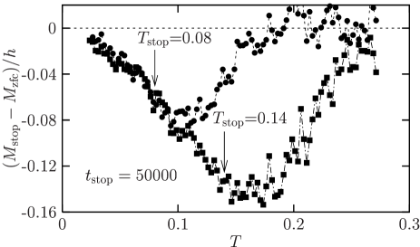
We also suspect that Eq. (31) is necessary to observe the spectacular ‘dip’ in ac susceptibility measurementsdip . The reason a sharp dip has not been seen in simulationsricci is, in our view, because the timescales did not satisfy Eq. (31). In an effort to get closer to Eq. (31), we have reproduced the experimental protocol of Ref. [matthieu, ] where a dip experiment is realized using the magnetization as a physical observable. The system is gradually cooled at rate $R=5\times 10^{-6}$ from high temperature, $T_{i}=0.35$, to very low temperature $T=0.02$. It is then immediately reheated at the same rate $R$ with a small magnetic field, $h=0.01$, which ensures linear response fdt . The zero field cooled magnetization, $M_{\rm zfc}(T)$, is then recorded. We then repeat the same protocol but this time include a stop of duration $t_{\rm stop}$ at temperature $T_{\rm stop}$ during cooling. Upon reheating we now measure $M_{\rm stop}(T)$. The difference $M_{\rm stop}-M_{\rm zfc}$ for $t_{\rm stop}=5\times 10^{4}$ and two different temperatures, $T_{\rm stop}=0.14$ and $T_{\rm stop}=0.08$ is presented in Fig. 13. Curves have the typical shape found in experiments matthieu where the difference is maximal close to $T_{\rm stop}$ and becomes 0 at smaller and larger temperatures. However the dip found here is broader than in experiments. The fact that the curve has a bump at $T_{\rm stop}$ is akin to a memory effect since upon reheating the system remembers it has aged there. The fact that the difference diminishes at $T<T_{\rm stop}$ is a rejuvenation effect, because despite having aged close to $T_{\rm stop}$ the magnetization gets close to the reference curve. A full rejuvenation would imply that the difference really goes to 0. As above, we do find a good amount of memory but only a partial rejuvenation, because the separation of timescales is smaller than in experiments.

Recently, experiments have been carried out on superspin glasses petra , in which the microscopic timescale $t_{0}$ is considerably larger than in standard spin glasses ($t_{0}\simeq 10^{-5}{\rm s}$), and so the timescales probed are closer to those of our simulations than in experiments on standard spin glasses. Interestingly, results of these experiments are quite similar to those of our simulations and, in particular, rejuvenation is only partial even when temperature steps are quite substantial. In our view, the claim made in Ref. [petra, ] that rejuvenation is “absent” is merely a matter of definition, and we prefer to say that rejuvenation exists but is not full. Lack of full rejuvenation observed in superspin glasses is consistent with our discussion if the spread of timescales is not large enough for Eq. (30) or (31) to be satisfied. Implicit in Ref. [petra, ] is the idea that full rejuvenation necessarily implies strong temperature chaos. However, we have argued here that full rejuvenation does not require temperature chaos; just a large separation of time scales and a temperature shift which is not too small.

VI Summary

We have numerically studied memory and rejuvenation effects in the three dimensional Heisenberg Edwards-Anderson spin glass. The main difference between experiments and simulations is that the simulations have a much less pronounced separation of timescales. As a result, memory effects in temperature cycles can only be observed numerically for larger temperature shifts than in experiments.

Similarly, we find that the timescale gap between experiments and simulations also produces a qualitative difference when Ising and Heisenberg models are compared. In our numerical time window, the effect of a temperature shift on aging dynamics is stronger for Ising systems than for Heisenberg systems, see Fig. 10 and Sec. IV.3, since the dynamic correlation length varies more strongly with $T$ in the Ising case. However, in experiments, the effect is the opposite bert ; india . The numerical data shift, but only slowly, towards experimental observations when larger timescales are simulated, see Fig. 11.

In addition to memory effects, we also observe partial rejuvenation for large temperature shifts. However, we find no sign of temperature chaos even for much larger temperature shifts than in experiment. The main difference between the results of simulations, including ours, and experiments is that simulations never find full rejuvenation. We have given an explanation of this which does not involve temperature chaos but rather depends on (i) the finite cooling rate in experiments and (ii) the much larger separation of time scales in experiments than in simulations. The finite cooling rate also appears to be the explanation for the ‘sub-aging’ behavior found in experiments.