Also at ]L. D. Landau Institute for Theoretical Physics, Chernogolovka, Russia

Soliton phase near antiferromagnetic quantum critical point in Q1D conductors

Abstract

In frameworks of a nesting model for Q1D organic conductor at the antiferromagnetic (SDW) quantum critical point the first-order transition separates metallic state from the soliton phase having the periodic domain structure. The low temperature phase diagram also displays the 2nd-order transition line between the soliton and the uniformly gapped SDW phases. The results agree with the phase diagram of (TMTSF)₂PF₆ near critical pressure [T. Vuletic et al., Eur. Phys. J. B 25, 319 (2002)]. Detection of the 2nd-order transition line is discussed. We comment on superconductivity at low temperature.

We address the issue of quantum critical point (QCP) for the itinerant antiferromagnetism (AFM) (also known as spin-density wave state (SDW)) in Q1D compounds. As it was pointed out in Hertz , the standard renormalization group (RG) analysis is not applicable for superconductivity QCP and theoretical models for AFM with nesting features because no expansion in a form of a Landau functional is possible near QCP at $T=0$ in these cases. QCP with increase in pressure have been observed for SDW in the Bechgaard salts (TMTSF)₂X (with X=PF₆ Jerome1980 , AsF₆ Brus ) and recently investigated in many details in Vuletic . According to Vuletic , the phase diagram of (TMTSF)₂PF₆ near its critical pressure, $p_{c}\sim 9.4$kbar, indeed, has a rather complicated character. However, the experimental fact that the transition from metallic to SDW state is of the first order suggests that quantum fluctuations do not play decisive role near $p_{c}$, and the overall phase diagram near $p_{c}$ for (TMTSF)₂PF₆ can be understood already on a mean field level.

The most unexpected finding in Vuletic is the discovery of a pressure interval below $p_{c}$, where SDW and metal phases (SDW and superconductivity (SC) at lower $T$) coexist as parallel domains running perpendicular to the chain direction. Such coexistence is difficult to understand for the 1st order transition that takes place at constant pressure Vuletic . In what follows we propose that such domains can be interpreted as formation of a new phase of the soliton walls suggested first theoretically for the Q1D electron spectrum in BGS ; BGL ; GL . Domains inside the SDW interval were also observed in LeeChaikin . We shall see that it is rather natural to expect SC in these domains at lower temperature. In this presentation we restrict ourselves mainly by the effects related to the physics of SDW. Superconductivity appears at lower temperature than the onset of the SDW/metal phase transition, and we only comment on it at the end.

For the SDW description we adopt the standard Q1D model of two open Fermi surface (FS) sheets with the energy spectrum of free electrons in the form:

$$\varepsilon(\bm{p})=\pm v_{F}(p_{x}\mp p_{F})+t_{\perp}(\bm{p}_{\perp}),$$ (1)

with dispersion in the direction perpendicular to the chains

$$t_{\perp}(\bm{p}_{\perp})=t_{b}(\bm{p}_{\perp})+t^{\prime}_{b}(\bm{p}_{\perp}).$$ (2)

The condition

$$\left<t_{b}(\bm{p}_{\perp})\right>_{\bm{p}_{\perp}}=\left<t^{\prime}_{b}(\bm{p}_{\perp})\right>_{\bm{p}_{\perp}}=0$$ (3)

is assumed to conserve the number of electrons. The angular brackets mean averaging over $p_{\perp}$:

$$<..>_{\bm{p}_{\perp}}\equiv\int(..)(b/2\pi)dp_{\perp}.$$

The component $t_{b}(\bm{p}_{\perp})$ possesses the so-called ”nesting” feature (at $t^{\prime}_{b}\equiv 0$) favoring formation of the SDW gap along the two sheets of the Fermi surface. For that one needs

$$\varepsilon(\bm{p}+\bm{Q})=-\varepsilon(\bm{p}).$$ (4)

”Antinesting” term, $t^{\prime}_{b}(\bm{p}_{\perp})$, destroys the perfect nesting condition (4). Increase of $t^{\prime}_{b}$ simulates increase in applied pressure. At large enough $t^{\prime}_{b}$ SDW disappears.

The model assumes a bare e-e interaction of the form

$$u(\bm{Q})\bm{\sigma_{1}}\bm{\sigma_{2}},$$ (5)

where $u(\bm{Q})$ has a maximum at some $\bm{Q}_{0}$. Interaction (5) is renormalized after summing up the ladder diagrams:

$$U(\bm{Q})=\frac{u(\bm{Q})}{1+u(\bm{Q})\Pi(\bm{Q},\omega_{0})}.$$ (6)

The polarization operator

$$\Pi(\bm{Q},\omega)=T\sum_{\omega_{n}}\int\frac{d^{2}\bm{p}}{(2\pi)^{2}}G(\bm{p},\omega_{n})G(\bm{p}-\bm{Q},\omega_{n}-\omega)$$ (7)

is proportional to the staggered susceptibility. Its value is large near a ”nesting” vector $\bm{Q}_{0}$. Most often this vector is chosen as

$$\bm{Q}_{0}=(\pm 2p_{F},\pi/b,\pi/c),$$ (8)

although the majority of the results below do not change, at least qualitatively, at different optimal ”nesting” wave vectors $\bm{Q}_{0}$. For brevity, in (2) we shall leave out the dependence on the third direction along the $c$-axis Com2 .

When the denominator in (6) becomes zero, the metal phase is absolutely unstable with respect to a SDW(CDW) nucleation. The instability line $T_{c}(t_{b}^{\prime},\bm{Q})$ is given by a well-known equation:

$$\ln\left(\frac{T_{c0}}{T_{c}}\right)=\mbox{Re}\left<\Psi\left(\frac{1}{2}+\frac{iW(\bm{Q},p_{\perp})}{4\pi T_{c}}\right)\right>_{p_{\perp}}-\Psi\left(\frac{1}{2}\right),$$ (9)

where $T_{c0}$ is the temperature of the SDW onset at $t_{b}^{\prime}=0$ and $W(\bm{Q},p_{\perp})=\hbar v_{F}(Q_{x}-2k_{F})+t_{\perp}(p_{y})+t_{\perp}(p_{y}-Q_{y})$. Eq. (9) has been analyzed by many authors (see, e.g. BGL ; HasFuk ; Montambaux ; Jafarey ). At zero temperature Eq. (9) writes down as BGL

$$\left<\ln\left(\pi T_{c0}/\gamma W(\bm{Q},p_{\perp})\right)\right>_{p_{\perp}}=0,$$ (10)

where $\gamma\approx 1.781$ is the Euler constant.

With increasing pressure the value of $t_{b}^{\prime}$ increases, and at some critical pressure $p_{c}$ the SDW ordering may disappear even at zero temperature. This point could be considered as QCP. However, one sees that the application of renormalization group (RG) analysis Hertz to QCP in Q1D case would meet difficulties because an analytic expansion of Eq. (10) at small $\bm{q}\equiv\bm{Q}-\bm{Q}_{0}$ does not exist due to the condition (3).

The integral (10) is convergent at any finite $\bm{Q}$, and one can find critical $t_{b}^{\prime}$ for the general form of $t_{\perp}(p_{\perp})$. It does not necessarily occur at $\bm{Q}=\bm{Q}_{0}$, but at some $\bm{Q}^{*}\equiv\bm{Q}_{0}+\bm{q}^{*}$ Comment1 . Transition into such a new SDW phase with ”shifted” wave vector (SDW₂ phase) should be of the second order, and, hence contradicts to the observed 1st-order character of the transition between SDW and the metal phase in Vuletic .

It is known that for strictly 1D models of CDW (or SDW) the character of excitations is different from the ordinary one. Instead of electron-hole pairs with excitation energy $\approx 2\Delta$, the propagating excitations are solitons (or soliton ”kinks”) that cost a lower energy and come about together with the nonlinear reconstruction of the underlying gaped ground state Su ; Braz . (TMTSF)₂PF₆ has a quarter filled band ($2k_{F}=\pi/2a$). Unlike the Peierls state in polyacetylene, (CH)_x , commensurability effects play here no essential role JeromeReview , so that only the neutral spin $1/2$ solitons exist Braz . Below we merely borrow the results from the extended literature on solitons in a 1D chain (for a review and references, see BrazKirovaReview ). Although this literature is devoted to the physics of CDW state, all the results can be transferred to the SDW case, practically, without changes.

The energy cost for one soliton ”kink” on a single 1D chain is

$$E_{s}=(2/\pi)\Delta_{0}.$$ (11)

For chain packed in a crystal a tunneling, $t_{\perp}(p_{\perp})$, arise between the chains. Therefore, the solitons form extended states by creating a band in the transverse direction. Instead of independent kinks on different chains, one arrives at a soliton wall BGS with neutral solitons occupying two spin states with $t_{\perp}(p_{\perp})<0$ in the band . The energy cost $A(t_{\perp})$ of the wall referred to one chain decreases,

$$A(t_{\perp})=(2/\pi)\Delta_{0}-2\int_{t_{\perp}\leq 0}t_{\perp}(p_{\perp})bdp_{\perp}/2\pi,$$ (12)

and may even become negative. In other words, the spontaneous formation of soliton wall may be favorable at large enough $t_{\perp}$.

Eq.(12) presents our key idea for interpreting the phase diagram of (TMTSF)₂PF₆ Vuletic : with the pressure increase the system first reaches a critical pressure, $p_{c1}$, at which $A(t_{\perp})=0$, and smoothly enters into a new phase – the soliton phase (SP). At some higher pressure ($p_{c}$) the first-order transition between SP and metallic phase takes place.

To describe the sequence of such transitions, one needs expressions for the energy of SP. The problem was solved in BGL for the CDW ordering and for ”direct” nesting vector $\bm{Q}_{0}=(\pm 2k_{F},0)$. Change from CDW to SDW needs no explanation. Without staying on the proof, we remark that the gauge transformation of the wave functions, as in BGL , removes the large ”nesting” term $t_{b}(p_{\perp})$ from all expressions below. As the result, it is only the ”antinesting” term $t^{\prime}_{b}(p_{\perp})$ that enters Eq. (12): $t_{\perp}(p_{\perp})\rightarrow t^{\prime}_{b}(p_{\perp})$.

We now write down the expression for the linear energy density $W_{SP}$ of the soliton phase BGL in the limit of large distance between the walls($T=0$):

$$W_{SP}=-\frac{\Delta_{0}^{2}}{2\pi\hbar v_{F}}+nA(t_{b}^{{}^{\prime}})+nE_{-}^{2}B,$$ (13)

where $n$ is the walls’ linear density, and the $E_{-}^{2}$ term in (13) correspond to the exponentially decaying interaction between the walls. Indeed, in this limit of large distances between walls, $n$ from BGL

$$n=\frac{E_{+}/\hbar v_{F}}{K\left(\sqrt{1-E_{-}^{2}/E_{+}^{2}}\right)}\approx\frac{\Delta_{0}/\hbar v_{F}}{\ln\left(4\Delta_{0}/E_{-}\right)},$$ (14)

where $E_{+}\approx\Delta_{0}$ at $n\to 0$ and $K(r)$ is the complete elliptic integral of the 1st kind. From (14)

$$E_{-}\approx 4\Delta_{0}\exp(-\Delta_{0}/n\hbar v_{F}).$$

$A(t_{b}^{{}^{\prime}})$ is given by Eq. (12) with $t_{\perp}(p_{\perp})=t^{{}^{\prime}}_{b}(p_{\perp})$, and

$$B(t_{\perp})=\frac{1}{2\pi\Delta_{0}}-\frac{b}{|dt^{{}^{\prime}}_{b}/dp_{\perp}|_{0}},$$ (15)

where $|dt^{{}^{\prime}}_{b}/dp_{\perp}|_{0}$ is the value of the transverse velocity at the four point where $t^{{}^{\prime}}_{b}(p_{\perp})=0$. At $B>0$ crossing the point $A(t^{{}^{\prime}}_{b})=0$ corresponds to the second-order transition from the ”homogeneous” SDW to the soliton walls lattice state. Negative $B<0$ would mean an abrupt first-order phase transition BGL . All the results (12-15) are for $T=0$.

We now return to Eq. (9). As the absolute instability line, at higher temperature it defines the 2nd-order transition line between the metal and SDW(CDW) phase. At lower temperature for most $t_{b}^{{}^{\prime}}(p_{\perp})$ models it corresponds to some ”shifted” $\bm{Q}^{*}$. As it was mentioned above, experimentally Vuletic , the metal-to-SDW transition at lower temperature is of the 1st-order. At these temperatures the line defined by Eq. (9) has only the meaning of a ”supercooling” line.

Theoretically, the positions of critical points $p_{c}$ and $p_{c1}$ depend essentially on a particular form of $t^{\prime}_{b}(p_{\perp})$. The function $t^{\prime}_{b}(p_{\perp})$ in (TMTSF)₂PF₆ is unknown. Therefore, for qualitative analysis we will apply the expressions (14),(15) also in the regime of dense soliton phase. We compare two examples: first, the oversimplified model, in which $t^{\prime}_{b}(p_{\perp})$ has the periodic step-like shape:

$$t^{{}^{\prime}}_{b}(p_{\perp})=\biggl{\{}\begin{array}[]{c}2t^{{}^{\prime}}_{b},\ 0<p_{\perp}<\pi/b\\ -2t^{{}^{\prime}}_{b},\ \pi/b<p_{\perp}<2\pi/b\;,\end{array}$$ (16)

and the second one with the tight-binding dispersion of the form

$$t^{\prime}_{b}(p_{\perp})=2t_{b}^{\prime}\cos(2p_{\perp}b)$$ (17)

We calculated the energy of the soliton phase for both dispersion functions. At the calculation the optimal value of $E_{-}$ (or $n$) must be found to minimize the energy (13) of the soliton phase. For the first dispersion (16) the domain wall energy $A(t^{\prime}_{b})$ becomes negative at $t^{\prime}_{b}\geq t_{c1}\approx 0.32\Delta_{0}$. This point corresponds to the 2nd-order transition from ”homogeneous” SDW phase into the soliton phase. Then we compared the soliton phase energy $W_{SP}$ with the energy of metal phase

$$W_{n}=-(1/\pi\hbar v_{F})\left<[t^{\prime}_{b}(p_{\perp})]^{2}\right>_{p_{\perp}}$$ (18)

and found the point $t_{c}\approx 0.54\Delta_{0}$ where these energies become equal to each other. This point corresponds to the first-order phase transition from SP to the normal-metal phase. We see that the interval $t_{c}-t_{c1}\approx 0.4t_{c}$ of the existence of SP for this particular model is rather large. One can show that for the model described by Eqs. (12)-(15) the function (16) correspond to the largest possible interval of SP.

For the second dispersion relation (17) the similar calculation gives equal values for $t_{c}$ and $t_{c1}$: $t_{c}=t_{c1}=\Delta_{0}/2$, i.e. in this case an interval for soliton phase is absent. This once more shows the high sensitivity of the SDW phase diagram to the particular form of $t^{{}^{\prime}}_{b}(p_{\perp})$.

In experiment Vuletic the difference $t_{c}-t_{c1}\approx 0.1t_{c}$ is intermediate between the cases of Eq. (16) and Eq. (17), but closer to the second case of tight-binding dispersion relation (17) than to the step-like dispersion (16). The ratio $(t_{c}-t_{c1})/t_{c}\approx 0.1$ observed in experiment Vuletic can be easily fitted by an appropriate choice of the model function $t^{{}^{\prime}}_{b}(p_{\perp})$ (for example, by adding a fourth harmonic to the tight-binding dispersion (17).

In Fig. 1 we show schematically the SDW phase diagram near QCP. The slope of the second-order transition line near $T=0$ comes about because at $T\neq 0$ the second term in $A(t_{\perp})$ decreases to account for thermal excitations inside the domain wall from the occupied part of band $t^{{}^{\prime}}_{b}(p_{\perp})<0$. The temperature slope, of course, again depends on the $t^{{}^{\prime}}_{b}(p_{\perp})$-dependence.

In Vuletic the phase diagram of (TMTSF)₂PF₆ has been studied through the resistance measurements along the chain direction. The 1st-order character of the transition between metal and SDW states follows from hysteretic effects, while the appearance of domains was derived from the changes in resistivity behavior near $p_{c}$. We suggest that the line of the 2nd-order transition between the insulating ”homogeneous” and soliton-wall phases could be detected by measuring a sharp anisotropy of conductivity near this transition GL . Indeed, according to GL , at low $n$ (large distance between the domain walls) conductivity along the chain direction remains very low because of exponentially small overlap between the electron wave functions inside each wall. As for transverse conductivity, it would increase linearly with $n$.

One also sees that the value of $t^{\prime}_{b}$ itself is not the only parameter that may determine the dependence on $t^{\prime}_{b}$ (pressure). Indeed, the expression for $B(t_{\perp})$ (15) essentially depend on $|dt^{{}^{\prime}}_{b}/dp_{\perp}|_{0}$ as well. The $B$-term is not analytic at $t^{\prime}_{b}\to 0$; change in its sign will immediately change the whole physics BGL .

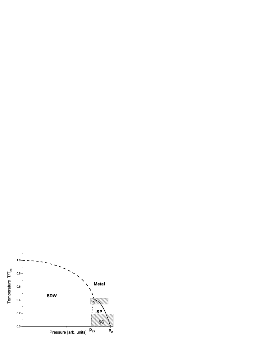
Figure 1: A schematic view of the SDW phase diagram. The solid line signify the first-order transition between the metal and soliton phases. The dot line stands for the second-order transition between uniformly gapped SDW phase and the SP. The dash line represents the line of absolute instability of metal phase toward the formation of SDW. At higher temperatures this line represents the second-order transition line between the SDW and metal phases. At lower temperature (dash-dot line) it has only the meaning of supercooling line. The lower filled bars shows the region where superconductivity appears. We do not calculate the superconducting critical temperature. The upper filled bar shows the high-temperature region of soliton phase where substantial quantitative deviations from formulas (12)-(15) may start due to the thermal excitations in the SDW and soliton phases. Detailed shape of all lines is sensitive to the choice of the ”antinesting” term $t^{{}^{\prime}}_{b}(p_{\perp})$ (see text).

In Fig. 1 the superconductivity, seen experimentally in Vuletic near $p_{c}$ and in the metallic phase at lower temperatures ($T_{c}\sim 1K$), is not shown in order not to overcrowd the phase diagram. Meanwhile, appearance of superconductivity is inevitable in frameworks of nesting mean-field models. Indeed, the logarithmic singularity that enters the expression for SDW polarization operator (7), would appear also for the Cooper channel BGD . At higher temperature the SDW phase prevails because the bare interaction (5) was chosen to be larger for the transverse nesting component $\bm{Q}_{\perp}$. However, with increase of ”antinesting” term $t^{\prime}_{b}$ (pressure) the SDW transition becomes suppressed and SC which is not sensitive at all to any of the $t^{\prime}_{b}$-terms, finally becomes more favorable. To some surprise, $T_{SC}$ for the SC transition is experimentally not sensitive to the formation of the SP. We explain this fact qualitatively by assuming that the SC coherence length, $\xi_{0}\sim\hbar v_{F}/T_{SC}$, is considerably larger than the expected periodicity for the SP of the order of $\hbar v_{F}/\Delta_{0}\sim\hbar v_{F}/T_{0}$ resulting in considerable Josephson coupling between the soliton walls. However, the problem needs some further analysis.

To summarize, we have shown that in the vicinity of QCP in Q1D materials, such as the Bechgaard salts, one meets with a new soliton wall phase. As the pressure increases from $p=0$, one first crosses the line $p_{c1}$ of the second-order transition and enters into the periodic soliton structure with a characteristic pressure-dependent periodicity of the order of $\hbar v_{F}/\Delta_{0}\sim 10^{3}$Å. At higher pressure, $p_{c}$, by the first-order phase transition the system goes over into metallic state. Details of the phase diagram strongly depend on material parameters, in particular on the form of the ”antinesting” tunneling in the electron dispersion. Coexistence of SDW and superconductivity inside soliton walls has not been investigated. Qualitatively one would expect the survival of superconductivity in the ”metallic sheets” (domain walls) perpendicular to the chain direction GL .

The authors acknowledge useful discussions with S.A. Brazovskii. The work was supported by NHMFL through the NSF Cooperative agreement No. DMR-0084173 and the State of Florida, and (PG) in part, by DOE Grant DE-FG03-03NA00066.

References

- (1) T. Vuletic, P. Auban-Senzier, C. Pasquier et al., Eur. Phys. J. B 25, 319 (2002).
- (2) J.A. Hertz and M.A. Klenin, Phys. Rev. B 10, 1084 (1974).
- (3) D. Jerome et al., J. de Phys. Lett.44, L-49 (1980).
- (4) R.Brusetti,M. Ribault, D. Jerome and K. Bechgaard, J. Phys. France 43, 801 (1982).
- (5) S.A. Brazovskii, L.P. Gor’kov, J.R. Schrieffer, Physica Scripta 25, 423 (1982).
- (6) S.A. Brazovskii, L.P. Gor’kov, A.G. Lebed’, Sov. Phys. JETP 56, 683 (1982) [Zh. Eksp. Teor. Fiz. 83, 1198 (1982)].
- (7) L.P. Gor’kov, A. G. Lebed, J. Phys. Colloq. Suppl. 44, C3-1531 (1983).
- (8) I.J. Lee, P.M. Chaikin and M.J. Naughton, Phys. Rev. Lett. 88, 207002 (2002).
- (9) In the most Q1D organic compounds the electron dispersion in -direction is very weak, and its ”antinesting” part (that the only influences the phase diagram) is negligible.
- (10) Y.Hasegawa and H. Fukuyama, J. Phys. Soc. Japan 55, 3978 (1986).
- (11) G. Montambaux, Phys. Rev. B 88, 207002 (2002).
- (12) S. Jafarey, Phys. Rev. B 16, 2584 (1977).
- (13) There exists the extended literature devoted to the two SDW states in the Q1D compounds (see, e.g., HasFuk ; Montambaux ). It dates back to the numerical calculations in HasFuk . These calculations contains some wrong results that we correct in a separate publication.
- (14) W.P. Su, J. R. Schrieffer and A. J. Heeger, Phys. Rev. Lett. 42, 1698 (1979); Phys. Rev. B 22, 2099 (1980).
- (15) S.A. Brazovskii, Sov. Phys. JETP 51, 342 (1980).
- (16) D. Jerome, H.J. Schulz, Adv. Phys. 31, 299 (1982).
- (17) S.A. Brazovskii and N.N. Kirova, Sov. Sci. Rev. A Phys., 5, 99 (1984).
- (18) Such a strong interplay between two phases reflects the well-known fact that in the strictly 1D limit the logarithmic singularities appear simultaneously in the Cooper and ”zero-sound” channels. Their separation comes about due to the presence of some 3D features [Yu.A. Bychkov, L.P. Gor’kov, I.E. Dzyaloshinskii, Sov. Phys. JETP 23, 489 (1966)].