Frustration of Decoherence in Open Quantum Systems

Abstract

We study a model of frustration of decoherence in an open quantum system. Contrary to other dissipative ohmic impurity models, such as the Kondo model or the dissipative two-level system, the impurity model discussed here never presents overdamped dynamics even for strong coupling to the environment. We show that this unusual effect has its origins in the quantum mechanical nature of the coupling between the quantum impurity and the environment. We study the problem using analytic and numerical renormalization group methods and obtain expressions for the frequency and temperature dependence of the impurity susceptibility in different regimes.

I introduction

In physics there is a large class of problems that can be described in terms of a single quantum mechanical degree of freedom interacting with an environment. Examples range from magnetic impurities in metals, superconductors, and magnets, macroscopic quantum tunneling in superconducting interference devices (SQUIDS) and molecular magnets mqt , to qubits in quantum computers qc . The common thread between all these problems is the dramatic effect that the dissipation has on the quantum dynamics of the impuritycl . In particular, one of the most important effects of an environment on a quantum system is decoherence, that is, the destruction of quantum mechanical effects. Decoherence is the unavoidable consequence of the fact that no system in nature is really isolated.

Impurity problems can be often reduced to an effective one-dimensional boundary problem that allows the use of powerful non-perturbative theoretical techniques. The Kondo model is probably one of the best known impurity problems and has been studied with a large number of theoretical tools, from the exact solution via Bethe ansatz bethe , numerical renormalization group nrg , to conformal field theory cft . The Kondo problem represents a universality class of open quantum systems where dissipation and decoherence play a fundamental role. In its anisotropic form, the Kondo effect can be mapped via dimensional reduction and abelian bosonization to the ohmic dissipative two-level system (DTLS) problemdtls . The Kondo effect can be thought as a situation where decoherence is extreme, in the sense that the spin is completely screened by the environmental excitations in the formation of the so-called Kondo singlet. Moreover, impurities can be used as probes for the understanding of the environment itself and in some cases can even determine the properties of the environment in a self-consistent manner. This occurs in the case of the dynamical mean-field theories (DMFT) where the solution of a many-body problem reduces to the solution of a self-consistent impurity problem dmft . Furthermore, systems where the competition between different phases of matter lead to the appearance of magnetic inhomogeneities (such as in the case of Griffiths-McCoy singularities in heavy fermion alloys) can many times be reduced to effective impurity problems griffiths .

In this paper we are going to describe a model for open quantum systems that cannot be described within the Kondo universality class. This model describes an effect that we call frustration of decoherence where decoherence is reduced by a pure quantum mechanical effect. It is important, therefore, that one understands the physics behind the standard model of dissipation described by the Kondo or the DTLS and how it relates to the problem of decoherence. Since the connection between the Kondo problem and decoherence is not commonly discussed in the literature we will review some of the key features of the DTLS and its connection with the problem of decoherence.

The DTLS can be described as a single spin half, ${\textbf{S}}=(S_{1},S_{2},S_{3})$, coupled to a set of independent harmonic oscillators via the Hamiltonian (we use units such that $\hbar=1=k_{B}$):

$$H_{\mathtt{DTLS}} = \Delta S_{3}+\frac{i\lambda}{\sqrt{2L}}S_{1}\sum_{k>0}\sqrt{k}(a_{k}-a_{k}^{\dagger})$$ (1)

$$+ \sum_{k}vka_{k}^{\dagger}a_{k},$$

where $\Delta$ is the tunnel splitting between the eigenvalues of $S_{1}$, $\lambda$ is the coupling to an environment of bosons with one-dimensional momentum $k$, and energy dispersion $\omega_{k}=vk$ ($v$ is the velocity of the excitations that we set to unity, $v=1$, from now on) and creation and annihilation operators $a_{k}^{\dagger}$ and $a_{k}$, respectively ($L$ is the linear size of the system). The operators obey canonical commutation relations:

$$[a_{k},a_{k^{\prime}}^{{\dagger}}] = \delta_{k,k^{\prime}}$$

$$\left[S_{i},S_{j}\right] = i\epsilon_{ijk}S_{k}$$ (2)

where $\epsilon_{ijk}$ is the Levi-Civita antisymmetric tensor. In this model one assumes a cut-off energy $\Lambda$, where $\Lambda$ is some non-universal quantity that is associated with microscopic properties of the bath ($\Lambda$ is usually proportional to the inverse of the lattice spacing $a$).

The physics described by Hamiltonian (1) can be summarize as follows. When $\vec{S}$ is decoupled from the environment ($\lambda=0$) one has an isolated spin problem in the presence of a “magnetic field” proportional to $\Delta$. If at certain time $t=0$ the spin is prepared in an eigenstate of $S_{1}$, the “magnetic field” induces transitions between the eigenstates of $S_{1}$ and the expectation value of the operator $S_{1}$, namely, $\langle S_{1}(t)\rangle$, oscillates harmonically with frequency $\Delta$. There is no release mechanism for the energy in the spin. By switching on a small coupling to the bath of oscillators, the harmonic oscillations of $\langle S_{1}(t)\rangle$ become underdamped due to the dissipation. Second order perturbation theory indicates that the behavior of the system depends on a dimensionless coupling $\alpha=\lambda^{2}/8\pi$. For $\alpha<1/2$ there are two main effects saleur : the slow modes of the bath, that cannot follow the motion of the spin, lead to damping and therefore to an exponential decay of $\langle S_{1}(t)\rangle$; the fast modes of the bath, that can follow the motion of the spin, lead to a new renormalized oscillation frequency $\Delta_{R}<\Delta$. For $\alpha>1/2$ there is a crossover to an overdamped regime where oscillations disappear (effectively $\Delta_{R}\to 0$) and only exponential decay occurs. Finally, at $\alpha=1$ there is a true quantum “phase transition”, where the the impurity spin becomes localized in one of the eigenstates of $S_{1}$. In the Kondo language the change from delocalized to localized is equivalent to a Kosterlitz-Thouless transition (KT) between the Kondo problem with ferromagnetic coupling (that has a triplet ground state) and the Kondo problem with antiferromagnetic coupling (with a singlet as ground state).

One of the most illuminating ways to describe the KT transition is via a perturbative renormalization group (RG) calculation in leading order in $\Delta/\Lambda\ll 1$. The RG proceeds in two steps. In the first step one reduces the cut-off energy of the bosonic bath from $\Lambda$ to $\Lambda-d\Lambda$ by tracing out high energy degrees of freedom. In a second step the dimensionless coupling constants $\alpha$ and $h=\Delta/\Lambda$ are rescaled to the new cut-off leading to the RG equationsdtls :

$$\frac{d\alpha}{d\ell} = -h^{2}\alpha\,,$$ (3a)

$$\frac{dh}{d\ell} = (1-\alpha)h\,$$ (3b)

where $d\ell=d\Lambda/\Lambda$. Thus, for $\alpha>1$ the system scales under the RG to weak coupling ($h(\ell)\rightarrow 0$), and at low energies the tunneling splitting $\Delta(\ell)$ scales towards zero leading to localization. Conversely, for $\alpha<1$ the couplings scales towards strong coupling ($h\rightarrow\infty$) indicating that RG breaks down. The renormalization scheme fails at a certain energy scale (that is, the value of $\ell=\ell^{*}$ for which $h(\ell^{*})\approx 1$). This characteristic scale is called the Kondo temperature that can be obtained directly from (3) as: $T_{K}\approx\Lambda(\Delta/\Lambda)^{1/(1-\alpha)}$. In the Kondo problem, for frequencies and temperatures below $T_{K}$ there is no reminiscence of the original impurity spin. This is an extreme example of decoherence.

Although the RG equations clearly captures the asymptotic behavior of the spin dynamics, in order to observe the cross-over from underdamping to overdamping, one has to look at the frequency and temperature dependence of the spin correlation functions. This is even more important in the context of decoherence, since we are interested in measuring observables associated with the local degrees of freedom, not with the environment. In a spin problem, a particular apropos object is the impurity transverse susceptibility that is given by:

$$\chi_{\perp}(\omega) = -i\int_{0}^{\infty}\frac{dt}{2\pi}e^{i\omega t}\langle[S_{1}(t),S_{1}(0)]\rangle\,.$$ (4)

The imaginary part of $\chi(\omega)$, $\chi^{\prime\prime}(\omega)$, is a measure of the amount of energy that is dissipated from the spin into the environment. In the absence of coupling to the environment ($\lambda=0$ in (1)) we have $\chi^{``}(\omega)\propto\delta(\omega-\Delta)$ indicating the spin “oscillates” freely with frequency $\Delta$. When $\lambda>0$ two different effects occur in the frequency behavior of $\chi^{\prime\prime}(\omega)/\omega$: (1) instead of a Dirac delta function one finds a broadened peak and $\chi^{\prime\prime}(\omega)/\omega$ becomes finite at $\omega=0$, indicating that the oscillations become damped; (2) the maxima moves from $\Delta$ to a renormalized value $\Delta_{R}$ due to “dressing” of the spin by fast environmental modes. In the DTLS, the value of $\chi^{``}(\omega)/\omega|_{\omega\to 0}$ and its width $\delta\omega$ are set by the $T_{K}$: $\chi^{``}(\omega)/\omega|_{\omega\to 0}\propto 1/T^{2}_{K}$ and $\delta\omega\propto T_{K}$. In particular, in the overdamped regime ($\alpha>1/2$) the peak in $\chi^{``}(\omega)$ at finite frequency vanishes completely leaving a smooth function centered around $\omega=0$ costi .

In this paper we are going to study a model that can be considered a generalization of the DTLS (1):

$$H = \sum_{k>0}k\left(a_{k}^{\dagger}a_{k}+b_{k}^{\dagger}b_{k}\right)+\Delta S_{3}$$ (5)

$$+ \frac{i}{\sqrt{2L}}\sum_{k>0}\sqrt{k}\left\{\lambda_{1}S_{1}(a_{k}-a_{k}^{\dagger})\right.$$

$$+ \left.\lambda_{2}S_{2}(b_{k}-b_{k}^{\dagger})\right\}$$

where there are two independent dissipative baths labeled by operators $a_{k}$ and $b_{k}$ with couplings $\lambda_{1}$ and $\lambda_{2}$. Notice that (5) reduces to the DTLS, eq. (1), when one of the couplings $\lambda_{1}$ or $\lambda_{2}$ vanishes. At first sight, the only apparent difference between (5) and (1) is the existence of an additional bosonic bath coupled to a third spin component. Thus, naively one would expect an enhancement of decoherence in comparison with the DTLS since more heat baths are present. This naive argument fails to grasp that both baths are “competing” with each other for the “ordering” of the impurity. While the coupling $\lambda_{1}$ “tries” to localize the spin in an eigenstate of $S_{1}$, the coupling $\lambda_{2}$ also “tries” to localize the spin in an eigenstate of $S_{2}$. However, we see from (2) that the operators $S_{1}$ and $S_{2}$ do not commute with each other and therefore one cannot find a common eigenstate for the spin to localize in. This purely quantum mechanical effect leads to a less decoherent environment. We will show that when $\lambda_{1,2}=\lambda$ and $\Delta/\Lambda\ll 1$ the spin dynamics is always in the underdamped regime, regardless of the bare value of the coupling constants. In our previous publication we called this state of affairs the “quantum frustration of decoherence” prl .

The Hamiltonian (5) was originally obtained in the study of an spin $1/2$ impurity embedded in an environment of large spin-S in $d=3$ dimensions prl . The mapping between these two problems is given in appendix A. The magnetic environment has two effects in the dynamics of the impurity. The molecular fields produced by the environmental spins favor the alignment of the impurity spin along the ordering direction giving rise to a “magnetic field” proportional to $\Delta$. The transverse magnetic fluctuations (spin waves) produce quantum fluctuations that tend to misalign the impurity spin leading to couplings proportional to $\lambda_{1,2}$ and therefore to dissipation. In an ordered antiferromagnetic spin environment the low energy, long-wavelength excitations, are two massless Goldstone modes (two transverse magnon excitations) that couple to the two different components of the spin as in (5). The problem of impurities in magnetic media, especially in the paramagnetic phase, has received a lot of attention in the context of quantum phase transitions subir ; vojta . As we are going to show in what follows, the effect of quantum frustration occurs at finite energies or frequencies and therefore before the asymptotic regime is reached (very low frequencies) and the impurity spin fully aligns with the environmental spins. Thus, as in the case of the Kondo problem, quantum frustration is a crossover phenomenon that cannot be obtained in “asymptopia”. We should stress, however, that the phenomenon of quantum frustration is more general than its origin would imply. As in the case of the Kondo effect, it represents a universality class of impurity problems where decoherence is reduced by pure quantum mechanical effects.

As mentioned above, impurity problems can be treated by powerful theoretical techniques when reduced to one-dimensional models with a boundary. It is convenient, therefore, to rewrite (5) in a real space representation:

$$H = \int_{-\infty}^{+\infty}dx\sum_{a=1,2}\left(\partial_{x}\phi_{a}(x)\right)^{2}+\Delta S_{3}$$ (6)

$$- \sqrt{8\pi\alpha_{1}}\partial_{x}\phi_{1}(0)S_{1}-\sqrt{8\pi\alpha_{2}}\partial_{x}\phi_{2}(0)S_{2},$$

where $\phi_{1,2}(x)$ are one dimensional chiral bosonic fields (that is, left movers only) associated with the bosonic modes $a_{k}$ ($b_{k}$) and we have defined $\alpha_{1,2}=\lambda_{1,2}^{2}/8\pi$. We are ultimately interested in the general problem of decoherence described by (5) or (6) and the mechanism of quantum frustration associated with this model.

The paper is organized as follows: we derive the main RG equations in Section II and show that the dissipative model discussed here is always coherent and shows scaling at strong coupling; in Section III we study the impurity susceptibility using numerical renormalization group and analytical RG via the Callan-Symansky equations; Section IV contains a discussion of the problem of frustration of decoherence and also our conclusions. There are various appendices where the details of the calculations have been included.

II renormalization group

Notice that, according to the RG equations (3), the KT transition occurs at a finite value of the coupling constant $\alpha$ and therefore cannot be obtained directly from perturbation theory. Instead, one has to use a rotated basis of states, obtained from a unitary trasnformation, where the problem becomes perturbative. This can be accomplished in our case by defining two unitary transformations:

$$U_{1} = e^{i\frac{\pi}{2}S_{2}}e^{i\sqrt{8\pi\alpha_{1}}\phi_{1}\left(x=0\right)S_{3,}}$$ (7a)

$$U_{2} = e^{i\frac{\pi}{2}S_{1}}e^{i\sqrt{8\pi\alpha_{2}}\phi_{2}\left(x=0\right)S_{3}}\,,$$ (7b)

that rotate the impurity spin around the $S_{3}$ direction by angles that depend on the field configurations and around $S_{2}$ ($S_{1}$) by $\pi/2$. Notice that $U_{1}$ ($U_{2}$) generates a non-perturbative rotation in terms of the coupling $\alpha_{1}$ ($\alpha_{2}$).

Let us consider the problem after rotation by $U_{1}$. By applying $U_{1}$ to the Hamiltonian (6), we obtain

$$U_{1}^{\dagger}HU_{1}=H_{0}+\frac{1}{2}\left(\Delta A_{1}^{+}+i\sqrt{8\pi\alpha_{2}}B_{1}^{+}\right)+\mathtt{h}.\mathtt{c}.$$ (8)

where $H_{0}$ is the free bosonic Hamiltonian (the first term in the left hand side of (6)). We have defined two vertex operators,

$$A_{1}^{\pm} = e^{\mp i\sqrt{8\pi\alpha_{1}}\phi_{1}\left(x=0\right)}S^{\pm},$$ (9a)

$$B_{1}^{\pm} = \partial_{x}\phi_{2}\left(x=0\right)e^{\mp i\sqrt{8\pi\alpha_{1}}\phi_{1}\left(x=0\right)}S^{\pm},$$ (9b)

where $S^{\pm}=S_{1}\pm iS_{2}$ are the standard raising (lowering) operators.

As in the case of a generalized Coulomb gas problem cg ; ayh , the partition function of the problem, $Z$, can be obtained in the basis that diagonalizes $S_{3}$ ($S_{3}|s_{3}\rangle=\pm\frac{1}{2}|s_{3}\rangle$) as

$$Z = \sum_{\left\{S^{z}\right\}}\int D\phi_{1,2}(x,\tau)\,e^{-S_{0}[\phi_{1,2}(x,\tau)]}\,\prod_{j}\frac{\delta\tau}{2}\left[\Delta A_{1}^{m_{j}}\left(\tau_{j}\right)\right.$$ (10)

$$+ \left.im_{j}\sqrt{8\pi\alpha_{2}}B_{1}^{m_{j}}\left(\tau_{j}\right)\right]$$

where $S_{0}$ is the action for the free boson fields, $\delta\tau$ is the time step in the imaginary time direction, and $m_{j}=s_{3}\left(\tau_{j}+\delta\tau\right)-s_{3}\left(\tau_{j}\right)$ is either $+1$ for a kink or $-1$ for an anti-kink at time $\tau_{j}$ of a given spin history in imaginary time. The partition function given in (10) is the starting point of the RG analysis.

We can define the Fourier transforms of the vertex operators, $A_{1}(\omega)=\int d\tau\exp\{i\omega\tau\}A_{1}(\tau)$ and bosonic fields $\phi_{1,2}(k,\omega)=\int dx\int d\tau\phi_{1,2}(x,\tau)\exp\{i(kx-\omega\tau)\}$, and divide the fields into slow modes, say $A_{1,<}(\tau)$, with $(\omega,k)<\Lambda$ and fast modes, say $A_{1,>}(\tau)$ with $(\omega,k)>\Lambda$. We then integrate the fast modes within a shell $\Lambda<\left(k,\omega\right)<\Lambda+d\Lambda$, to obtain the renormalization of the slow fields due to the fast modes. In this procedure the renormalization of the slow modes is given by averages over the fast modes. It is straightforward to show that:

$$\left\langle A_{1}^{\pm}\left(\tau\right)\right\rangle_{>} = A_{1,<}^{\pm}\left(\tau\right)e^{-\alpha_{1}d\ell}$$ (11a)

$$\left\langle B_{1}^{\pm}\left(\tau\right)\right\rangle_{>} = B_{1,<}^{\pm}\left(\tau\right)e^{-\left(1+\alpha_{1}\right)d\ell}$$ (11b)

where, $d\Lambda/\Lambda=d\ell$ and $\langle P\rangle_{>}$ indicates the average of the operator $P$ over the fast modes. Substituting (11) into (10) and rescaling the fields in order to obtain the same partition function with slow modes only, we find that the couplings have to change with $\ell$ according to (see Appendix B):

$$\frac{d\alpha_{2}}{d\ell} = -2\alpha_{1}\alpha_{2}$$ (12a)

$$\frac{dh}{d\ell} = \left(1-\alpha_{1}\right)h\,,$$ (12b)

which define the RG equations for $\alpha_{2}$ and $h$ but not for $\alpha_{1}$. The RG equation for $\alpha_{1}$ is obtained in second order in $h$. In the language defined by Anderson-Yuval-Hamann ayh , it corresponds to the renormalization in $\alpha_{1}$ due to a “close pair” of flip and anti-flip that is removed from a spin history in a particular RG step. One can show that a new operator, which is not present in the original problem is generated under this procedureNovais02 . This operator reads:

$$C\approxeq 1-i\sqrt{2\pi\alpha_{1}}h^{2}\partial_{\tau}\phi_{1}\left(0,\tau\right)S_{3}\left(\tau\right)d\ell\delta\tau.$$ (13)

This term can be reexponentiating into the action, Eq. (10), and then integrated by parts in $\tau$. The final result is equivalent to a redefinition of the vertex operators,

$$A_{1}^{\pm} = e^{\mp i\sqrt{8\pi\alpha_{1}}\left(1-\frac{1}{2}h^{2}d\ell\right)\phi_{1}\left(0\right)}S^{\pm},$$ (14a)

$$B_{1}^{\pm} = \partial_{x}\phi_{2}\left(0\right)e^{\mp i\sqrt{8\pi\alpha_{1}}\left(1-\frac{1}{2}h^{2}d\ell\right)\phi_{1}\left(0\right)}S^{\pm},$$ (14b)

immediately implying the RG equation for $\alpha_{1}$ note_ope ,

$$\frac{d\alpha_{1}}{d\ell} = -h^{2}\alpha_{1}.$$ (15)

Eqs. (12-15) where derived by a perturbative treatment in powers of $\alpha_{2}$ and $h$ and are valid up to second order in these coupling with $\alpha_{1}$ being arbitrary. If instead we apply the unitary transformation Eq. (7b) a similar set of equations can be derived for $\alpha_{1}$ and $h$ small with $\alpha_{2}$ being arbitrary. Notice that the only change in the RG equations is the interchange between $\alpha_{1}$ and $\alpha_{2}$ in (12a-15). In fact, given the form of the the Hamiltonian (5) it is easy to see that the RG equations must be symmetric under the interchange of $\alpha_{1}$ and $\alpha_{2}$. Thus, it is straightforward to see that by symmetry the RG equations are:

$$\frac{d\alpha_{1}}{d\ell} = -2\alpha_{1}\alpha_{2}-\alpha_{1}h^{2},$$ (16a)

$$\frac{d\alpha_{2}}{d\ell} = -2\alpha_{2}\alpha_{1}-\alpha_{2}h^{2},$$ (16b)

$$\frac{dh}{d\ell} = (1-\alpha_{1}-\alpha_{2})h.$$ (16c)

The symmetrization process is just a simple way to obtain the next order corrections to the RG equations. Strictly speaking, the RG equations (16) are valid up to second order in $h$, when either both $\alpha_{1}$ and $\alpha_{2}$ are of the same order and small, or when one of them small and the other is arbitrary. However, the terms of the form $\alpha_{1}\alpha_{2}$ could also be directly obtained from a diagrammatic technique zarand . Notice that in the highly anisotropic case, say $\alpha_{2}=0$ ($\alpha_{1}=0$), we identify $\alpha_{1}=\alpha$ ($\alpha_{2}=\alpha$) so that eq. (16a) (eq. (16b)) reduces to eq. (3a) and eq. (16c) becomes (3b). As expected, our problem maps into the DTLS and one obtains a KT transition at $\alpha_{1}=1$ ($\alpha_{2}=1$). The RG flow associated with eqs. (16) in the $\alpha_{1}$ versus $\alpha_{2}$ plane for fixed $h$ is shown in Fig. 1.

Figure 1: Renormalization group flow given by eqs. (16) in the $\alpha_{1}$ versus $\alpha_{2}$ plane.

In the fully symmetric case where $\alpha_{1}=\alpha_{2}=\alpha$ one finds a very different physics. Indeed, from (16), one gets:

$$\frac{d\alpha}{d\ell} = -2\alpha^{2}-\alpha h^{2}\,,$$ (17a)

$$\frac{dh}{d\ell} = (1-2\alpha)h\,.$$ (17b)

As one can see from Fig. 1 there is no KT transition in this case. The couplings $\alpha_{1}$ and $\alpha_{2}$ always flow to zero while $h$ scales towards strong coupling. In the DTLS language the spin never localizes in an eigenstate of $S_{1}$ or $S_{2}$ being always in an eigenstate of $S_{3}$. Hence, in the isotropic case, no matter how large the couplings to the environment the spin is always coherent. This is the phenomenon of quantum frustration of decoherence.

We can obtain a more quantitative analysis of the RG scale in some particular limits. As noticed before the RG breaks down at a scale $\ell^{*}=\ln(\Lambda_{0}/T_{A})$ (where $\Lambda_{0}$ is the initial cut-off of the problem) when $h(\ell^{*})\approx 1$. $T_{A}$ is the crossover energy scale from weak to strong coupling (the equivalent of the Kondo temperature). It is easy to see that the value of $T_{A}$ depends on the bare value of $\alpha(\ell=0)$. If $\alpha(0)\ll h(0)$ the flow is essentially the same as the usual KT flow and one can disregard the flow of $\alpha(\ell)$ in order to find,

$$T_{A}\approx\Delta\left({\Delta\over\Lambda_{0}}\right)^{2\alpha(0)/[1-2\alpha(0)]}$$ (18)

which is a valid result even when $2\alpha(0)\ln(\Lambda_{0}/\Delta)\sim{\cal O}(1)$ although its derivation requires $\alpha(0)\ll 1$. If, on the other hand, $\alpha(0)>h(0)$ then the $\alpha^{2}$ term dominates and the flow of $\alpha(l)$ and we must take into account the $l$-dependence of $\alpha(l)$ in solving for the flow of $h(l)$ to strong coupling. This leads to:

$$T_{A}\approx\Delta(1+2\alpha(0)\ln(\Lambda_{0}/\Delta))^{-1}.$$ (19)

Observe that (18) and (19) are identical when $2\alpha(0)\ln(\Lambda_{0}/\Delta)\ll 1$ but give a very different result when $2\alpha(0)\ln(\Lambda_{0}/\Delta)\sim{\cal O}(1)$. We immediately notice that the $\alpha^{2}$ term in the RG destroys the KT transition. Unlike the Kondo problem the system retains coherence even at large coupling and is never overdamped. This is a quantum mechanical effect and comes from the fact that the spin operators do not commute. While the $S_{1}$ operator in (5) wants to orient the impurity spin in its direction, the same happens for the $S_{2}$ operator. In a classical system (large $S$) the spin would orient in a finite angle in the XY plane. However for a finite $S$ impurity this is not possible and the impurity coupling is effectively quantum frustrated reducing the effective coupling to the environment. Another interesting feature of the RG flow is that for $h(\ell)\to 0$ we find,

$$\alpha^{*}=\alpha(\ell^{*})=\frac{\alpha(0)}{1+2\alpha(0)\ell^{*}}\approx\frac{1}{2\ln(\Lambda_{0}/T_{A})}\,,$$ (20)

when $2\alpha(0)\ell^{*}\gg 1$, $\alpha(l)$ is essentially independent of $\alpha(0)$ at energy scale $T_{A}$. While $T_{A}$ gives the crossover energy scale between weak and strong coupling, $\alpha^{*}$ provides information about the dissipation rate, $\tau^{-1}$, of the impurity dynamics. Our results indicate that for $\alpha(0)\ell^{*}$ sufficiently large, $\tau^{-1}$ is independent of the initial coupling to the bosonic baths.

Figure 2: Renormalization group flow given by eqs. (17) in the $\alpha$ versus $h$ plane.

In Fig. 2 we depict the RG flow in the $\alpha$ versus $h$ plane. As discussed above, we can see that asymptotically (that is, large $\ell$) $\alpha(\ell)$ renormalizes to zero while $h(\ell)$ becomes large. An interesting feature of this RG, as we pointed out above, is that for large values of $\alpha(0)$ (large coupling to the environment) and intermediate values of $\ell$ the renormalization of $h(\ell)$ becomes independent of $\alpha(0)$. This indicates that there is a single variable that determines the RG flow at intermediate energy scales. The fact that only one coupling determines the RG flow indicates that there must be scaling in the physical properties with the renormalized value of $h$. In the next section we will discuss how the RG results reflect on the behavior of the transverse susceptibility.

III Impurity Susceptibility

In the previous section we discusse the RG calculation in the weak coupling limit. The RG indicates that for large values of the couplings nothing new should happen. Nevertheless, given the perturbative nature of our analysis, this conclusion may not be warranted. Our conclusions can be put on firmer ground with the use of numerical renormalization group (NRG) nrg . In NRG we do not look at the renormalization of the couplings, as we did in the previous section, but at the behavior of the susceptibility itself. Thus, in the first part of this section we study the behavior of the susceptibility as a function of the frequency at $T=0$ with NRG. In the second part of this section, based on the perturbative RG of the previous section and the NRG, we obtain analytic expressions for the transverse susceptibility in various regimes. We show that these two methods provide full support for the RG equations obtained in the previous section.

III.1 Numerical Renormalization Group (NRG)

In order to learn more about the model we have performed numerical renormalization group (NRG) calculations nrg on the Hamiltonian (5). Although NRG has recently been extended to bosonic models bulla03 , we follow a more traditional approach and transform (5) into a fermionic problem. However, the bosonic baths $\phi_{1}$ and $\phi_{2}$ being Ohmic, we can also represent them as the spin density fluctuations of two fermion fields, $\psi_{1}$ and $\psi_{2}$,

$$H_{F} = \frac{\Delta}{2}\sigma_{3}+\sum_{k,\mu,i=1,2}v_{F}kc^{\dagger}_{ik\mu}c_{ik\mu}$$ (21)

$$+ \frac{1}{2}g_{1}S_{1}\psi^{\dagger}_{1}\sigma_{1}\psi_{1}+\frac{1}{2}g_{2}S\psi^{\dagger}_{2}\sigma_{2}\psi_{2}\;,$$

where $v_{F}$ is the Fermi velocity and $\psi_{i\mu}=\sum\limits_{k}c_{ik\mu}$ are the local fermion operators. Notice that we have two different set of fermions (labeled by $i=1,2$) that couple by x and y-component of their “spin” to the corresponding components of the impurity spin.

In order for (21) to be a faithful representation of (5) one has to map the bosonic couplings $\alpha_{1,2}$ into the fermionic couplings $g_{1,2}$. As in the case of the Kondo problem ayh the bosonic couplings are related to the electronic couplings through the electronic phase shifts $\delta_{1}$ and $\delta_{2}$:

$$\alpha_{i}=2\left(\frac{1}{\pi}\delta_{i}\right)^{2}\;.$$ (22)

Here the phase shifts can be determined directly from the NRG spectrum. The price what one has to pay for this simplicity is that the entire parameter space of the fermionic model $0\leq g_{i}\leq\infty$ covers only a smaller regime of the original model $0\leq\alpha_{i}\leq 1$ and therefore the localization transition is beyond the boundaries of the method. The phase shifts are given with a very good accuracy by:

$$\delta_{i}={\rm atan}(f(\Lambda_{\rm NRG})g_{i})\;,$$ (23)

where $\Lambda_{\rm NRG}$ is the parameter of the logarithmic discretization used in NRG and $f(\Lambda_{\rm NRG})$ is a numerically determinable factor close to unity. For the numerical work we used $\Lambda_{\rm NRG}=2$ and we find $f(\Lambda_{\rm NRG}=2)=1.03$ (see Fig. 3).

Figure 3: The phase shift (and therefore the bosonic coupling) extracted from the NRG finite size spectra as a function of the fermionic coupling.

In Fig.4 we show the results for $\chi^{{}^{\prime\prime}}_{\perp}(\omega)/\omega$ (normalized to its value at $\omega=0$) as a function of $\omega/T_{A}$ (where $T_{A}$ is the crossover energy - see previous section) in the case when $\alpha_{1}=\alpha_{2}=\alpha$ ($g_{1}=g_{2}$) as one varies $\alpha$. Notice that, in agreement with the RG calculation, the susceptibility retains a peak even for strong coupling indicating that the spin remains coherent. Furthermore, as the coupling increases the susceptibility curves collapse into a universal curve showing that at large couplings to the environment the susceptibility can be written in a scaling form:

$$\chi^{{}^{\prime\prime}}_{\perp}(\omega,\alpha,h)=\chi_{0}\,\,\,{\rm f}\left(\frac{\omega}{T_{A}(\alpha,h)}\right)$$ (24)

where $\chi_{0}=\partial_{\omega}\chi^{{}^{\prime\prime}}_{\perp}(\omega=0,\alpha,h)$ and ${\rm f}(x)$ is a universal function so that ${\rm f}(x\to 0)=x$ and ${\rm f}(x\to\infty)\approx 1/x$. These results are in agreement with our earlier conclusions based on the RG calculation.

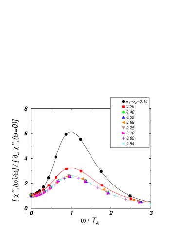
Figure 4: $\chi^{\prime\prime}_{\perp}(\omega)/\omega$ as a function of $\omega/T_{A}$.

To compare results for our model with that of the single bath DTLS, we have calculated $\chi^{{}^{\prime\prime}}_{\perp}(\omega)$ for $\alpha_{1}=0.59$ and $\alpha_{2}=0$ and compared with the case where $\alpha_{1}=\alpha_{2}=0.59$. The result is shown in Fig.5. Notice that in the DTLS case there is no trace of the peak in the susceptibility indicating that the relaxation of the spin is completely overdamped. However, in the isotropic case one finds a well defined peak even when the coupling to the environment is large, indicating that the spin still keeps memory of the tunneling splitting, even when strongly interacting with the bath. This is a clear demonstration of the effect of frustration of decoherence.

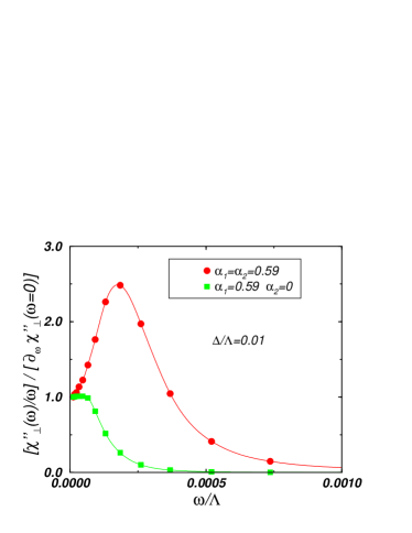
Figure 5: $\chi^{\prime\prime}_{\perp}(\omega)/\omega$ as a function of $\omega/\Lambda$.

III.2 Analytic Results

The RG results of section II show that the transverse couplings of the impurity to the environment always flow to $\alpha\to 0$ indicating that a perturbative approach should give a sensible result. When $\alpha=0$ the ground state of the problem is an eigenstate of $S_{3}$ and therefore the transverse susceptibility has a Dirac delta peak at $\omega=\Delta$, that is, zero relaxation rate, $\tau^{-1}=0$. In order to obtain a finite relaxation one makes use of the Bloch equations Abragam-01 for the expectation values of the spin operators, $M_{i}=\langle S_{i}\rangle$:

$$\frac{d\vec{M}}{dt}=\frac{\Delta}{2}\vec{M}\times\vec{z}-\frac{M_{1}\vec{x}+M_{2}\vec{y}}{T_{2}}-\frac{M_{3}\vec{z}}{T_{1}},$$

where $1/T_{2}$ is the transverse and $1/T_{1}$ is the longitudinal relaxation rates. It is straightforward to write a second order differential equation for $M_{1}(t)$:

$$\frac{d^{2}M_{1}}{dt^{2}}+\frac{2}{T_{2}}\frac{dM_{1}}{dt}+\left(\frac{\Delta^{2}}{4}+\frac{1}{T_{2}^{2}}\right)M_{1}=0\,,$$

implying that the transverse correlation function has the form:

$$\frac{\chi_{\perp}^{\prime\prime}\left(\omega\right)}{\omega} \propto \frac{2/T_{2}}{\left(\omega^{2}-\Delta^{2}/4-1/T_{2}^{2}\right)^{2}+4\omega^{2}/T_{2}^{2}}\,.$$ (25)

In appendix C.3 we derive these results using a random phase approximation (RPA) and improve on them by replacing the bare values of the parameters by their renormalized RG value:

$$\frac{\chi^{{}^{\prime\prime}}_{\perp}(\omega)}{\omega}=\frac{[\arctan(T_{A}\tau)]^{-1}T_{A}/\tau}{\left(\omega^{2}-(T_{A})^{2}-1/\tau^{2}\right)^{2}+4\omega^{2}/\tau^{2}}\,,$$ (26)

where

$$\tau^{-1}\approx\frac{\pi}{2}(\alpha^{*})^{2}T_{A}\,.$$ (27)

Notice that (26) reduces to a Dirac delta function at $\omega=\Delta$ as $\alpha(0)\to 0$, as expected. We find that this approximation is good for $\omega\ll T_{A}$ and also describes well the NRG results for all $\omega<\Lambda_{0}$ when $\Lambda_{0}>T_{A}\gg\Lambda_{0}\alpha^{*}$. In the zero frequency limit (26) reduces to

$$\chi^{{}^{\prime\prime}}_{\perp}(\omega=0)\approx(\alpha^{*})^{2}\omega/(T_{A})^{2}+{\cal O}[(\alpha^{*})^{4}]$$ (28)

and the Kramers-Kronig relation immediately leads to real part of the susceptibility:

$$\chi^{{}^{\prime}}_{\perp}(\omega\approx 0) = \pi/[8T_{A}(1+(\alpha^{*})^{4})\arctan(1/(\alpha^{*})^{2})]$$ (29)

$$\approx 1/(4T_{A})+{\cal O}[(\alpha^{*})^{2}].$$

Although the RPA result gives good results in certain regimes it fails in the asymptotic cases. In those regimes a new approach has to be developed. For that purpose we will use the criteria of renormalizability of the theory in order to calculate the susceptibility. If we knew the exact $\beta$-functions of the theory,

$$\beta_{i}(\{\alpha\})=\frac{d\alpha_{i}}{d\ell},$$ (30)

one could in principle integrate the exact RG flow in order to obtain the exact result. However, we only have access to the perturbative result (16) that indicates that there is no other fixed points in the problem. The question is whether these results are valid in other regimes.

Let us consider some limiting cases of the problem at hand. Firstly consider the special situation where $\alpha\left(0\right)=\alpha_{1}\left(0\right)=\alpha_{2}\left(0\right)$ and there is no magnetic field, $\Delta=0$ ($h\left(0\right)=0$). In this case the Hamiltonian of the problem can be written, from (6), as:

$$H_{\mathtt{eff}} = \int dx\sum_{\alpha=1,2}\left(\partial_{x}\phi_{\alpha}(x)\right)^{2}-\sqrt{8\pi\alpha}\partial_{x}\phi_{1}(0)S_{1}$$ (31)

$$- \sqrt{8\pi\alpha}\partial_{x}\phi_{2}(0)S_{2}.$$

From the renormalization group equations, Eqs. (17), we find:

$$\beta(\alpha)=\frac{d\alpha}{d\ell}=-2\alpha^{2}+{\cal O}[\alpha^{3}].$$ (32)

At finite temperature $T\ll\Lambda$ the RG flow is cut-off by the temperature and we can write $d\ell\approx-dT/T$ and use the temperature as the cut-off. We can solve (32) for $\alpha$ as a function of $T$ at once:

$$\alpha(T)\approx{\frac{\alpha_{0}}{1+2\alpha_{0}\ln(\Lambda_{0}/T)}}$$ (33)

When $T\to 0$ one finds:

$$\alpha(T)\approx{\frac{1}{2\ln(\Lambda_{0}/T)}},$$ (34)

which is independent of $\alpha(0)$ in agreement with (20).

We first consider the susceptibility at finite $T$ and zero frequency,

$$\chi(T,\Lambda,\alpha_{0})={\frac{1}{4T}}\,g(T/\Lambda,\alpha_{0}),$$ (35)

where $g(x)$ is a dimensionless function. Since the theory is renormalizable, the susceptibility should obey the Callan-Symanzik (CS) equation amit :

$$\left[\Lambda{\frac{\partial}{\partial\Lambda}}+\beta(\alpha){\frac{\partial}{\partial\alpha}}+2\gamma(\alpha)\right]g(\alpha,T/\Lambda)=0\,,$$ (36)

where $\gamma(\alpha)$ is the anomalous dimension associated with the operator $\sigma_{1}$. Equation (36) expresses the fact that a change in the cut-off, $\Lambda$, can be exactly compensated for by a change in the bare coupling, $\alpha$, together with a rescaling of the susceptibility. The most general solution of (36) is:

$$g(\alpha,T/\Lambda)=\exp\left\{\int_{\alpha_{0}}^{\alpha(T)}[2\gamma(\alpha)/\beta(\alpha)]d\alpha\right]\,h[\alpha(T)],$$ (37)

where $h(x)$ is an arbitrary function of the renormalized coupling. We can rewrite (37) in a slightly different form:

$$g(T)=\exp\left[\int_{\alpha_{0}}^{1}[2\gamma(\alpha)/\beta(\alpha)]d\alpha\right]\,\,\phi[\alpha(T)],$$ (38)

where we have introduce a new function $\phi[\alpha]$ and used that

$$\exp\left[\int_{1}^{\alpha(T)}[2\gamma(\alpha)/\beta(\alpha)]d\alpha\right]$$

is by itself some (in general unknown) function of $\alpha(T)$ and we have absorbed this term into the function $h(\alpha(T))$. Hence a non-zero anomalous dimension implies some residual explicit dependence of $g(T)$, and hence $\chi(T)$, on the bare coupling $\alpha_{0}$ in addition to its implicit dependence on $\alpha_{0}$ through the renormalized coupling. Notice from (34) that $\alpha(T)$ becomes small at low $T$ and therefore one can expand $\phi(\alpha(T))$ in a power series in $\alpha(T)$. In this case, replacing (38) into (35) we find:

$$\chi(T)={\frac{1}{4T}}\exp\left[\int_{\alpha_{0}}^{1}[2\gamma(\alpha)/\beta(\alpha)]d\alpha\right]\sum_{n}\,b_{n}\,\alpha^{n}(T),$$ (39)

where $b_{n}$ are the coefficients of the expansion of $\phi[\alpha]$.

Eq. (39) is formally exact. However, one does not know the anomalous dimension a priori. One way to go about this is to compare the exact result (39) with the perturbative result obtained in leading order in $\alpha_{0}$. In appendix C we show that perturbation theory gives:

$$\chi(T)={\frac{1}{4T}}[1+2\alpha_{0}\ln(T/\Lambda_{0})+{\cal O}[\alpha_{0}^{2}]\,.$$ (40)

Replacing (34) in (39) and comparing with (40) we find that $b_{0}=0$, $b_{1}=1$ and

$$\int_{\alpha_{0}}^{1}[2\gamma(\alpha)/\beta(\alpha)d\alpha]\approx-\ln(\alpha_{0})\,.$$ (41)

The coefficient of $2$ in front of the second term in (40) is crucial. Note that what fixes the definition of $\alpha$ is the RG equation, Eq. (32). Since $\beta(\alpha)\approx-2\alpha^{2}$, we see that:

$$\gamma(\alpha)=-\alpha+{\cal O}[\alpha^{3}]\,,$$ (42)

is the value of the anomalous dimension in leading order in $\alpha$. Therefore, we have concluded that

$$\chi(T)\approx{\frac{1}{8T\alpha_{0}\ln(\Lambda_{0}/T)}}\,,$$ (43)

when $T\to 0$. This result is expected to be true even at very low $T$ when $\alpha_{0}\ln(\Lambda/T)\geq 1$. Suppose that the bare coupling, $\alpha_{0}$ is not small. What can we say from the RG in this case? As long as we consider very low $T$ where $\alpha(T)\ll 1$ so that $\phi(\alpha(T))\approx\alpha(T)$, we have:

$$\chi(T)\approx\exp\left[\int_{\alpha_{0}}^{1}[2\gamma(\alpha)/\beta(\alpha)\right]{\frac{1}{8T\ln(\Lambda_{0}/T)}}.$$ (44)

The first factor is some unknown function of the bare coupling but the $T$ dependence is the same as before.

Now consider the susceptibility at $T=0$ but finite frequency. Once again, thanks to the renormalizability of the theory $\chi^{\prime\prime}(\omega)$ obeys the same CS equation with the same $\beta$-function and the same anomalous dimension, $\gamma(\alpha)$. This anomalous dimension is a property of the spin operator $\sigma_{1}$ and must be the same for either finite $T$ and $\omega=0$ or finite $\omega$ and $T=0$. Therefore, following the earlier discussion it must have the form:

$$\chi^{\prime\prime}(\omega,\Lambda,\alpha_{0})=\exp\left[\int_{\alpha_{0}}^{1}[2\gamma(\alpha)/\beta(\alpha)\right]{\frac{1}{\omega}}\,F(\alpha(\omega)).$$ (45)

The function $F(\alpha(\omega))$ is not necessarily the same as $\phi(\alpha(T))$ and, in general, is unknown. However, the first factor, giving the explicit dependence on $\alpha_{0}$ in a perturbative expansion, should be exactly the same as in the previous calculation of $\alpha(T)$. Thus, if $\alpha_{0}\ll 1$, we must have:

$$\chi^{\prime\prime}(\omega,\Lambda,\alpha_{0})={\frac{1}{\omega\alpha_{0}}}\,F(\alpha(\omega)).$$ (46)

Again, we perform ordinary perturbation theory for $\chi^{{}^{\prime\prime}}(\omega)$ in powers of $\alpha_{0}$ and improve the perturbative result with the RG by matching it to (46) by expanding in powers of $\alpha(\omega)$. Since we already know $\beta(\alpha)$ and $\gamma(\alpha)$, the result must have a rather restricted form to be a solution of the CS equation. The susceptibility at finite frequency is given by Eq. (69):

$$\chi^{\prime\prime}(\omega,\Lambda,\alpha_{0})\approx{\frac{1}{\omega}}\left[\alpha_{0}-4\alpha_{0}^{2}\ln(\Lambda_{0}/\omega)+{\cal O}(\alpha_{0}^{3})\right].$$ (47)

This result is consistent with the RG form of Eq. (46) if we assume that:

$$F(\alpha(\omega)) \approx \alpha^{2}(\omega)\,,$$

$$\approx \alpha_{0}^{2}-4\alpha_{0}^{3}\ln(\Lambda_{0}/\omega).$$

Having found the function $F(\alpha(\omega))$ at small $\alpha(\omega)$ we can now invoke the RG. In particular, for small bare coupling and small $\omega$ we have:

$$\chi^{\prime\prime}(\omega)\approx{\frac{1}{4\alpha_{0}\omega\ln^{2}(\Lambda_{0}/\omega)}}.$$ (49)

Even if the bare coupling is not small, but we go to small enough $\omega$ so that $\alpha(\omega)\ll 1$, the RG implies that:

$$\chi^{\prime\prime}(\omega)\approx\exp\left[\int_{\alpha_{0}}^{1}2\gamma(\alpha)/\beta(\alpha)d\alpha\right]{\frac{1}{4\omega\ln^{2}(\Lambda_{0}/\omega)}},$$ (50)

where the first term in an unknown function of the bare coupling constant. Thus, eqs. (44) and (49) give the temperature and frequency behavior of the susceptibility for, $\alpha^{*}\ll 1$, $T_{A}\ll\Lambda_{0}\alpha^{*}$, and in the frequency and temperature range $T_{A}\ll\omega,T\ll\Lambda_{0}$. When these conditions are satisfied the ratio,

$$\frac{\chi^{\prime\prime}(\omega,T=0)}{\chi(T)}=\frac{2T}{\omega}\frac{\ln(\Lambda_{0}/T)}{\ln^{2}(\Lambda_{0}/\omega)}\,,$$ (51)

is universal.

IV Discussion and Conclusions

Decoherence can be defined as the unavoidable evolution of the total state of the system and the environment towards an entangled state. This is a dynamical definition of decoherence, and clearly shows the conceptual difference between dissipation (that involves the transfer of energy from the subsystem to the environment) and decoherence. An important concept in the study of decoherence is the notion of a preferred basis: every time that a system interacts with an environment, a set of states is naturally selected by the form of the interaction. The text book example is given by the exactly solvable modelW99 ; BHP02

$$H_{deco} = \sum_{k>0}ka_{k}^{\dagger}a_{k}+i\frac{\lambda_{1}}{\sqrt{2L}}S_{1}\sum_{k>0}\sqrt{k}(a_{k}-a_{k}^{\dagger}).$$

Although this model does not have any dissipative mechanism, the two level system experience strong decoherence. Suppose that the system is prepared at time $t=0$ as a direct product of the bath and the two level system:

$$\rho(t=0) = \rho_{bath}(t=0)\otimes\rho_{\vec{S}}(t=0),$$

where $\rho_{bath}$ and $\rho_{\vec{S}}$ are respectively the density matrices of bath and the two level system. A natural basis choice for the two level system is $S_{1}$. If we further suppose that the two level system is prepared in a state of $S_{2}$, then at $t=0$ the reduced density matrix,

$$\rho_{R}(t=0) = tr_{bath}\left[\rho_{bath}(t=0)\otimes\rho_{\vec{S}}(t=0)\right],$$

has off-diagonal matrix elements indicating that the system is coherent. As the system evolves in time the off-diagonal elements decay very fast due to the entanglement of $\vec{S}$ and the bath degrees of freedom. As $t\to\infty$ only the diagonal elements of the reduced density matrix of the system remain, and we say that the system “decoheres” to the preferred basis of $S_{1}$.

With this example in mind is now simple to understand the effects that we described in this manuscript. Consider the Hamiltonian (5). In this case it is no longer possible to define a preferred basis for the two level system. The entanglement of $\vec{S}$ with each one of the baths is suppressed by the other, and as a result the decoherence phenomena is frustrated. This physical picture shows the true meaning of our results, the “quantum frustration” is the lack of a preferred basis for the system of interest.

The quantum frustration of decoherence can be also understood as a result of a version of Coleman’s or Mermin-Wagner’s theorem coleman . When $\alpha_{1}=\alpha_{2}$ there is a $U(1)$ symmetry in impurity problem. Hence, one has an effective $(1+1)$ dimensional field theory with $U(1)$ symmetry so this symmetry cannot be spontaneously broken even at $T=0$. In fact, because one has a single boundary degree of freedom, one can also think of the problem as an almost $(0+1)$ dimensional field theory. So it is a rather remarkable fact that even the $Z_{2}$ symmetry which remains when $\alpha_{2}=0$ can be spontaneously broken, as in the case of the DTLS. The $U(1)$ symmetry would have to be spontaneously broken in a phase in which the spin is localized in an eigenstate of either $S_{1}$ or $S_{2}$. Quantum mechanics prevents that from happening.

One can ask how generic this result really is. For quantum frustration to occur the coupling constants with all the baths must be identical. This can be achieved when the role of the two baths is played by two Goldstone modes, resulting from the spontaneous breaking of a continuous symmetry, such that the residual unbroken symmetry rotates the two Goldstone modes into each other. When the couplings are not exactly equal quantum frustration occurs up to a certain energy scale below which one of the heat baths takes over and one obtains the standard decoherence problem in dissipative ohmic systems. In terms of Fig.1 it means that the asymptotic flow is the one for either $\alpha_{1}=0$ or $\alpha_{2}=0$. In summary, quantum frustration of decoherence is a general phenomena. It has clear implications to quantum/classical transition and measure theory. Moreover it is potentially important to the development of technologies where decoherence is a fundamental issue as in the case of quantum communication and quantum computation.

In summary, we have studied a model of quantum frustration of decoherence in open systems. Contrary to standard dissipative models with ohmic dissipation, the non-commutative nature of spin operators lead to a frustration of decoherence. We have shown that while in a DTLS the spin dynamics becomes overdamped at large couplings with a heat bath, in a system with quantum frustration it is always underdamped and the system keeps the memory of its quantum nature. Using perturbative RG calculations we have shown that at large couplings with the bath the transverse spin susceptibility shows scaling with a characteristic energy scale $T_{A}$, the analogous of the Kondo temperature in the DTLS, that separates the region of strong to weak coupling. We have supported our claims with NRG calculations and have calculated the frequency and temperature dependence of the transverse susceptibility using the renormalizability of the theory. Our results may be applicable to a large class of problems where decoherence plays a fundamental role.

Appendix A Impurity spin in a magnetically ordered environment

In this appendix we will show how quantum frustration can arise in the context of a magnetic impurity in a magnetic environment prl . Let us consider a magnetic environment describe by the quantum Heisenberg Hamiltonian in the presence of an impurity:

$$H = J\sum_{\langle i,j\rangle}\vec{s}_{i}\cdot\vec{s}_{j}+\lambda\,\vec{S}\cdot\vec{s}_{0},$$ (52)

where $J$ is the magnetic exchange between nearest neighbor spins $\vec{s}_{i}$ located on a lattice site $\vec{R}_{i}$ in $d$ dimensions, $\lambda$ is the coupling between the environmental spins and an impurity spin $\vec{S}$ located at the origin of the coordinate system. In what follows we will consider the antiferromagnetic case of $J>0$ although the ferromagnetic case ($J<0$) can be studied in an analogous way.

The partition function of the problem in spin coherent state path integral can be written as fradkin :

$$Z = \int D\vec{N}\,\delta(\vec{N}^{2}-1)\int D\vec{n}\,\delta(\vec{n}^{2}-1)\,\,e^{-iS_{\mathtt{B}}(\vec{N})-S(\vec{N},\vec{n})}$$

where $\vec{N}$ represents the impurity spin and $\vec{n}(\vec{r})$ the environmental spin field, $S_{\mathtt{B}}$ is the Berry’s phase,

$$S = \int d\tau d\vec{r}\left\{\frac{1}{2g}\left[\left(\partial_{\tau}\vec{n}(\tau,\vec{r})\right)^{2}+c^{2}\left(\nabla\vec{n}(\tau,\vec{r})\right)^{2}\right]\right.$$ (53)

$$+ \left.\lambda\delta\left(\vec{r}\right)\vec{n}(\tau,\vec{r})\cdot\vec{N}\left(\tau\right)\right\},$$

is the action of the problem where $g=c^{2}/\rho_{s}$ is the coupling constant ($c=2\sqrt{d}Jas$ is the spin wave-velocity and $\rho_{s}=Js^{2}a^{2-d}$ is the spin stiffness, $a$ is the lattice spacing and $s$ is the value of the environmental spin).

Assume that the $O(3)$ symmetry of the model is spontaneously broken so that the field $\vec{n}$ orders. In this case we can write:

$$\vec{n}\left(\tau,\vec{r}\right) \approx \left(\varphi_{1}\left(\tau,\vec{r}\right),\varphi_{2}\left(\tau,\vec{r}\right),1\right),$$ (54)

where $\varphi_{1,2}$ are small fluctuating fields corresponding to the two Goldstone modes of the antiferromagnet. A possibility that is not considered in this work is associated with the formation of a spin texture around the impurity spin. In a classical spin system a spin texture can be formed in the bulk spins due to the presence of strong and/or anisotropic interactions. The spin texture can follow the impurity as it tunnels invalidating the methods used here (an instanton calculation is required to take into account the collective nature of the texture). The results in this appendix are only valid if no spin texture is formed around the magnetic impurity.

In the ordered phase the Berry’s phase term is unimportant and can be dropped. Using Eq. (54) the action (53) reads,

$$S \approx \sum_{\alpha=1,2}\int d\tau d\vec{r}\left\{\frac{1}{2g}\left[\left(\partial_{\tau}\varphi_{\alpha}(\tau,\vec{r})\right)^{2}+c^{2}\left(\nabla\varphi_{\alpha}(\tau,\vec{r}\right)^{2}\right]\right.$$ (55)

$$+ \left.\lambda\delta\left(\vec{r}\right)\varphi_{\alpha}(\tau,\vec{r})\cdot N_{\alpha}(\tau)+\lambda N_{3}\left(\tau\right)\right\}.$$

We see that the action for the fields $\varphi_{1,2}$ is quadratic and therefore these fields can be traced out of the problem exactly. In this case the effective action for the impurity spin becomes in Fourier space:

$$S_{\mathtt{eff}} \approx \frac{g\lambda^{2}}{2}\sum_{\alpha=1,2}\int d\omega d\vec{k}\frac{N_{\alpha}(\omega)N_{\alpha}(-\omega)}{\omega^{2}+c^{2}{k}^{2}}$$

$$+ \lambda\int d\tau N_{3}\left(\tau\right).$$

As we should expect from the spherical symmetry of the problem, the angular dependence in $\vec{k}$ can be integrated and we finally obtain

$$S_{\mathtt{eff}} \approx \frac{\alpha^{2}}{\Gamma(d-1)}\sum_{\alpha=1,2}\int_{-\infty}^{+\infty}d\omega\left[\int_{0}^{\infty}dq\,\frac{q^{d-1}}{\omega^{2}+q^{2}}\right]N_{\alpha}(\omega)N_{\alpha}(-\omega)\,$$ (56)

$$+ \lambda\int d\tau N_{3}\left(\tau\right)\,,$$

where $q=ck$, and

$$\alpha^{2}=\frac{g\Gamma(d-1)\lambda^{2}}{2^{d+2}\pi^{\left(d-2\right)/2}\Gamma\left(d/2\right)c^{d}},$$

where $\Gamma(x)$ is a gamma function. Integrating (56) over $q$ and Fourier transforming back the frequencies to imaginary time we find:

$$S_{\mathtt{eff}} \approx \alpha^{2}\sum_{\alpha=1,2}\int d\tau\int d\tau^{\prime}\frac{N_{\alpha}(\tau)N_{\alpha}(\tau^{\prime})}{|\tau-\tau^{\prime}|^{d-1}}$$ (57)

$$+ \lambda\int d\tau N_{3}\left(\tau\right),$$

which shows that the impurity interact in imaginary time through a long-range interaction that decays like $1/\tau^{d-1}$.

The action (57) can be simplified by introducing a Hubbard-Stratanovich field that splits the interaction term. This can be done with the introduction of one-dimensional bosonic fields defined as:

$$\phi_{\alpha}\left(x,\tau\right) = \frac{T}{\sqrt{2L}}\sum_{q>0}\sum_{\omega_{n}}\frac{e^{iqx+i\omega_{n}\tau}}{\sqrt{q}}\phi_{\alpha}^{*}\left(q,\omega_{n}\right)$$

$$+ \frac{e^{-iqx+i\omega_{n}\tau}}{\sqrt{q}}\phi_{\alpha}\left(q,\omega_{n}\right),$$

$L\to\infty$ is the size of the one-dimensional line. Using these new fields the action (57) can be written as:

$$S_{\mathtt{eff}} = \sum_{\alpha=1,2}T\sum_{q>0}\sum_{\omega_{n}}\left[i\omega_{n}+q\right]\phi_{\alpha}^{*}\left(q,\omega_{n}\right)\phi_{\alpha}\left(q,-\omega_{n}\right)$$ (58)

$$+ \alpha\left|q\right|^{\frac{d-1}{2}}\left[\phi_{\alpha}^{*}\left(q,\omega_{n}\right)N_{\alpha}(\omega_{n})+\phi_{\alpha}\left(q,\omega_{n}\right)N_{\alpha}(-\omega_{n})\right]$$

$$+ \lambda\int d\tau N_{3}\left(\tau\right).$$

It is easy to see that the trace over the bosonic fields reproduces (57). It is straightforward to see that in $d=3$ the above action reduces to (6).

Appendix B RG equations

In this appendix we will derive the RG equations (12). From equation (9a) we have:

$$\langle A_{1}^{\pm}\rangle_{>} = \langle e^{\mp i\sqrt{8\pi\alpha_{1}}(\phi_{1,<}\left(x=0\right)+\phi_{1,>}\left(x=0\right))}S^{\pm}\rangle_{>}$$ (59)

$$= A_{1,<}^{\pm}\langle e^{\mp i\sqrt{8\pi\alpha_{1}}\phi_{1,>}\left(x=0\right)}\rangle_{>}$$

$$= A_{1,<}^{\pm}e^{-\alpha_{1}d\ell}\approx A_{1,<}^{\pm}(1-\alpha_{1}d\ell)\,.$$

Substituting (59) in (10) one obtains a term of the form:

$$\delta\tau e^{d\ell}\Delta e^{-\alpha_{1}d\ell}A_{1,<}^{m_{j}}=\delta\tau\Delta(\ell+d\ell)A_{1,<}^{m_{j}}\,,$$ (60)

where we have used that, by rescaling $\omega\to\omega/b$ (with $b=e^{d\ell}\approx 1+d\ell$) one has $\tau\to b\tau$. Hence,

$$\Delta(\ell+d\ell)=\Delta(\ell)[1+(1-\alpha_{1})d\ell]\,,$$ (61)

and defining the dimensionless coupling, $h(\ell)=\Delta(\ell)/\Lambda$, one obtains (12b).

Analogously, from (9b) we have:

$$\langle B_{1}^{\pm}\rangle_{>} = B_{1,<}^{\pm}e^{-d\ell}\langle e^{\mp i\sqrt{8\pi\alpha_{1}}\phi_{1}\left(x=0\right)}\rangle_{>}$$ (62)

$$= B_{1,<}^{\pm}e^{-(1+\alpha_{1})d\ell}$$

$$\approx B_{1,<}^{\pm}[1-(1+\alpha_{1})d\ell]\,,$$

where we have used that $\partial_{x}\to b^{-1}\partial_{x}$ since $k\to k/b$. Replacing (62) into the second term in the r.h.s. of (10):

$$\delta\tau\sqrt{\alpha_{2}}e^{-\alpha_{1}d\ell}B_{1,<}^{m_{j}}\left(\tau_{j}\right)=\delta\tau\sqrt{\alpha_{2}(\ell+d\ell)}B_{1,<}^{m_{j}}\,,$$ (63)

and hence we write:

$$\alpha_{2}(\ell+d\ell)=\alpha_{2}(\ell)e^{-2\alpha_{1}d\ell}\approx\alpha_{2}(\ell)(1-2\alpha_{1}d\ell)\,,$$ (64)

leading to equation (12a).

Appendix C Perturbation Theory

In this appendix we show how to derive the perturbative expansion for the transverse susceptibility:

$$\mathcal{S}\left(\tau\right) = \left\langle T_{\tau}S_{1}\left(\tau\right)S_{1}\left(0\right)\right\rangle\,.$$

C.1 Static susceptibility $\omega=0$ and $h=0$

Firstly, let us consider the case of arbitrary $\alpha_{2}$ but small $\alpha_{1}$ (the case of arbitrary $\alpha_{1}$ and $\alpha_{2}\ll 1$ is completely analogous). This regime can be obtained by using eq. (7):

$$\bar{H_{2}} = U_{2}^{-1}H_{\mathtt{eff}}U_{2}$$

$$= H_{0}-\sqrt{2\pi}\alpha_{1}\partial_{x}\phi_{1}e^{-i\sqrt{8\pi\alpha_{2}}\phi_{2}\left(0\right)}S^{+}+\mathtt{h}.\mathtt{c}.$$

In this rotated basis, $\mathcal{S}\left(\tau\right)$ has a simple form:

$$\mathcal{S}\left(\tau\right) = \frac{1}{4}\left\langle T_{\tau}\left(A_{2}^{+}\left(\tau\right)+A_{2}^{-}\left(\tau\right)\right)\left(A_{2}^{+}\left(0\right)+A_{2}^{-}\left(0\right)\right)\right\rangle,$$

where

$$A_{2}^{\pm}\left(\tau\right) = e^{\mp i\sqrt{8\pi\alpha_{2}}\phi_{2}\left(0,\tau\right)}S^{\pm}\left(\tau\right).$$

The leading order terms in an expansion in powers of $\alpha_{1}$ at $T=0$ can be immediately obtained from the bosonic propagator:

$$\mathcal{S}\left(\tau\right) \approx \frac{1}{4}\left|D\tau\right|^{-2\alpha_{2}}+{\cal O}[\alpha_{1}\alpha_{2}]\,,$$ (65)

where $D$ is a short time cut-off. We can use the standard conformal transformation to promote this result to a finite temperature expression,

$$\mathcal{S}\left(\tau\right)\approx\frac{1}{4}\left(\frac{D}{T\pi}\sin\left|\pi T\tau\right|\right)^{-2\alpha_{2}}+{\cal O}[\alpha_{1}\alpha_{2}]\,.$$

Expanding the above expression for $\alpha_{2}\ll 1$ gives:

$$\mathcal{S}\left(\tau\right)\approx\frac{1}{4}\left[1-2\alpha_{2}\ln\left(\frac{D}{T\pi}\sin\left|\pi\tau T\right|\right)+{\cal O}[\alpha_{1}\alpha_{2},\alpha_{2}^{2}]\right].$$

To this order, the susceptibility can be calculated immediately:

$$\chi\left(T\right) = \int_{0}^{1/T}d\tau\mathcal{S}\left(\tau\right)$$ (66)

$$\approx \frac{1}{4T}\left[1-\frac{2\alpha_{2}}{T}\ln\left(\frac{D}{2\pi T}\right)+{\cal O}[\alpha_{1}\alpha_{2},\alpha_{2}^{2}]\right]\,.$$

For completeness, let us re-obtain this result by a direct perturbative calculation in second order in $\alpha_{2}$:

$$\mathcal{S}\left(\tau\right) \approx 8\pi\alpha_{2}\int_{\tau}^{1/T}d\tau_{1}\int_{0}^{\tau}d\tau_{2}\left[\left\langle T_{\tau}\sigma_{2}\left(\tau_{1}\right)\sigma_{1}\left(\tau\right)\sigma_{2}\left(\tau_{2}\right)\sigma_{1}\left(0\right)\right\rangle-\left\langle T_{\tau}\sigma_{1}\left(\tau\right)\sigma_{1}\left(0\right)\right\rangle\left\langle T_{\tau}\sigma_{2}\left(\tau_{1}\right)\sigma_{2}\left(\tau_{2}\right)\right\rangle\right]\left\langle T_{\tau}\partial\phi_{2}\left(\tau_{1}\right)\partial\phi_{2}\left(\tau_{2}\right)\right\rangle$$

$$= -\frac{\pi\alpha_{2}}{8}\int_{\tau}^{1/T}d\tau_{1}\int_{0}^{\tau}d\tau_{2}\left\langle\partial\phi_{2}\left(\tau_{1}\right)\partial\phi_{2}\left(\tau_{2}\right)\right\rangle.$$

Using the finite temperature propagator,

$$\left\langle\partial\phi_{2}\left(\tau_{1}\right)\partial\phi_{2}\left(\tau_{2}\right)\right\rangle = \frac{1}{4\pi}\frac{1}{\left[\frac{1}{\pi T}\sin\left[\pi T\left|\tau_{2}-\tau_{1}\right|\right]\right]^{2}},$$

we obtain

$$\mathcal{S}\left(\tau\right) \approx -\frac{\alpha_{2}}{4}\int_{\tau+\frac{1}{D}}^{1/T}d\tau_{1}\int_{0}^{\tau}d\tau_{2}\frac{1}{\left[\frac{1}{\pi T}\sin\left[\pi T\left|\tau_{2}-\tau_{1}\right|\right]\right]^{2}}$$

$$\approx \frac{\alpha_{2}}{2}\left[\ln\left(\frac{\pi T}{D}\right)-\ln\left(\sin\left|\pi T\tau\right|\right)\right]+{\cal O}[\alpha_{1}\alpha_{2},\alpha_{2}^{2}]\,,$$

in agreement with (66).

C.2 Dynamic susceptibility $\omega\neq 0$ at $T=0$ and $h=0$

The finite frequency calculation is a little more tedious than the previous one. We would like to obtain the correlation function in fourth order in the coupling constants. From Eq. (65) we already know part of the result,

$$\mathcal{S}\left(\tau\right)=\frac{1}{4}-\frac{1}{2}\alpha_{2}\ln\left|D\tau\right|+\frac{1}{2}\alpha_{2}^{2}\ln^{2}\left|D\tau\right|+{\cal O}[\alpha_{1}\alpha_{2},\alpha_{2}^{3}].$$ (67)

The remaining contribution to the correlation function is a term proportional to $\alpha_{1}\alpha_{2}$. A convenient way to derive this contribution is to use Eq. (7a) and compute the result to all orders in $\alpha_{1}$ but for $\alpha_{2}\ll 1$. In second order in $\alpha_{2}$ we need to calculate:

$$\delta\mathcal{S}\left(\tau\right) = \frac{1}{4}+2\pi\alpha_{2}\int d\tau_{1}d\tau_{2}\left\langle T_{\tau}S_{3}\left(\tau\right)B_{1}^{+}\left(\tau_{1}\right)B_{1}^{-}\left(\tau_{2}\right)S_{3}\left(0\right)\right\rangle-\pi\alpha_{2}\int d\tau_{1}d\tau_{2}\left\langle T_{\tau}B_{1}^{+}\left(\tau_{1}\right)B_{1}^{-}\left(\tau_{2}\right)\right\rangle.$$

From this point, it is straightforward to obtain the correlation function and the susceptibility at finite frequency:

$$\delta\mathcal{S}\left(\tau\right) = \frac{1}{4}-\frac{\alpha_{2}}{4D^{2\alpha_{1}}}\frac{1}{\left[1+2\alpha_{1}\right]\alpha_{1}}\times$$

$$\times \left[\frac{1}{\left|\frac{1}{D}\right|^{2\alpha_{1}}}-\frac{1}{\left|\tau\right|^{2\alpha_{1}}}\right],$$

$$\delta\chi\left(i\omega_{n}\neq 0\right) = \frac{\alpha_{2}^{2}}{\left[1+2\alpha_{1}\right]2\alpha_{1}D^{2\alpha_{1}}\left|\omega_{n}\right|^{1-2\alpha_{1}}}\times$$

$$\times \left\{\Gamma\left(1-2\alpha_{1}\right)\sin\left[\pi\alpha_{1}\right]\right\}.$$

Expanding for $\alpha_{1}\ll 1$ and $\alpha_{1}\ln(D/|\omega_{n}|)\ll 1$ we find:

$$\delta\chi\left(i\omega_{n}\neq 0\right) = \frac{\pi\alpha_{1}\alpha_{2}}{\left|\omega_{n}\right|}\left[\left(\mathcal{C}-1\right)+\ln\left|\frac{\omega_{n}}{D}\right|\right],$$ (68)

where $\mathcal{C}\approx 0.57772$ is the Euler-Gamma constant. The susceptibility in fourth order in the coupling constants is the sum of Eq. (68) and the Fourier transform of Eq. (67),

$$\chi\left(i\omega_{n}\right) = \frac{1}{4}\delta\left(\omega_{n}\right)+\frac{\pi\alpha_{2}}{2}\frac{1}{\left|\omega_{n}\right|}\left[1-2\left(\alpha_{2}+\alpha_{1}\right)\ln\left(\frac{D}{\left|\omega_{n}\right|}\right)+2\mathcal{C}\alpha_{2}+2\left(\mathcal{C}-1\right)\alpha_{1}+{\cal O}[\alpha_{2}^{2},\alpha_{1}^{2}]\right].$$ (69)

C.3 Asymptotic regime of $h\to\infty$

We represent the spin variables in (31) in terms of two spinless fermions:

$$S_{1} = \left(a^{\dagger}b+b^{\dagger}a\right)/2$$

$$S_{2} = -i\left(a^{\dagger}b-b^{\dagger}a\right)/2$$

$$S_{3} = \left(a^{\dagger}a-b^{\dagger}b\right)/2$$

and add to the action an imaginary chemical potential, $i\omega_{0}=i\pi T/2.$ Working with this formalism we can use Wick’s theorem and the standard diagrammatic technique. The action is rewritten as

$$S = S_{0}\left(\phi_{1},\phi_{2}\right)+\int d\tau\,a^{*}\left(\tau\right)\left[\partial_{\tau}-\mathtt{z}\right]a\left(\tau\right)+$$

$$+ b^{*}\left(\tau\right)\left[\partial_{\tau}+\mathtt{z}^{*}\right]b\left(\tau\right)+\sqrt{2\pi}\left[\sqrt{\alpha_{1}}\partial_{x}\phi_{1}\left(0,\tau\right)\right.$$

$$- \left.i\sqrt{\alpha_{2}}\partial_{x}\phi_{2}\left(0,\tau\right)\right]a*\left(\tau\right)b\left(\tau\right)+\mathtt{h}.\mathtt{c}.\,,$$

where $\mathtt{z}=i\omega_{0}+\frac{h}{2}$. We define the following propagators,

$$\mathcal{G}_{a}^{\left(0\right)}\left(i\omega_{n}\right) = \frac{-1}{i\omega_{n}-\mathtt{z}},$$

$$\mathcal{G}_{b}^{\left(0\right)}\left(i\omega_{n}\right) = \frac{-1}{i\omega_{n}+\mathtt{z}^{*}},$$

$$\mathcal{D}_{1,2}^{\left(0\right)}\left(i\omega_{n}\neq 0\right) = -\frac{|\omega_{n}|}{2\pi}\arctan{\left(\frac{D}{|\omega_{n}|}\right)}\,,$$

for the fields $a(\tau)$, $b(\tau)$, and the boundary field $\phi_{1,2}(0,\tau)$.

From the propagators we immediately derive the zeroth order part of the susceptibility:

$$\chi_{0}\left(i\omega_{n}\right) = \frac{T}{4}\sum_{p_{n}}\mathcal{G}_{a}^{\left(0\right)}\left(i\omega_{n}+ip_{n}\right)\mathcal{G}_{b}^{\left(0\right)}\left(ip_{n}\right)$$

$$+\mathcal{G}_{b}^{\left(0\right)}\left(i\omega_{n}+ip_{n}\right)\mathcal{G}_{a}^{\left(0\right)}\left(ip_{n}\right)$$

$$= \frac{1}{4}\left(\frac{1}{i\omega_{n}+h}-\frac{1}{i\omega_{n}-h}\right)$$

$$= \frac{1}{2}\frac{h}{\omega_{n}^{2}+h^{2}}.$$

A simple perturbative calculation will fail to capture the physics and the correct behavior of the susceptibility. Following the standard prescription we will sum the infinite series of bubble diagrams in the RPA. Let us first consider the second order bubble diagrams. From the definition of the propagators and assuming $\left|\omega_{n}\right|\ll D$, we obtain:

$$\delta\chi_{1}\left(i\omega_{n}\neq 0\right) = -\frac{\pi\alpha_{1}}{2}\frac{h^{2}}{\left(\omega_{n}^{2}+h^{2}\right)^{2}}|\omega_{n}|$$

$$= -2\pi\alpha_{1}\left[\chi_{0}\left(i\omega_{n}\right)\right]^{2}|\omega_{n}|$$

$$\delta\chi_{2}\left(i\omega_{n}\neq 0\right) = \frac{\pi\alpha_{2}}{2}\frac{\omega_{n}^{2}}{\left(\omega_{n}^{2}+h^{2}\right)^{2}}|\omega_{n}|$$

$$= 2\pi\alpha_{2}\left[\chi_{0}\left(i\omega_{n}\right)\right]^{2}\left(\frac{\omega_{n}}{h}\right)^{2}|\omega_{n}|.$$

The bubble diagrams in fourth and sixth order can be calculated in a straightforward way:

$$\frac{\chi_{\mathtt{RPA}}^{\left(4\right)}\left(i\omega_{n}\right)}{\left[\chi_{0}\left(i\omega_{n}\right)\right]^{3}} = 4\pi^{2}\omega_{n}^{2}\left[\alpha_{1}^{2}-\alpha_{2}\left(\frac{\omega_{n}}{h}\right)^{2}\left(2\alpha_{1}+\alpha_{2}\right)\right]$$

$$\frac{\chi_{\mathtt{RPA}}^{\left(6\right)}\left(i\omega_{n}\right)}{\left[\chi_{0}\left(i\omega_{n}\right)\right]^{4}} = -8\pi^{3}\left|\omega_{n}\right|^{3}\left[\alpha_{1}^{3}-\alpha_{2}\left(\frac{\omega_{n}}{h}\right)^{2}\left(3\alpha_{1}^{2}\right.\right.$$

$$+ \left.\left.2\alpha_{1}\alpha_{2}+\alpha_{2}^{2}\right)+\alpha_{1}\alpha_{2}^{2}\left(\frac{\omega_{n}}{h}\right)^{4}\right]\,.$$

For $h\gg\alpha_{2}\omega_{n}$, we can simplify these results and sum the geometric series,

$$\chi_{\mathtt{RPA}}\left(i\omega_{n}\right) \approx \frac{\chi_{0}\left(i\omega_{n}\right)}{1+2\pi\alpha_{1}\left|\omega_{n}\right|\chi^{\left(0\right)}\left(i\omega_{n}\right)},$$

$$\approx \frac{\left(h/2\right)}{h^{2}+\omega_{n}^{2}+\pi h\alpha_{1}\left|\omega_{n}\right|}.$$

The zero temperature susceptibility in the RPA approximation (for low frequencies and high magnetic fields) is obtained by the analytical continuation,

$$\frac{\chi_{\mathtt{RPA}}^{\prime\prime}\left(\omega\right)}{\omega} \approx \frac{\pi}{2}\frac{\alpha^{2}_{1}h}{\left(\omega^{2}-h^{2}\right)^{2}+\pi^{2}h\alpha_{1}^{2}\omega^{2}}.$$

If we define the decoherence time

$$T_{2}^{-1}=\frac{\pi}{2}h\alpha^{2}_{1}\,,$$ (70)

we can identify the functional form obtained in Eq. (25),

$$\frac{\chi_{\mathtt{RPA}}^{\prime\prime}\left(\omega\right)}{\omega} \approx \frac{h/T_{2}}{\left(\omega^{2}-h^{2}\right)^{2}+4\omega^{2}/T_{2}^{2}},$$

that leads to (26) if one replaces:

$$h \to T_{A}$$

$$\alpha_{1} \to \alpha^{*}$$

$$T_{2}^{-1} \to \tau^{-1}=\frac{\pi}{2}T_{A}(\alpha^{*})^{2}\,.$$ (71)

References

- (1) Shin Takagi, Macroscopic quantum tunneling (Cambridge University Press, Cambridge, 2002).
- (2) Michael A. Nielsen, and Isaac L. Chuang, Quantum Computation and Quantum Information (Cambridge University Press, Cambridge, 2000).
- (3) A. O. Caldeira and A. J. Leggett. Physica, 121A, 587 (1983), A. O. Caldeira and A. J. Leggett. Annals of Physics 149, 374, (1983).
- (4) A. M. Tsvelik, and P. G. Wiegmann, Adv. Phys. 32, 453 (1983).
- (5) K. G. Wilson, Rev. Mod. Phys. 47 773 (1975); T. A. Costi in Density Matrix Renormalization, eds. I. Peschel et al. (Springer, 1999).
- (6) I. Affleck, Acta Phys. Polon. B 26, 1869 (1995).
- (7) A. J. Leggett, S. Chakravarty, A. T. Dorsey, Matthew P. A. Fisher, Anupam Garg and W. Zwerger, Rev. Mod. Phys. 59, 1 (1987).
- (8) J. L. Smith, and Q. Si, Europhys. Lett. 45 228 (1999); A. Sengupta, Phys. Rev. B 61, 4041 (2000).
- (9) A. H. Castro Neto and B. A. Jones, Phys. Rev. B 62, 14975 (2000).
- (10) F. Lesage, H. Saleur, and S. Skorik, Phys. Rev. Lett. 76, 3388 (1996).
- (11) T. A. Costi and C. Kieer, Phys. Rev. Lett. 76, 1683 (1996); T. A. Costi, G. Zarand, Phys. Rev. B 59, 12398 (1999).
- (12) A. H. Castro Neto, E. Novais, L. Borda, Gergely Zarand, and I. Affleck, Phys. Rev. Lett. 91, 096401 (2003).
- (13) See, S. Sachdev, Jou. Stat. Phys. 115, 47 (2004), and references therein.
- (14) See, Matthias Vojta, cond-mat/0412208, and references therein.
- (15) B. Nienhuis, in Phase Transition and Critical Phenomena (Academic Press, London, 1987), vol. 11, pp. 1-53.
- (16) P. W. Anderson, G. Yuval, and D. R. Hamann, Phys. Rev. B 1, 4464 (1970).
- (17) E. Novais, E. Miranda, A. H. Castro Neto and G. G. Cabrera, Phys. Rev. B, 66, 174409 (2002).
- (18) The same equation can be obtained in a straightforward way from the product operator expansion (OPE) for and (see [zarand, ]).
- (19) L. Zhu, and Q. Si, Phys. Rev. B 66, 024426 (2002); G. Zárand, and E. Demler, Phys. Rev. B 66, 024427 (2002).
- (20) Ralf Bulla, Ning-Hua Tong, and Matthias Vojta, Phys. Rev. Lett. 91, 170601 (2003).
- (21) D. J. Amit, Field Theory, the Renormalization Group and Critical Phenomena (World Scientific Publishing, 1984).
- (22) A. Abragam, The Principal of Nuclear Magnetism, (Oxford University Press, London, 1961).
- (23) U. Weiss, Quantum Dissipative Systems, (World Scientific, Singapore, 1999).
- (24) H. P. Breuer and F. Petruccione, The theory of open quantum systems, (Oxford University Press,Oxford, 2002).
- (25) E. Fradkin, Field Theories of Condensed Matter Systems, (Addison-Wesley, Redwood City, 1991).
- (26) S. Coleman, Aspects of Symmetry, (Cambridge University Press, Cambridge, 1985).