Linking physics and algorithms in the random-field Ising model

Abstract

The energy landscape for the random-field Ising model (RFIM) is complex, yet algorithms such as the push-relabel algorithm exist for computing the exact ground state of an RFIM sample in time polynomial in the sample volume. Simulations were carried out to investigate the scaling properties of the push-relabel algorithm. The time evolution of the algorithm was studied along with the statistics of an auxiliary potential field. At very small random fields, the algorithm dynamics are closely related to the dynamics of two-species annihilation, consistent with fractal statistics for the distribution of minima in the potential (“height”). For $d=1,2$, a correlation length diverging at zero disorder sets a cutoff scale for the magnitude of the height field; our results are most consistent with a power-law correction to the exponential scaling of the correlation length with disorder in $d=2$. Near the ferromagnetic-paramagnetic transition in $d=3$, the time to find a solution diverges with a dynamic critical exponent of $z=0.93\pm 0.06$ for a priority queue version and $z=0.43\pm 0.06$ for a first-in first-out queue version of the algorithm. The links between the evolution of auxiliary fields in algorithmic time and the static physical properties of the RFIM ground state provide insight into the physics of the RFIM and a better understanding of how the algorithm functions.

I Introduction

Models of materials with quenched disorder, such as spin glasses and random magnets Young (1998), typically have extremely slow dynamics in the low-temperature glassy phase, due to the existence of many metastable states separated by barriers that grow with the system size. Such exponential slowing down affects optimization methods that are modeled on the dynamics of the physical system, such as simulated annealing Kirkpatrick et al. (1983). The slow dynamics of the system prevent precise study of the equilibrium behavior. Besides using physically motivated dynamics, one can consider using combinatorial methods Alava et al. (2001); Hartmann and Rieger (2002) to compute partition functions or ground states. Some problems, such as determining the ground state of a 3D spin glass Barahona (1982) or finding the partition function for the RFIM at finite temperature, are NP-hard J. C. Angles d’Auriac et al. (1985); Sorin Istrail (1999). Though combinatorial approaches derived in computer science greatly accelerate searches for the ground state F. Barahona et al. (1988); F. Liers et al. (2004), it is difficult to study systems with more than $10^{3}$ degrees of freedom. However, many problems for disordered materials, such as computing the partition function of a 2D spin glass Barahona (1982) or finding the ground state of an RFIM sample d’Auriac et al. (1985), can be solved in time polynomial in the volume of the sample, allowing for the solution of samples with over $10^{7}$ degrees of freedom.

The push-relabel (PR) algorithm introduced by Goldberg and Tarjan Goldberg and Tarjan (1988) is directly applicable to finding the exact ground state of the RFIM and has been extensively applied to study the RFIM’s zero-temperature paramagnetic-ferromagnetic transition Barahona (1985); Ogielski (1986); Hartmann and Nowak (1999); d’Auriac and Sourlas (1997); Middleton and Fisher (2002); Hartmann and Rieger (2002); Hambrick et al. (2005); Bastea and Duxbury (1998). The running time is bound by a polynomial in the number of spins, but there is a power-law critical slowing down of the PR algorithm at the zero-temperature ($T=0$) transition Ogielski (1986); Middleton and Fisher (2002); Middleton (2002a).

This paper explores the connection between the auxiliary variables of the PR algorithm and the zero-temperature disorder-driven phase transition. We also look at the algorithm in the limit of small disorder, where the dynamics of the algorithm turn out to be closely related to annihilation processes studied in statistical physics A. D. Rutenberg (1998); F. Leyvraz and S. Redner (1992); Toussaint and Wilczek (1983).

We define the RFIM Hamiltonian, review its phases, and define the rules for the push-relabel dynamics in Sec. II. These rules describe the evolution of auxiliary fields; the dynamics of these fields leads directly to a ground state for the RFIM. Our main focus will be on the “height” or potential field. This field guides the determination of the spin-up and spin-down domains in the ground state. Given these definitions, we outline our results in Sec. III. We study the relationship of the PR algorithm to annihilation processes at low values of the disorder by studying the algorithm dynamics and final topography of this auxiliary potential surface in Sec. IV. In Sec. V, we study the topography of the potential surface for general disorder, especially near the paramagnetic-ferromagnetic transition. The primary results of the paper, especially the scaling of the running time and statistics of the potential field, are summarized in Sec. VI.

II Random-field Ising model and the push-relabel algorithm

The random-field Ising model (see, e.g., Young (1998) and references therein) captures essential features of models in statistical physics that are controlled by disorder and have “frustration”, i.e., energy competition between different terms of the Hamiltonian. Such systems have complex energy landscapes and the ground-state configuration for a given sample is not usually obvious. Large barriers separate a very large number of metastable states. If such models are studied using simulations mimicking the local dynamics of physical processes, it takes an extremely long time (exponential in a power of the system size) to encounter the exact ground state. But in many cases there are very efficient methods for finding the ground state. These methods break away from a direct physical representation. Extra degrees of freedom are introduced and an expanded problem is solved. By expanding the configuration space and choosing proper dynamics, the algorithm goes “downhill” in a fashion that avoids having to go over barriers that exist in the original physical configuration space. An attractor state in the extended space is found in time polynomial in the size of the system. When the algorithm is completed by finding this attractor or minimum in the extended space, the auxiliary fields can be projected onto a physical configuration, which is the guaranteed ground state. The RFIM is an example where this extension can be carried out.

II.1 Model

In the RFIM, there is competition between ferromagnetic terms, characterized by a strength $J$ and local random fields $h_{i}$ of characteristic magnitude $J\Delta$, with a Hamiltonian

$$\mathcal{H}=-J\sum_{\langle ij\rangle}s_{i}s_{j}-\sum_{i}h_{i}s_{i},$$ (1)

where the Ising spins $s_{i}=\pm 1$ lie on sites $i$ on a $d$-dimensional lattice and the notation $\left<ij\right>$ indicates a sum over nearest-neighbor pairs of sites. The samples have linear dimension $L$, with $n=L^{d}$ sites, and we use periodic boundary conditions. The independent Gaussian random variables $h_{i}$ have mean $0$ and variance $\Delta^{2}J^{2}$.

In dimensions $d>2$, there is a zero-temperature transition between two phases at the critical disorder $\Delta=\Delta_{c}$. When $\Delta<\Delta_{c}$, the ferromagnetic interaction between nearest neighbors dominates and the spins take on a mean value $m=n^{-1}\sum_{i}s_{i}$ with $\left|m\right|\neq 0$ in the limit $n\rightarrow\infty$. In the case $\Delta>\Delta_{c}$, randomness dominates and the ground state is “paramagnetic”, with $\left|m\right|=0$, as $n\rightarrow\infty$. In the standard picture, the zero-temperature transition has the same critical exponents as the finite temperature transition.

In dimensions $d=1,2$, there is no zero-temperature transition. For a given sample size $L$, there is a characteristic crossover value $\Delta_{x}(L)$ for the disorder strength. When $\Delta\ll\Delta_{x}(L)$, samples of size $L$ have a high probability to have uniform spin. For large disorder, $\Delta\gg\Delta_{x}(L)$, there are many domains of uniform spin in the ground state. Exact calculations and scaling arguments show that $\Delta_{x}(L)\sim L^{-1/2}$ for $d=1$, while scaling arguments and computer simulations give $\Delta_{x}(L)\sim[\ln(L)]^{-1/2}$ for $d=2$, up to logarithmic corrections Imry and Ma (1975); Grinstein and Ma (1982); Nattermann and Villain (1988); Nattermann (1998); Seppälä et al. (1998); Seppälä and Alava (2001); Schröder et al. (2002).

II.2 Push-Relabel Algorithm

We present here a description of the auxiliary fields and algorithmic dynamics used in the push-relabel algorithm. We do not provide the standard proof of the correctness of the algorithm (see Alava et al. (2001); Hartmann and Rieger (2002); Middleton (2004); Hambrick et al. (2005) for such proofs and further discussion). To describe our results, it is necessary to define the auxiliary variables used and the update rules. It is also useful to provide an intuitive description of the dynamics of the algorithm.

There are three auxiliary fields: (i) the excess $e_{i}$, (ii) the residual strength (capacity) $r_{ij}$ defined for ferromagnetically-coupled pairs $\left<ij\right>$, and (iii) a distance or height field $u_{i}$. Initially, the fields are set according to the rules $e_{i}=h_{i}$, $r_{ij}=J$ and $u_{i}=0$. A site $i$ is “active” if $e_{i}>0$ and $u_{i}<\infty$; a site is a “sink” if $e_{i}<0$. Primarily two types of operations, “push” and “relabel”, modify the fields at active sites and their neighbors. The push operation rearranges the locally conserved $e_{i}$ and also modifies the $r_{ij}$. The conditions for a push from site $i$ to neighboring site $j$ are that $u_{i}=u_{j}+1$, $e_{i}>0$ and $r_{ij}>0$. If a push is executed, the excess $e_{i}$ is modified via $e_{i}\rightarrow e_{i}-\delta_{i}$, where $\delta_{i}=\min(e_{i},r_{ij})$, and the residual bond strengths are modified according to $r_{ij}\rightarrow r_{ij}-\delta_{i}$, and $r_{ji}\rightarrow r_{ji}+\delta_{i}$. The relabel operation increases the $u_{i}$ at an active site $i$. Whenever a push at an active site $i$ is not possible, $u_{i}$ is increased to the minimum value to enable a push from $i$ ($u_{i}$ is set $u_{i}=\infty$, if no push is possible from $i$ due to saturated bonds). As seen from the rules for a push, the height field $u_{i}$ guides the rearrangement of excess. The pushes are always downhill with respect to the height field.

As a motivation, though again, not a proof, pushing the excess field roughly corresponds to a rearrangement of the external magnetic fields. Regions that have large ferromagnetic coupling compared to $\Delta$ will have a net excess that is of the same sign as the total magnetic field over the region. The pushes allow the spin orientations in these domains to be determined by cancellation of positive and negative excess. Note that as pushes are allowed only when $r_{ij}>0$, the rearrangement of excess is limited. This leads to finite size domains, for large enough samples and strong enough disorder.

The set of rules given so far does not define an algorithm. In order to have a well-defined procedure, one must organize the push and relabel operations and set a criteria for termination. When considering a site with $e_{i}>0$, we first execute all possible pushes and then relabel site $i$, if necessary. This is defined as a single push-relabel step; the number of such steps will be our measure of algorithmic time. The order in which sites are considered is given by a queue. In this paper, we compare results for two types of queues: a first-in-first-out queue (FIFO) and a lowest height priority queue (LPQ) (other options are available Cherkassky and Goldberg (1997); Seppälä (1996); Hambrick et al. (2005)). The FIFO structure executes a PR step for the site $i$ at the front of a list. If any neighboring site is made active by the PR step, it is added to the end of the list. If $i$ is still active after the PR step, it is also added to the end of the list. This structure maintains and cycles through the set of active sites. The LPQ structure is also a list, but is always sorted by the height label $u_{i}$. The sites with lowest $u_{i}$ are always at the front of the list. The LPQ version executes PR steps for active sites that are likely to be near sinks. This algorithm will act repeatedly on the set of sites with lowest height.

The algorithm terminates when no active sites remain. Sites with positive excess will remain, in general, but the height at those sites will be $u_{i}=\infty$. At the end of the algorithm, the sign of spin $s_{i}$ is set to be positive if there is no path from $i$ to a site with negative excess along bonds $\left<uv\right>$ with $r_{uv}>0$. If there is such a path, the spin $s_{i}=-1$ in the ground state.

One operation that greatly speeds up the running time of the algorithm is the global update Goldberg and Tarjan (1988); Hartmann and Rieger (2002); Middleton (2004); Hambrick et al. (2005). This operation recomputes the height field $u_{i}$ so that $u_{i}$ is the minimal distance from the site $i$ to the set of sinks. The height is set to $u_{i}=\infty$ when there is no path from $i$ to a sink along with all edges satisfying $r_{uv}>0$. We denote the period between global updates as $\Gamma$. In the rest of this paper, we fix $\Gamma=n$ ($d=2,3$) or $\Gamma=2n$ ($d=1$), which gives near minimal running times for the PR algorithm with fixed global update intervals Seppälä (1996); Hambrick et al. (2005).

III Overview of results

Our principle results concern the statistics of the height field $u_{i}$ and the connection between the topography and the running time of the ground state algorithm. The local relabels and global updates result in a height field that guides positive excess to maximal cancellation with the negative excess sinks, subject to constraints from the residual bond strengths $r_{ij}$. The final configuration of the height field $u_{i}$ determines the ground state, though a single ground state can be consistent with a large set of terminal height field configurations. The choice of the order of operations will determine the final height field in a given sample. The time scale needed to establish this height field, while cancelling excess fields and modifying residual bond strengths, determines the running time of the algorithm. In this paper, we mostly study the FIFO data structure. Besides being the fastest data structure we used, this structure is most natural for making connections to physical dynamics, where particles move in parallel. For this structure and algorithm, sites with positive excess are each treated once during a cycle through the active sites. This is to be contrasted with a data structure like LPQ, where a single parcel of excess may be moved many times while other portions of the system remain static.

Using the FIFO data structure, we first study the limit of small $\Delta$, where the rearrangement of excess is not affected by the bond strength. By rearranging the positive excess, the algorithm cancels out negative and positive excess as much as possible. We arrive at the natural connection that the dynamics of the algorithm at weak fields is related to the extensively studied set of annihilation models $A+B\rightarrow\emptyset$. In such models, there are two types of particles, $A$ and $B$, with one or both types mobile. The particles annihilate (or combine to an inert particle) upon contact. In general, the motion of the particles is modeled as due to random diffusion or to overdamped drift caused by interactions between the particles. A very rich set of scaling results have been found to describe the dynamics of the average density, domain sizes, and domain profiles in the annihilation process A. D. Rutenberg (1998); A. V. Goldberg and R. Kennedy (1997); F. Leyvraz and S. Redner (1992); Odor (2004); Toussaint and Wilczek (1983). For a description of the push-relabel algorithm, we can consider positive excess as $A$ particles and the sinks as $B$ particles. The $B$ particles are immobile. For Gaussian disorder, the particles will not exactly annihilate: upon meeting, either the positive excess or negative excess will be saturated by the excess of opposite sign. However, the cancellation of negative and positive excess leads to a decrease in the density of active sites similar to the direct cancellation $A+B\rightarrow\emptyset$. Particles of type $A$ may coalesce, changing the speed at which the densities evolve. In the small disorder limit, we find that the running time grows very slowly - apparently logarithmically in $L$ - when measured in the number of PR steps per site. The final distribution of sinks is found to have a fractal character at small length scales; this fractal character is consistent with that for annihilation processes F. Leyvraz and S. Redner (1992), at least when $d=1$. This fractal distribution is related to a power-law distribution for the height values. We also study the time evolution for the density of $A$ and $B$ particles. When the $A$ particles can coalesce, the result is a single excess packet of large weight at long times. Forbidding this coalescence by modifying the algorithm leads to an approximate equal density of sinks and active packets during the solution process.

We also studied the number $N_{\mathrm{PR}}$ of push-relabel operations required to find the ground state and the topography of the height field $u_{i}$ for general $\Delta$. For $d=1,2$, the peak running times were used to define the crossover field $\Delta_{x}$. The size dependence of $\Delta_{x}$ is consistent with the expectations $\Delta_{x}\sim L^{-1/2}$ ($d=1$) and $L\sim\left(\Delta_{x}\right)^{-2y}e^{-\Delta_{0}^{2}/\Delta_{x}^{2}}$, with $y\approx 1$ and a fitted value for $\Delta_{0}^{2}\approx 1.3$. The scaling of the height fields in $d=1,2$ is consistent with this same divergence in correlation length $\xi$: the fraction of sites $P(u)$ with height $u$ is proportional to a function of $u/\xi$.

For $d=3$, the running times near $\Delta_{c}$ exhibit distinct dynamic critical exponents for the running times. Excellent scaling results when we use values for the critical disorder $\Delta_{c}$ and correlation length exponent $\nu$ derived from more physical measures of the RFIM ground state Middleton and Fisher (2002). For LPQ we find the dynamical critical exponent $z=0.93\pm 0.06$, while for FIFO, $z=0.43\pm 0.06$, where $z$ describes the running time via $N_{\mathrm{PR}}\sim L^{z}$. The probability distribution for height fields decreases exponentially with height $u$ when $\Delta>\Delta_{c}$, while it is increasing at small $u$ for $\Delta<\Delta_{c}$. At the critical point $\Delta=\Delta_{c}$, the probability distribution $P(u)$ is very nearly constant out to the linear size of the system. We also study the structure of the domains by analyzing the paths to the sinks near $\Delta_{c}$; these paths are apparently nonfractal for all $\Delta$.

IV Small disorder limit

The relationship between the auxiliary fields and running times is simplest when the random field is weak compared to the magnitude of the exchange coupling. In this limit, the residual capacities of the directed links connecting sites are never saturated by pushes and, as a result, the push operations are unrestricted. The dynamics, then, is roughly described by the motion of positive excess towards the sinks. This would be exactly true if global updates were carried out immediately whenever a sink was removed by annihilation with positive excess. The height field would then always guide positive excess directly towards the nearest negative sinks. Note that to maintain this exact guidance one need do even less: upon annihilation of a sink, the height field only in the region that acted as a funnel for that sink would need to be updated. We restrict ourselves to the standard approach using only local relabels and global updates at periodic intervals.

For much of the evolution time of the algorithm, the global updates maintains a $u_{i}$ landscape that approximates well the one that would be found for more rapid updates (at least at early times, when there are many active sites). We note that for very weak disorder, where residual bonds are never saturated, a global update constructs a height field that exactly equals a potential field where the negative-excess sites (the sinks) act as sources. This potential is the minimum over all sinks of a potential that increases linearly with distance from a sink. The packets of positive excess at active sites are guided by this potential from the sinks but do not interact with each other via any potential. This lack of repulsion between the $A$ particles is one difference from the force-guided motion for annihilation processes that has been previously considered A. D. Rutenberg (1998). As already noted, the positive excess packets do interact by coalescence when an excess is pushed onto a site already containing excess.

Numerically, we studied the low disorder limit using two varieties of the algorithm. We first varied $\Delta$ and examined the $\Delta\rightarrow 0$ limit. To determine what disorder parameters gave this limit, we examined a wide range of values with $\Delta\ll 1$. We used this data to determine a value of $\Delta$ where the quantity of interest (such as $N_{PR}$) was constant over a factor of at least $10^{3}$ in $\Delta.$ This assured that the small-disorder limit had been reached, but that $\Delta$ was not so small that the discreteness of the disorder distribution affected the running time. In our algorithm, integer values for $J$ and $h_{i}$ were used, with $J=5\times 10^{8}$. The product $J\Delta$ characterizes the integer resolution for the disorder; small values do affect the results. For example, a small decrease in $N_{\mathrm{PR}}$ was seen for $J\Delta<10^{2}$. In samples of less than $2\times 10^{6}$ spins, we found a range of $\Delta$ where the running time and other quantities were quite constant. For the running time data reported here, where finite $J$ is used, a value of $J\Delta$ of value $10^{3}$ or $10^{4}$ was well within this range. Some quantities, such as the number of sites with positive excess at the end of the algorithm, required even smaller values of $\Delta$ at fixed $J$, in the largest samples. This may be somewhat surprising, as the magnitude of the excesses that are rearranged is still always much less than $J$, so that a single packet of positive excess will not saturate a bond. However, some bonds end up being on the path of many packets, so that their residual bond strength is driven towards zero. Because of this detail, we compared our results against a second program in which $J=\infty$. In this version of the algorithm, there were no limits set on the capacity of a bond. Besides allowing one to study the $\Delta\rightarrow 0$ limit directly, this code is also simpler than the full push-relabel code and requires less memory, as we do not need to maintain the $2d$ values of $r_{ij}$ at each site, allowing us to study samples up to size $512^{3}$. We verified the results of this simpler code on a sample-by-sample basis in many cases to verify that the results agreed with the $\Delta\rightarrow 0$ limit of the full push-relabel program which did not take $J\rightarrow\infty$. After confirming the correctness of the newer approach, we used it to generate most of the data used in this subsection.

IV.1 Running time at small $\Delta$

A direct way to measure the dynamics of the algorithm is to examine the dependence of the running time, measured by the number of push-relabel operations $N_{\mathrm{PR}}$, on system size $L$. We first present such data for the case of very weak disorder. The dependence of $N_{\mathrm{PR}}/n=N_{\mathrm{PR}}L^{-d}$ on $L$ is plotted for $d=1,2,3$ in Fig. 1. For the 1D systems, we studied samples over the size range $L=2\rightarrow 2^{24}$. The data is consistent with an asymptotic approach to $L^{-1}N_{\mathrm{PR}}\sim\ln(L)$, though the apparent slope of the $L^{-1}N_{\mathrm{PR}}$ vs. $L$ plot becomes approximately constant only for larger $L\raisebox{-2.58334pt}{$\,\stackrel{{\scriptstyle\raisebox{-0.60275pt}{$\textstyle>$}}}{{\sim}}\,$}5\times 10^{3}$. For the last two decades in scale, a logarithmic fit describes the data well. The growth in $N_{\mathrm{PR}}$ with $L$ for $d=2$ is also very slow compared to all but the smallest power laws. The slope on a linear-log plot of $N_{\mathrm{PR}}/n$ vs. $L$ is not constant over the length scales studied, but the data is not inconsistent with convergence to $N_{\mathrm{PR}}\sim L^{2}\ln(L)$ for $L$ larger than a crossover point $L_{x}\sim 10^{3}$, similar to the $d=1$ crossover in shape and at roughly the same $N_{\mathrm{PR}}/n$ or $L$. The 3D data is also consistent with very slow growth for the running time at small $\Delta$, but given the $d=1$ and $d=2$ results and that we are restricted to smaller $L\leq 512$ and $N_{\mathrm{PR}}/n<5$, it is not possible to make a strong conclusion on a functional form for $N_{\mathrm{PR}}(L,\Delta\rightarrow 0)$ when $d=3$. Over the size range that we studied in the case $d=3$, the slope is not smoothly varying on a linear-logarithmic plot of $N_{\mathrm{PR}}/n$ vs. $L$, due to the discreteness resulting from global updates seen at small $N_{\mathrm{PR}}/n$, but the approximate behavior is logarithmic over this range of scales.

Figure 1: Dependence of the running time, measured by the number of push-relabel steps per spin, $N_{\mathrm{PR}}/n$, on the system size, in the limit of small disorder $\Delta$, for dimensions (a) $d=1$ ($L=2\rightarrow 2^{24}$), (b) $d=2$ ($L=2\rightarrow 4096$), and (c) $d=3$ ($L=2\rightarrow 512$). The FIFO data structure was used in each case. The error bars indicate the $1\sigma$ error in the statistic; the minimum number of samples at the largest sizes is $1200$, $3700$, and $876$ for $d=1,$ 2, and 3, respectively, with more samples at smaller $L$. The dependence is suggestive of a logarithmic dependence $N_{\mathrm{PR}}\sim L^{d}\ln(L)$, especially when $d=1$, as indicated by the fit in (a) for $2^{24}\geq L\geq 2^{18}$.

A plausibility argument can be made for a logarithmic dependence of $N_{\mathrm{PR}}/n$ on $L$. If the algorithm successively “solves” for the ground state by coalescing positive and negative excesses, unhindered by residual capacity constraints, one might expect that the coalescence is carried out on successively larger scales, leading to a $\ln(L)$ number of intermediate solutions. The pushes lead to cancellation of excess on a given scale. If each length scale requires a constant number of push-relabel operations per site, this would give $N_{\mathrm{PR}}\sim L^{d}\ln(L)$. In $d=1$, this is the most likely scenario, as rearranging excess over a scale $\ell$ requires a minimum of $\ell$ PR steps. In higher dimensions, however, not all sites must be activated in a volume $\ell^{d}$ for the positive excess to rearrange on a scale $\ell$. A better understanding of the dynamics than is presented here is needed to confirm this tentative description in higher dimensions. To explore the dynamics further, we next consider how many sites with positive excess are being rearranged and the number of sinks present.

IV.2 Number of remnant sinks and sources

The ground-state magnetization is uniform but has random sign in a finite system in the limit of weak disorder. The topography of the height field, however, is very different between the two possible ground states (up and down). If the spins are all positive at the completion of the push-relabel algorithm, there are no sites with negative excess, and $u_{i}=\infty$ at all $i$, as all sites are “unreachable”. If the magnetization is uniformly negative, there are no sites with positive excess, $u_{i}$ is finite at all $i$, and there is a remnant set of negative excess sites, i.e., the sinks that have survived annihilation up to the completion of the PR algorithm. The number of sites with positive and negative excess gives some indication of the dynamics of the algorithm.

As the $h_{i}$ are independent variables with identical distribution, the magnitude of the sum of the $h_{i}$ scales simply as $\sim L^{d/2}J\Delta$. In the FIFO and LPQ algorithms, the negative excess is not mobile and so cannot coalesce. If the mean negative excess at a remnant sink at the end of the algorithm is of order -$J\Delta$, as it is at the beginning of the algorithm, we expect that $\sim L^{d/2}$ sites with negative excess remain. This is the most natural assumption, taking the cancellation of negative excess to be with packets of positive excess that are either comparable or much larger in magnitude. To verify this assumption, we may simply count the number of sites with negative excess at the end of the algorithm in samples with negative magnetization. We will refer to the average of this quantity as $N^{-}(\Delta,L)$. Plots of $L^{-d/2}N^{-}(\Delta=0,L)\equiv L^{-d/2}N^{-}(L)$ for $d=1,2,3$ are displayed in Fig. 2. In all dimensions studied, there is a convergence to a single value. This is consistent with the picture that the mean negative excess at a sink converges to a single value $\sim-J\Delta$ as $L\rightarrow\infty$.

In contrast, for the samples with positive magnetization in the ground state, the number of sites $N^{+}(L)$ with positive excess does not vary rapidly with $L$. The number of packets of positive excess at the termination of the algorithm is generally small, with the average of $N^{+}(L)<10$ in all sizes $L$ and dimension $d$ that we examined (see Fig. 3). As the net positive excess is the sum of $h_{i}$ in these samples, the amount of excess per site is large, $\approx O(L^{d/2}\Delta)$. The initial excesses of magnitude $\Delta$ coalesce significantly under the push operations at small $\Delta$. At initial times and high density of sites with positive excess, this coalescence may take place due to “chance” collisions that depend on the order of the operations at the sites. At lower densities, the coalescence must result from a focusing caused by the topography of the height landscape $u_{i}$.

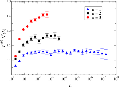
Figure 2: [Color online] Plot of $L^{-d/2}N^{-}(L)$, the average number of sites with negative excess at the termination of the algorithm scaled by the expected average $L^{d/2}$, vs. system size $L$, for $d=1,2,3$ samples with negative magnetization, in the $\Delta\rightarrow 0$ limit. The plot indicates convergence to a single value for the scaled variable in each dimension, consistent with $N^{-}\sim L^{d/2}$.

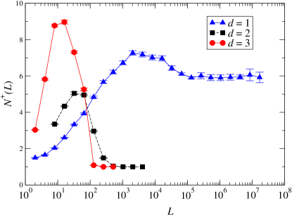
Figure 3: [Color online] Plot of $N^{+}(L)$, the number of remnant sites with positive excess in samples with positive magnetization, vs. $L$ for $d=1,2,3$, in the limit $\Delta\rightarrow 0$. The small numbers indicate that most of the positive excess is collected into less than 10 sites by the termination of the algorithm. The 1D data appear to converge to a constant $N^{+}(\infty)=5.96\pm 0.03$, while the 2D and 3D data apparently converge to $N^{+}(\infty)=1$

We also studied how densities of sinks and active sites converge to their final values $N^{-}L^{-d}$ and $N^{+}L^{-d}$. We have computed the number densities $\rho^{\pm}(n_{\mathrm{PR}},L)$ of the positive and negative sites as a function of “time” $n_{\mathrm{PR}}$ (number of PR cycles completed so far; $N_{\mathrm{PR}}=n_{\mathrm{PR}}$ at the end of the algorithm). The data, plotted for $d=2$ in Fig. 4, shows that the number density of sites with positive excess reaches a plateau consistent with constant $\rho^{+}=L^{-d}/2$ in the larger samples, i.e., $N^{+}\approx 1$ in samples with positive magnetization. In the late-time regime of few packets (that is, few active sites), the positive excess packets may move across the sample many times between global relabellings, in $d=2,3$. The density of negative excess sites decreases rapidly with the number of PR operations per site, though more slowly after the positive excess has coalesced.

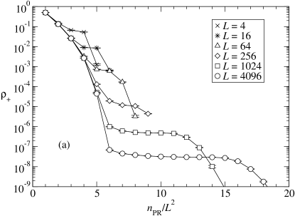
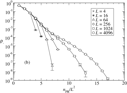
Figure 4: Plots of the number densities $\rho^{+}$ and $\rho^{-}$ vs. $n_{\mathrm{PR}}$, the number of PR steps executed during the algorithm for (a) positive excess packets (active sites) and (b) sinks, for $d=2$ FIFO, in the limit of small disorder. The density of positive sinks decreases very rapidly until, in the larger systems, a plateau $\rho^{+}=L^{-2}/2$ (i.e., an average of 1/2 of active site in the system, due to averaging over up-spin and down-spin ground states) is reached. One large collection of positive excess is moved around the system in samples with positive magnetization. This packet of excess annihilates broadly distributed sinks having a magnitude approximately proportional to $\Delta$. The density of negative-excess sites (sinks) decreases very rapidly, though the rate of decrease slows somewhat after the coalescence of positive excess into a single packet.

IV.3 Spatial structure of the remnant sinks

We can study the topography of the $u_{i}$ in the half of the ground states that have negative magnetization at small $\Delta$. One approach is to study the probability distribution and correlations of $u_{i}$ at all sites. We carry this out for $d=1$. Very closely related information can be found from the locations of the sites where $u_{i}=0$ at the termination of the algorithm. The spatial distribution of these remnant sinks reflects the history of the cancellation process. We have examined this spatial distribution in $d=1,2,3$. The terminal height field $u_{i}$ can also be computed from the final sink locations alone, when $\Delta\rightarrow 0$, so these two descriptions are closely related. One method to study the distribution of the sinks is to coarse-grain the distribution of the remnant sinks over a length $b$. The computed quantity we used, $N(b)$, is defined as the number of non-overlapping boxes of dimension $b^{d}$ that contain at least one sink. For a pure fractal, this would be used to estimate the box-counting dimension of the set. (One other characteristic of the final topography, which we study in Sec. V, is the geometry of paths along unsaturated bonds that start from sinks: these are the paths followed in global updates to identify reachable sites. At small disorder, these paths have trivial geometry.)

IV.3.1 Remnant sinks for $d=1$

After the terminal global update, the sites $i$ that are not sinks have a height label $u_{i}$ that equals the lattice distances to the nearest sink. Fig. 5 displays a plot of the scaled height probability distribution $L^{1/2}u^{1/2}P(u)$, where $P(u)$ is defined as the probability of a site $i$ to have a height $u$, for samples of various sizes $L$ at small $\Delta$. The plots show that $P(u)$ is well fit by a single power-law behavior, $P(u)\sim u^{-\tau}$, with $\tau=0.500\pm 0.005$. (This very small error bar in $\tau$ is estimated by finding the range of values which give a plateau to within statistical error for $P(u)L^{\tau}$, for $u>100$ and $2\,097\,152\geq L\geq 16\,384$ and assuming that the corrections to scaling are very small, so that deviations from a plateau represent only a statistical error in the exponent.)

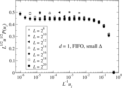
Figure 5: Plot of the scaled height distribution $L^{1/2}u^{1/2}P(u)$ vs. the sample-size normalized height, $L^{-1}u$, measured at the termination of the push-relabel algorithm for one-dimensional samples in the limit of weak disorder. The data collapse well to a constant, indicating that the distribution of heights behaves as $P(u)\sim u^{-1/2}$ from small scales up to heights $u\approx 10^{-2}L$, to within the numerical error bars. The error bars represent $1\sigma$ estimates for the sample-to-sample variation; the errors at a given $L$ are correlated, as the distribution at each scaled distance was computed from a single set of samples (the number of samples was at least $1700$ at each sample size). The global update frequency was set at $\Gamma=2L$.

We also characterized the sink distribution using $N(b)$. The estimates for this function are plotted in Fig. 6(a) for $d=1$. This data is also fit by a single power law, with $N(b)\sim b^{-D}$, where $D=0.500\pm 0.005$ (statistical error only). This estimate for the fractal dimension is consistent with $D=\frac{1}{2}$ for the set of remnant sinks in the small disorder limit.

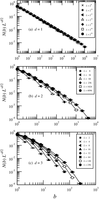
Figure 6: Plot of normalized box-counting data $N(b)L^{-d/2}$ vs. box size $b$ at $\Delta\rightarrow 0$. The quantity $N(b)$ counts the number of non-overlapping volumes of linear size $b$ that intersect the set of remnant sinks. The data shown here is averaged over samples for the auxiliary field configurations computed at the termination of the standard (non-blocking) push-relabel algorithm.

The result for fractal dimension $D$ and height-distribution exponent $\tau$ are related. In one dimension the distribution function $P(u_{i})$ is precisely related to the number $n_{s}(\ell_{ss})$ of sink-to-sink gaps of length $\ell_{ss}$ via

$$P(u_{i})=n_{s}(2u_{i}-1)+2\sum_{k=u_{i}}^{\infty}\left[n_{s}(2k)+n_{s}(2k+1)\right]\,.$$ (2)

In the continuum height limit, then, taking $\frac{dN(b)}{db}\sim n_{s}$ and $P\sim\int_{u_{i}}^{\infty}n_{s}(\ell_{ss})\,d\ell_{ss}$ gives $\tau=D$, consistent with our estimated values.

The structure of the sinks is very suggestive, when one considers the apparent relationship between the dynamics of the push-relabel algorithm in the limit of small-disorder and studies of the $A+B\rightarrow\emptyset$ reaction. In particular, Leyvraz and Redner studied the fractal structure of the $B$ particles in the limit that the $B$ particles are immobile. The primary difference between their analysis and this model is that the $A+B$ reaction was considered for diffusive $A$ particles. Here, the $A$ particles (corresponding to positive excesses) move directly towards the nearest $B$ particle (negative excess sites).

Our presumption will be that this distinction affects only the relationship between length scale and times. In the diffusive case, the time scale $t$ gives a length scale $\ell\sim t^{1/2}$. In the case of the push-relabel algorithm, we will take $t\sim\ell\ln(\ell)$ or, equivalently up to logarithms of logarithms, $\ell\sim t(\ln t)^{-1}$. This dependence comes from the linear “attraction” between the positive and negative excess sites, with a logarithmic correction reflecting the changes in direction that take place upon annihilation of positive and negative excess on successively larger scales, consistent with the finite-size scaling of the running times.

Given this correspondence, we expect the same domain structure of the negative excess sites in the final states as for the $B$ sites in the annihilation reaction with immobile $B$ particles. Leyvraz and Redner, using random walk arguments to sum up the densities of $A$ vs. $B$ particles, find the distribution of the distances $d_{BB}$ between neighboring $B$ sites to have the form $P(d_{BB})\sim d_{BB}^{-3/2}$. Identifying our $\ell_{ss}$ with $d_{BB}$ gives $\frac{dN(b=\ell_{ss})}{d\ell_{ss}}\sim n_{s}(\ell_{ss})\sim\ell_{ss}^{-3/2}$, which is numerically consistent with our statistics for the final configuration from the push-relabel algorithm. It is worthwhile to note that this type of picture is also in agreement with the structure of the 1D RFIM ground state reported by Schröder et al. Schröder et al. (2002), which was also derived using absorbing states of random walks. These connections support a unified picture of the dynamics of the push-relabel algorithm, the structure of the RFIM ground state, and the previously distinct study of annihilation reactions.

IV.3.2 Structure of remnant sinks, $d>1$

The results we obtain for small disorder in higher dimension are somewhat more complex. Scaling behavior is also seen, though the results can depend on the details of the algorithm. In the small disorder limit, the paths to the sinks are still linear, i.e., non-fractal and straight (the paths of course must be linear at all disorders when $d=1$). However, the fractal structure of the remnant sinks is more apparent in higher dimensions. In some cases there appears to be a new length scale, intermediate between the microscopic length and the sample size, that characterizes the final topography in samples with net negative magnetization.

The topography at the termination of the algorithm is displayed for $d=2$ in Fig. 7 for two variants of the PR algorithm. One variant is standard: pushes are executed without regard to the status of the destination site. We also consider in this section a “blocking” variant of the algorithm that forbids coalescence of positive excess. Whenever a push is attempted in the blocking version from a site $i$ with height $u_{i}$ to a site $j$ with $u_{j}=u_{i}-1$, the algorithm first checks whether the destination site already has positive excess. If there is positive excess at $j$, the algorithm does not push excess in that direction, but also does not relabel site $i$ (a relabel would be executed if there was no push due to saturated bonds with $r_{ij}=0$). This non-blocking variant slows down the algorithm some, but prevents the coalescence of the positive excess into a single packet. The number of positive excess sites does not decrease as quickly as in the non-blocking version, with the number of excess packets remaining comparable to the number of sinks, until $N^{+}$ or $N^{-}$ approach $L^{d/2}$. As can be seen in the figure, the sites with negative excess are clearly clustered on several scales for both variants of the algorithm.

(a)

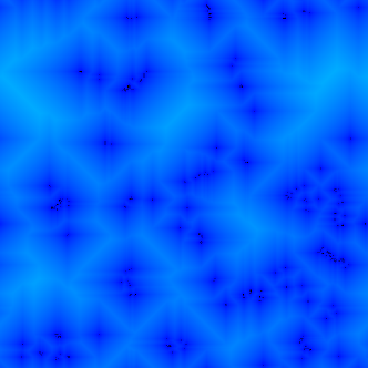
(b)

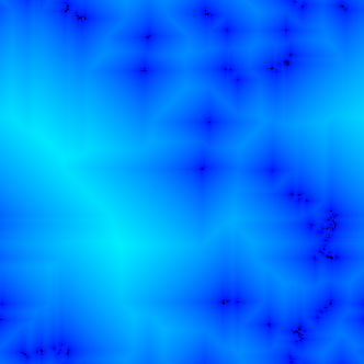
Figure 7: [Color online] Topography of the height field upon termination of the push-relabel algorithm, for a $d=2$ sample of linear size $L=512$, with weak disorder ($\Delta\rightarrow 0$ limit) for two different modifications of the push-relabel algorithm. The sample shown has negative magnetization. The lightness of the color (or grayscale) indicates the magnitude of the height field. Black pixels indicate spins with negative excess (height $u_{i}=0$), dark pixels indicate smaller heights, and light regions indicate higher heights. The height field and remnant sinks are shown for (a) the push-relabel algorithm with no limits on coalescence and (b) a modification where positive excess is not allowed to coalesce (the “blocking” version).

We studied this clustering for both variants by again applying box counting for the sites with negative excess. The box-counting data for the non-blocking variant, with $N(b)$ normalized by the number of sinks $N(0)\sim L^{d/2}$, is plotted as $L^{-d/2}N(b)$ vs. box size $b$ in Fig. 6(b,c). We examined this data for scaling behavior. The error bars are small enough that plotting the local exponent or slope of the $\ln$-$\ln$ plot was useful in studying the scaling. The scaling ansatz is that there is a crossover in the scale-dependent fractal dimension $D(b)$ at a scale $L^{X}$,

$$D(b)=\tilde{D}(bL^{-X})\,,$$ (3)

with $\tilde{D}(z)$ constant at small $z$ and crossing over to $\tilde{D}=d$ at large argument. The quantity used to estimate $D(b)$ is the discretized logarithmic derivative, $\delta\ln[N(b)]/\delta\ln(b)\equiv\left\{\ln[N(2^{1/2}b)]-\ln[N(2^{-1/2}b)]\right\}/\ln(2)$, whose negative gives an effective dimension when plotted as a function of $b$. The scaled plot of this estimate for $D(b)$ vs. $L^{-X}b$ is shown in Fig. 8, for our best fit values $X\approx 1.0$ ($d=1$), $X\approx 0.55$ ($d=2$) and $X\approx 0.5$ ($d=3$). Our estimates for the systematic error bars for $X$ are somewhat smaller for $d=1$ (less than 0.08) than for $d=2,3$, where variations in $X$ of the order of 0.12 provide plausible, but less clean, collapse to a single curve for $\tilde{D}$. The values of $D(b)$ or $\tilde{D}(b)$ at small argument provide an estimate for the effective box-counting dimension of the sinks at small scales. The $d=1$ data, as discussed in the previous section, give a fractal dimension consistent with $D=\frac{1}{2}$ at small scales. The $d=2$ data are consistent with a convergence to an effective dimension of $D\approx 0.4\pm 0.1$ over about 1 decade in scale at the smaller scales for the largest samples ($4096^{2}$) where the longest plateau in effective dimension is seen. The $d=3$ data are consistent with $D<0.2$ at small scales. At large scales, $b>L^{X}$, the data are quite consistent with $D=d$, i.e., a scale-independent density of sinks.

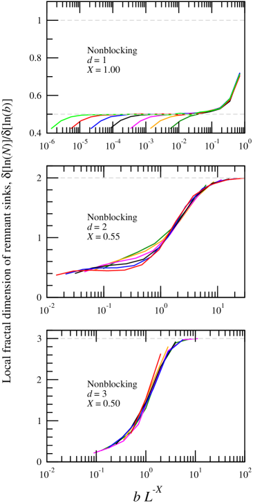
Figure 8: [Color online] Plot of the local dimension -$\frac{\delta[\ln(N)]}{\delta[\ln(b)]}$ of the set of remnant sinks plotted vs. scaled box size $bL^{-X}$. The data is sampled at the termination of the standard (non-blocking variant) push-relabel algorithm, for $d=1,2,3$. The sample sizes are $L=2^{8},2^{10},\ldots,2^{20}$ from the rightmost to the leftmost curves for $d=1$, $L=2^{7},2^{8},\ldots,2^{12}$ from the highest to the lowest curves for $d=2$, and $L=2^{3},2^{4},\ldots,2^{8}$ for $d=3$ (these curves overlap significantly). In the color version, the line colors run through the sequence dark green, orange, magenta, black, blue, red, light green, from smallest to largest $L$. The dashed light horizontal lines indicate local fractal dimension of $D=d$.

The logarithmic derivatives of the box-counting data for the blocking variant of FIFO in $d=2,3$ are displayed in Fig. 9. (For the case $d=1$, we find that while the number of active sites evolves differently, with the assumed form $N^{+}\sim L^{d/2}$ consistent with the data, the dimensions $D\approx 0.5$ and scaling $X\approx 1.0$ from the box-counting data are the same for the blocking and non-blocking variants.) The best collapses are seen for $X$ slightly less than 1, $X=0.93,0.90$ for $d=2,3$, respectively, with an estimated error of about 0.1. At small scales in $d=2$, the fractal dimension $D$ is approximately $0.9\pm 0.1$ at small scales. For $d=3$, the convergence is less clear, but is consistent with $D$ between 1.0 and 1.5 at small scales. Assuming a single fractal dimension over all scales, except for corrections near $b=L$, i.e., taking $X=1$, would give $D=d/2$, consistent with our data for the blocking variant.

Comparing the results for the distribution of sinks in these two variants of the algorithm and the density of packets discussed in Sec. IV.2 leads to a consistent qualitative picture for the interacting evolution of the active sites, sinks, and topography. In the non-blocking variant of the push-relabel algorithm, it appears that a scale is frozen in once the positive excess coalesces. The packet containing the positive excess moves all about the sample, cancelling each small negative excess site it encounters and changing directions to follow the height field $u_{i}$, until it is exhausted. This cancellation acts at small scales. The non-blocking variant, however, maintains roughly equal numbers of positive excess packets and negative excess sinks, so that the positive excess packets have a length scale that grows as the length scale of the sinks does, throughout the algorithm. The length scale for the topography of the height field is not set by the “freezing-out” of the positive excess into a single packet, then, but by the sample size. This leads to a scaling for the final distribution of sinks with $X\approx 1$, consistent within the large systematic error bars for $X$ in $d=2,3$. The non-blocking variant is more consistent in microscopic rules and with results for the annihilation dynamics of particles of constant charge.

Figure 9: [Color online] Plot of the local dimension $-\frac{\delta[\ln(N)]}{\delta[\ln(b)]}$ of the set of remnant sinks vs. scaled box size $bL^{-X}$ averaged over samples at the termination of the blocking variant of the push-relabel algorithm, for $d=2$ and $d=3$. The sample-size ranges are $L=2^{5}$, $2^{6}$, $\ldots$, $2^{12}$ for $d=2$ and $L=2^{1}$, $2^{2}$, $\ldots$, $2^{8}$ for $d=3$, with the leftmost curves corresponding to the largest samples. In the color version, the line colors run through the sequence dark green, orange, magenta, gray, blue, red, light green, black, from smallest to largest $L$. The error bars are determined by $1\sigma$ sample-to-sample fluctuations.

V General disorder and critical slowing down

We now consider larger values of $\Delta$, where the bonds can be saturated and block flow, making the rearrangements of excess more complicated than the $\Delta\rightarrow 0$ limit. We focus on the true transition at $\Delta=\Delta_{c}$ in $d=3$, but have also studied the topography of $u_{i}$ and timing for $\Delta\raisebox{-2.58334pt}{$\,\stackrel{{\scriptstyle\raisebox{-0.60275pt}{$\textstyle>$}}}{{\sim}}\,$}\Delta_{x}$ in $d=1,2$. Ogielski noted Ogielski (1986) that the PR algorithm takes more time to find the ground state near the transition in three dimensions from the ferromagnetic to paramagnetic phase. For the highest priority queue (HPQ) algorithm, identical to LPQ except that active sites with the highest height are kept at the front of the list, Middleton and Fisher Middleton and Fisher (2002); Middleton (2002a) studied this critical slowing down more extensively in the case of $d=3$ and work has also been carried out for $d=4$ Middleton (2002b). Here, we compare the scalings for the timing of FIFO and LPQ algorithms. The position of the peak in running time can itself be used to estimate $\Delta_{c}$, if one makes the natural assumption that the critical slowing down is greatest exactly at $\Delta_{c}$. This critical slowing down is certainly reminiscent of the slowing down seen in local algorithms for statistical mechanics at finite temperature, such as Metropolis, and even for cluster algorithms Swendsen and Wang (1987); Middleton (2004).

Critical slowing down results from the long length scales that arise near a continuous phase transition. To connect the topography of the $u_{i}$ to the physical system, we conjecture that the scale for the heights $u_{i}$ is given by the correlation length $\xi$. This assumption is natural: the maximal height in a domain of linear size $\xi$ must have a scale $\sim\xi$ for excess to be transported across a domain. The spin-spin correlation functions die off rapidly over longer ranges, so that the ground-state computation need not rearrange excess over scales greater than $\xi$. This conjectured relationship fits the numerical data well.

V.1 Timing for $d=1,2$

In one- and two-dimensional systems, there is a system-size-dependent crossover from large $\Delta$ to small $\Delta$ behavior. Above this crossover scale $\Delta_{x}(L)$, physical quantities such as correlation length and algorithmic quantities such as $N_{\mathrm{PR}}/n$ are expected to converge at large enough $L$ to an infinite-volume limit. This limit is expected to exhibit critical divergences with a critical point at $\Delta=0$.

Our unscaled data for the running time in $d=1$ and $d=2$ for FIFO are plotted in Fig. 10. From the known scaling for the correlation length $\xi\sim\Delta^{-2}$ Imry and keng Ma (1975); Nattermann and Villain (1988); Schröder et al. (2002) and taking $N_{\mathrm{PR}}/n\propto\xi\ln\xi$, one expects a straight line fit for $N_{\mathrm{PR}}/n$ when plotted vs. $\Delta^{-2}\ln\Delta$. We do not find convergence to a single exponent, but instead effective power law ranges from $N_{\mathrm{PR}}/n\sim(\Delta^{-2}\ln\Delta)^{0.25}$ to $N_{\mathrm{PR}}/n\sim(\Delta^{-2}\ln\Delta)^{0.7}$ over the range $\Delta=0.02$ to $\Delta=0.005$ for $L=2^{24}$. It may be that even larger samples are needed to see the expected divergence in $N_{\mathrm{PR}}$. Despite this, over the range $L=2^{14}\rightarrow 2^{24}$, we do find that the location of the peak in the running time is consistent with the scaling $\Delta_{x}\sim L^{-1/2}$. The peak in the running time per site therefore does occur when $\xi\sim L$.

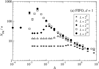
Figure 10: Running times for FIFO algorithm, (a) $d=1$ and (b) [color online] $d=2$ as a function of disorder $\Delta$ and normalized by sample volume. The error bars are small for $d=2$, so they are shown only for the largest size, where the error bars are largest.

A similar situation exists in $d=2$: the divergence of the running time with $\Delta$ is not fit well by the simplest scaling expectations. However, the location of the peak in the running time does scale in the expected fashion. The fitted location of the peak for the running time $L^{-2}N_{\mathrm{PR}}(\Delta)$ is plotted in Fig. 11. This data is quite consistent with $L\sim\ell_{0}\Delta^{-2y}e^{\Delta_{0}^{2}/\Delta^{-2}}$ G. Grinstein and Shang-keng Ma (1983), with best fit values $\ell_{0}=17\pm 4$, $\Delta_{0}^{2}=1.3\pm 0.2$, and $y=1.1\pm 0.2$, citing $2\sigma$-error bars and using all of the data points for $L\geq 16$. This error estimate is consistent with the variation that one gets by changing the fit to $L\geq 64$. The error bars are large enough that $y=1$ is certainly an acceptable value.

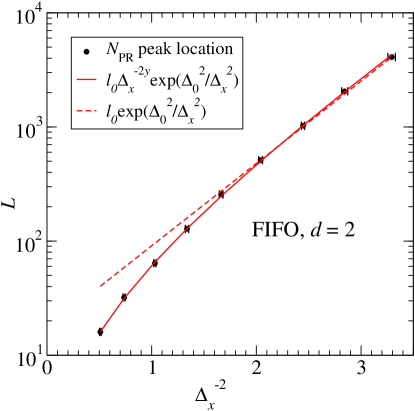
Figure 11: [Color online] A plot of the system size $L$ vs. $\Delta_{x}^{-2}$ (circles), where $\Delta_{x}$ is the fit to the locations of the peaks in $N_{\mathrm{PR}}$ displayed in Fig. 10. The dashed lines show a fit to the simplest expected form $L\sim\exp\left(-\Delta_{0}^{2}/\Delta_{x}\right)$ for $L\geq 256$ while the solid line is a fit to all data ($L\geq 16$) using the form $L\sim\Delta_{x}^{-2y}\exp(-\Delta_{0}^{2}/\Delta^{2})$, with best fit values $\ell_{0}=17.3$, $y=1.07$, and $\Delta_{0}^{2}=1.27$.

V.2 Topography for $d=1,2$

In contrast with the attempted scaling for the timing data, the topographical data for $d=1$ at larger $\Delta$ exhibit a clear scaling with the expected power-law behaviors. Fig. 12 presents an example of this scaling for the fraction $P_{1}(u,L,\Delta)$ of sites with height $u$ for $d=1$. The plot is of the scaled height distribution function $\Delta^{-1}u^{1/2}P_{1}(u,L,\Delta)$ vs. the height normalized by the correlation length, $u\Delta^{2}$, for various values of $L$ and $\Delta$. This plot assumes a correlation length $\xi(\Delta)\sim\Delta^{-2}$, with $\xi(\Delta)\ll L$, that $P(u)\sim u^{-1/2}$, as it is in the limit of small $\Delta$, and a properly normalized $P(u)$ ($\int du\,P(u)=1$), which together give a scaling form

$$P_{1}(u,L,\Delta)\sim\Delta u^{-1/2}\tilde{P}_{1}(u\Delta^{2})\,,$$ (4)

with $\tilde{P}(z)$ constant for small $z$. The data collapse very well for the range $1\gg\Delta\gg\Delta_{x}(L)$.

The data for $P_{2}(u)$ also exhibit scaling in $d=2$. The data then collapse well for disorders $\Delta\raisebox{-2.58334pt}{$\,\stackrel{{\scriptstyle\raisebox{-0.60275pt}{$\textstyle>$}}}{{\sim}}\,$}\Delta_{x}(L)$, if we choose a scale for the maximal $u$ that is proportional to $\Delta^{-2y}e^{-\left(\Delta_{0}/\Delta\right)^{2}}\propto\xi$, where we take the values of $y$ and $\Delta_{0}$ directly from the fit to the location of the peak in the timing. The scaled data shown in Fig. 13 are therefore in agreement with a scaling form

$$P_{2}(u,L,\Delta)\sim\xi^{-1}\tilde{P}_{2}(u/\xi)\,.$$

A fit assuming $\xi\sim e^{\Delta_{0}^{2}/\Delta^{2}}$ gave a somewhat worse scaling collapse.

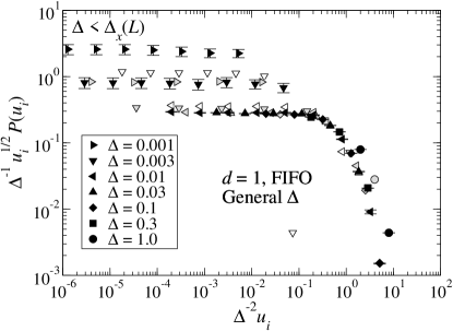
Figure 12: Scaling plot for the distribution of the heights at general $\Delta$ for $d=1$ and $L=2^{14},2^{18},$ and $2^{22}$, assuming the scaling form Eq. (4). The shape of the symbol indicates the value of $\Delta$, as indicated by the shape of the solid symbols in the legend. The color of the symbol indicates $L$, with white-filled symbols for $L=2^{14}$, gray-filled symbols for $L=2^{18}$, and black-filled symbols for $L=2^{22}$. The data for a broad range of $\Delta$, including those values that do not lie in the scaling range $1\gg\Delta\gg\Delta_{x}(L)$ and are therefore not expected to collapse, are shown. The points that do not collapse to the single curve are indicated by the region labeled $\Delta<\Delta_{x}(L)$ at the top of the graph. The points that do not fit for well to the right of the collapsed data are for $\Delta=1$, as indicated by the legend, where the correlation length is comparable to the lattice spacing. The data that are in the scaling range give a good collapse to a single curve, with many points overlapping to the extent that they are not visible. The scaling curve is flat over the range $10^{-4}<\Delta^{-2}u_{i}<10^{-1}$.

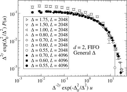
Figure 13: Scaling plot for the distribution $P(u_{i})$ of the final heights $u_{i}$ at general random-field strength $\Delta$ for $d=2$, with $L=2048$ and $L=4096$. The correlation length $\xi$ which sets the scale for the heights $u_{i}$ is taken to diverge as $\xi\sim\Delta^{-2y}\exp(\Delta_{0}^{2}/\Delta^{2})$, with the parameters $y=1.07$ and $\Delta_{0}=1.27$ taken from the scaling for the peak running time (Fig. 11). Curves and points that are expected to be outside of the scaling range are included for comparison. Besides small values of $u_{i}$ ($L=2048$ points near the top-center of the plot), the data that does not collapse is where$\Delta>1.25$, where $\xi$ is becoming comparable to the lattice size, and for $L=2048$, $\Delta=0.55$, which is on the low-$\Delta$ side of the running time peak (see Fig. 10). The curves over the range $0.55\leq\Delta\leq 1.00$ collapse relatively well; by the locations of the finite-size peaks in the running times of Fig. 10, this range of $\Delta$ corresponds to almost two decades in length scale: $64\leq L\leq 4096$. A fit to the simpler $\xi\sim\exp(\Delta_{0}^{2}/\Delta^{2})$ with a fit parameter $\Delta_{0}$ gives a worse scaling collapse.

V.3 Timing for $d=3$

Our data for the running time $N_{\mathrm{PR}}$ lend themselves well to scaling about the critical point. We have not attempted to separately infer the critical value $\Delta_{c}$ and the correlation length exponent $\nu$, which determine the correlation length $\xi$ via

$$\xi\sim|\Delta-\Delta_{c}|^{-\nu}\,,$$ (5)

but instead use the values determined in Ref. Middleton and Fisher (2002). These values, $\Delta_{c}=2.270(5)$ and $\nu=1.37(4)$ were found from scaling of the stiffness (energy change due to a change in boundary conditions) and spin-spin correlation functions and are consistent with, e.g., the location of the peak in the specific heat.

There is then one parameter to fit, the dynamic exponent $z$, which describes the divergence in the running time at $\Delta_{c}$, if one assumes the scaling

$$L^{-d}N_{\mathrm{PR}}\sim L^{z}w\left[\left(\Delta-\Delta_{c}\right)^{-1/\nu}L\right]$$ (6)

for the number of PR steps per site, where $w(x)\sim x^{-z}$ at large $x$ and $w(x)\sim|x|^{-z}\ln(|x|)$ as $x\rightarrow-\infty$, to be consistent with convergence to constant $L^{-d}N_{\mathrm{PR}}$ at $\Delta>\Delta_{c}$ and $L^{-d}N_{\mathrm{PR}}\sim\ln(L)$ for small $\Delta$ (note that the coefficient of this logarithm in the limit of large $L$ is probably different from what we find here, given that the true logarithmic behavior may not have been reached, as discussed in Sec. IV.1). Our best fits to this scaling form are plotted in Fig. 14 for the LPQ and FIFO data structures. Our estimates for the dynamic critical exponent $z$ are distinct for these two structures, with

$$z_{{\rm LPQ}}=0.93\pm 0.06;\,z_{{\rm FIFO}}=0.43\pm 0.06\,.$$ (7)

The error estimates reflect the range of fits that are consistent with a correction to scaling that is not too large; the statistical error bars are quite small for this data. The convergence for the FIFO data may be slower as the data diverge with $L$ more slowly, so that corrections to scaling arising from, for example, constants are more evident.

Given the scaling in the data about the thermodynamic critical point, it is natural to attempt to explain the critical slowing down as being due to the divergence of a correlation length $\xi$. The finite-size effect (scaling with $L$) then reflects how the running time diverges with $\xi$ in the infinite volume limit. The difference in the scaling of the running times for the two different data structures indicates different scaling with respect to $\xi$. This difference reflects the order in which the operations are carried out. For the LPQ algorithm, only a subset of the sites, those with the lowest $u_{i}$, are subject to PR operations. This is in contrast with FIFO, where all active sites are considered cyclically. The FIFO structure leads to a more rapid coalescence of active sites and cancellation of positive packets with sinks. It appears that it then takes fewer PR operations to transport the same quantity of excess across a domain as the domain size increases. In the LPQ implementation, the value $z\approx 1.0$ suggests that order $\xi$ operations are carried out on average in domains of size $\xi^{d}$ (note that $z\approx 1.0$ in 3D for highest priority queues ).Middleton and Fisher (2002); Middleton (2002b). This is consistent with each site being relabeled an average of a multiple of $\xi$ times. The LPQ algorithm coalesces the positive excess by sweeping across the height. The FIFO algorithm must relabel the sites in such a way that only a small fraction of the sites are relabeled to height $u_{i}\sim\xi$, with $P(u)\sim u^{z-2}$ if $P(u)$ is described by a simple power law and the number of relabels is proportional to $N_{\mathrm{PR}}$. Nonetheless, taking $\xi$ as a cutoff for the distribution of $u_{i}$ in FIFO is consistent with the assumption that some portion of the excess must be rearranged across the width of a domain.

We note that there are many distinct scaling plots that can be made from the timing data. The running times for positively magnetized and negatively magnetized samples differs significantly for small $\Delta$, due to the asymmetry between the negative excess sinks and the positive excess packets at active sites. For large $\Delta$, the algorithm regains its symmetry, in that the average magnetization is near zero and any sample is a nearly even mix of up-spin and down-spin domains. One of the plots that we found to be a sensitive test of scaling was to compare the running time $N_{\mathrm{PR}}$ between samples with opposite magnetizations. In particular, the relative rms fluctuations $\sigma_{N_{\mathrm{PR}}}^{+}$and $\sigma_{N_{\mathrm{PR}}}^{-}$ in the operation count for samples with positive and negative magnetization, respectively, vary in a rapid fashion near criticality. The dimensionless ratio $R_{+-}=\sigma_{N_{\mathrm{PR}}}^{+}/\sigma_{N_{\mathrm{PR}}}^{-}$ is a non-monotonic function characterizing the distribution of running times. This function of $\Delta$ and $L$ collapses very well for $L\raisebox{-2.58334pt}{$\,\stackrel{{\scriptstyle\raisebox{-0.60275pt}{$\textstyle>$}}}{{\sim}}\,$}16$ with no adjustable parameters (taking $\Delta_{c}$ and $\nu$ fixed as stated earlier). A plot of this collapse is shown in Fig. 15 for the FIFO algorithm. The parameter-free fit (subject to using published values for $\Delta_{c}$ and $\nu$) provides a clear confirmation of scaling for the distribution of running times.

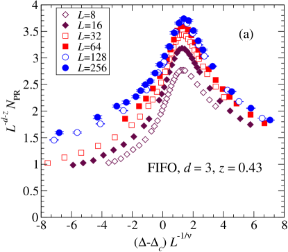
Figure 14: [Color online] Plot of scaled running time in $d=3$ for (a) the FIFO data structure, with a fit value of $z=0.43$, and (b) the LPQ data structure, with dynamic exponent $z=0.93$. The scaling fit assumes $\Delta_{c}=2.270$ and $\nu=1.37$ as fixed parameters.

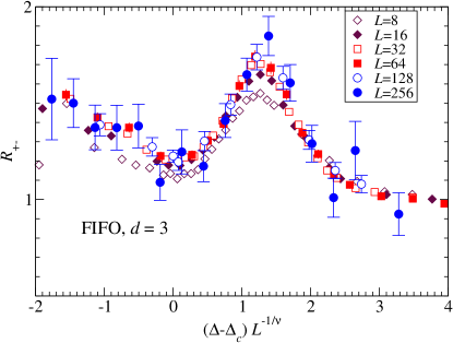
Figure 15: [Color online] Plot of the dimensionless ratio $R_{+-}$ of the rms fluctuations $\sigma_{N_{\mathrm{PR}}}^{+}$ in $N_{\mathrm{PR}}$ (time to find the ground state) positive magnetization samples to the corresponding quantity $\sigma_{N_{\mathrm{PR}}}^{-}$ in negative magnetization samples plotted vs. the scaled disorder $(\Delta-\Delta_{c})L^{1/\nu}$, for samples of sizes $L=8$, 16, 32, 64, 128, and 256. The values $\Delta_{c}=2.270$ and $\nu=1.37$ were assumed, based on scaling of physical (not algorithmic) quantities, so this parameter-free fit is a direct check of scaling for the distributions of running times.

V.4 Topography at $\Delta=\Delta_{c}$ for $d=3$

The evolution of the auxiliary fields are closely connected with the timing of the algorithm, as seen in Sec. IV for $\Delta\rightarrow 0$. We have studied the final topography of the height field and the paths that lead to the sinks for $d=3$ and general $\Delta$. We use this information to study the characteristic topography at $\Delta$ near $\Delta_{c}$ when using the FIFO data structure.

A study of the box-counting data for the sinks gives less information than for $\Delta=0$. For any $\Delta<\Delta_{c}$, there will be a finite density of minority spins (spins opposite to the net magnetization). This density drops very rapidly in $d=3$ as $\Delta$ decreases below $\Delta_{c}$, but these minority spins result in a fractal dimension of $D=3$ at all scales $\ell$ greater than the typical separation between the minority spins. We found no obvious singularity in $N(b)$ for $\Delta\approx\Delta_{c}$: the logarithmic derivative for $N(b)$ converges rapidly to $\approx 3.0$ for $b>8$, for the disorder range $2\leq\Delta\leq 3$ . The spatial distribution of the sinks is non-fractal for $\Delta\approx\Delta_{c}$ (at least from simplest the box-counting perspective; there will of course be some singularities in the density and correlations of down spins at $\Delta_{c}$).

A feature of the topography that is much more sensitive to the phase transition is the distribution of the $u$. The height values $u_{i}$ reflect long range correlations of the spins (minority sinks give $D=3$ but are localized in their effect on the $u_{i}$). In Fig. 16, we compare the distributions $P(u)$ for the two largest systems we studied at finite $\Delta$, $L=128$ and $L=256$ to indicate how $L$ and $\Delta$ appear to affect the height distributions. At large $\Delta$, the height distribution decreases exponentially with $\Delta$, $P(u)\sim e^{-u/\xi(\Delta)}$. This is consistent with spin-spin correlations decreasing exponentially over a characteristic length scale $\xi(\Delta)$ in the paramagnetic phase. For $\Delta$ significantly above $\Delta_{c}$, the $P(u)$ are relatively independent of $L$. For $\Delta\ll\Delta_{c}$, the height distribution peaks at a scale $u_{i}^{p}\sim L^{X}$ that grows with system size. This is consistent with the data of Fig. 8, which gives a crossover in the spatial distribution of the sinks (for the non-blocking variant). Above this length scale $\sim L^{0.5}$, the distribution of sinks becomes uniform, leading to a cutoff in the $u_{i}$, or distance to the nearest sink, above that scale. Near criticality, the distribution $P(u)$ must crossover between these two behaviors, one decreasing at small $u$ and the other increasing. The distribution changes rapidly with $\Delta$ and $L$ in this region. We find that the critical distribution is not varying exponentially rapidly for some $\Delta\approx\Delta_{c}$.

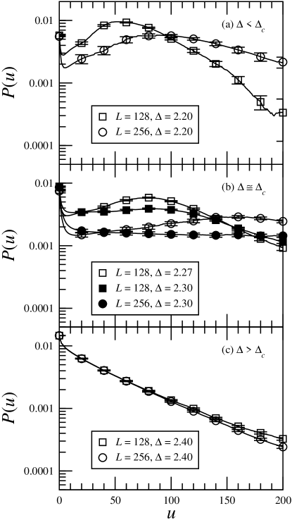
Figure 16: Plot of the height probability distribution $P(u)$ for different values of disorder $\Delta$ and size $L$, for $d=3$ near the critical value $\Delta_{c}=2.27$. The symbols and error bars are for a sampling of points; the solid lines are measured for every integer value of $u$. (a) At low $\Delta<\Delta_{c}$, the distribution of heights $u$ has a peak at an $L$-dependent scale. (b) Near $\Delta_{c}$, the distribution of $u$ is much less dependent on $u$ and is nearly constant over a large range of $u$ (on this scale, power laws are nearly constant), though the form of $P(u)$ varies rapidly for $\Delta\approx\Delta_{c}$. (c)High $\Delta$values, here $\Delta=2.40>\Delta_{c}$ give a distribution $P(u)\sim e^{-u/\xi}$.

One other feature of the topography that we have investigated is the structure of the paths that connect down-spin sites to a sink at the final step of the algorithm. When $\Delta$ is small, these paths must be linear, as there are no saturated bonds. Near criticality, many bonds are saturated and there is the potential that the paths to a sink could be rather torturous, as they would need to avoid saturated links. Numerical studies were carried out to measure the paths to the sinks. When carrying out a global update, we maintain a destination label that gives the location of the sink to which any positive excess will flow. For fixed height of each site with $u<\infty$, the Euclidean distance $r$ of that site to the sink given by the destination label is computed. The FIFO data can be used to estimate a fractal dimension $d_{f}$, $u\sim r^{d_{f}}$, for the paths which guide the pushing of the excess. Near $\Delta_{c}$, it appears that the paths are nearly linear. For $u>10$ and $\Delta\leq 2.30$, the Euclidean distance $r$ was linear in height $u$, with an effective fractal exponent in the range $0.9<d_{f}<1.1$ for samples of size $L=256$.

VI Summary

In this paper, we have studied the dynamics of the auxiliary fields used in the push-relabel algorithm to find the exact ground state of the random-field Ising magnet, a prototypical glassy model. These dynamics, and the final state of the fields found during the solution, reflect both the underlying physical model and the special dynamics of the algorithm. There is some freedom of choice for these dynamics: we studied primarily the FIFO queue with global updates, which is the fastest algorithm we have used and is also most directly similar to the synchronous evolution used to model physical dynamics. The evolution of the auxiliary fields is roughly a rearrangement and cancellation of the locally varying external fields. The extent of this cancellation determines the size of the domains in the RFIM ground state.

In the limit of small disorder, the dynamics of the field of excesses is that of a potential-driven annihilation reaction, $A+B\rightarrow\emptyset$. The algorithmic time per spin to find the ground state for $N$ spins is apparently linear in $\ln(N)$, though a simple logarithmic behavior is seen only at large system sizes. The densities of the mobile positive excess fields (active sites) and the immobile negative excess fields (sinks) decreases very rapidly with time. When the positive excess is allowed to coalesce, the number of positive sites becomes of order unity before the ground state is found. This coalescence leads to a cutoff in length scale $L^{X}$ in a sample of linear size $L$ that limits the range of scales over which the sinks at the end of the algorithm can be described as fractal. If coalescence is forbidden, the remnant sinks appear be described by a fractal measure all the way up to scale that is nearly equal to $L$. The fractal dimension in $d=1$, $D\approx 0.50$, is consistent with random walk arguments that have been developed for diffusive annihilation-reaction dynamics F. Leyvraz and S. Redner (1992). For $d=2$, $D\approx 0.4$ and the fractal dimension $D<0.2$ for $d=3$.

Diverging length scales in the RFIM influence the running time for the algorithm at general disorder values. While the running time itself is not easily scaled, the peak location for $d=1,2$, $\Delta_{x}(L)$, scales as expected from calculations for the divergence of the correlation length $\xi$ with $\Delta$ in the RFIM Imry and Ma (1975); Binder (1983); Grinstein and Ma (1982). In particular, for $d=2$, the location of the peak in the running time for a finite system and the distribution of the height fields near the transition give evidence for the predicted form for the power law corrections to the exponential dependence of $\xi$ on $\Delta^{-2}$. Further examination of the data may be useful in explaining how $N_{\mathrm{PR}}(\Delta)$ diverges. In $d=3$, the scaling of the running time (and its distributions, as seen in Fig. 15) are quite consistent with values Middleton and Fisher (2002) for the critical value $\Delta_{c}$ and correlation length exponent $\nu$ obtained from simulations for the physical properties of the RFIM. For $\Delta\approx\Delta_{c}$ in $d=3$, the distribution of the field corresponding to the potential $u_{i}$ generated by the sinks is nearly constant in $u_{i}$. For small $\Delta>\Delta_{x}$, $P(u_{i})\propto u_{i}^{-1/2}$ for $u\ll\xi$ in $d=1$ and varies very slowly for $u_{i}$ up to $\xi$ in $d=2$.

We believe that these consistent and strong connections between algorithm dynamics, the physics of the RFIM, and the mathematics used to describe annihilation processes provide insight into both the push-relabel algorithm and the RFIM. One is tempted to speculate that relating the rearrangement of fields in the push-relabel algorithm to finding the domains in the RFIM might help in analytic approaches, either in finite dimensions or on hierarchical lattices M. S. Cao and J. Machta (1993). The running time of the PR algorithm is directly related to the average of the potential or height field; distinct algorithms give different scaling for this average, though the physical ground state that is found is identical. A better understanding of this dynamical exponent $z$ given by the average height, is likely to shed light on both the algorithm and the RFIM ground state at criticality.