The Kondo lattice model introduced in 1977 describes a lattice of localized magnetic moments interacting with a sea of conduction electrons. It is one of the most important canonical models in the study of a class of rare earth compounds, called heavy fermion systems, and as such has been studied intensively by a wide variety of techniques for more than a quarter of a century. This review focuses on the one dimensional case at partial band filling, in which the number of conduction electrons is less than the number of localized moments. The theoretical understanding, based on the bosonized solution, of the conventional Kondo lattice model is presented in great detail. This review divides naturally into two parts, the first relating to the description of the formalism, and the second to its application. After an all-inclusive description of the bosonization technique, the bosonized form of the Kondo lattice hamiltonian is constructed in detail. Next the double-exchange ordering, Kondo singlet formation, the RKKY interaction and spin polaron formation are described comprehensively. An in-depth analysis of the phase diagram follows, with special emphasis on the destruction of the ferromagnetic phase by spin-flip disorder scattering, and of recent numerical results. The results are shown to hold for both antiferromagnetic and ferromagnetic Kondo lattice. The general exposition is pedagogic in tone.

Chapter 0 An Introduction to the Kondo Lattice

The Kondo lattice is one of the most important canonical models used to study strongly correlated electron systems, and has been the subject of intensive study. Other canonical models for strongly correlated systems include the Hubbard model, which is discussed in section 2, and the periodic Anderson model, which is introduced in section 2 . The Kondo lattice describes the interaction between a conduction band, containing Bloch-like delocalized electrons, and a lattice of localized magnetic moments. Its importance is due both to its relevance to several broad classes of real materials, and to the the fundamental theoretical challenge it presents; methods developed for the Kondo lattice are expected to aid in formulating methods for other strongly correlated electron systems. Hereafter, follows a description of the Kondo lattice, and in particular the 1D Kondo lattice at partial band filling.

This chapter provides a general introduction to the Kondo lattice model. The chapter is organized as follows: In section 1 the Kondo lattice is derived as a special case of a general two-band electron system. This serves to provide both a definition of the Kondo lattice model, and to provide a clear statement of the assumptions required to derive the model; the main assumption is that the Wannier states for one of the bands are atomic-like. Applications of the Kondo lattice to real materials are discussed in section 2. The description of manganese oxide perovskites follows in straightforward fashion from the derivation of section 1, and is discussed in section 1. Section 2 considers the Kondo lattice description of rare earth and actinide compounds. The application in this case is indirect, and requires the derivation of the Kondo lattice from the more fundamental periodic Anderson model.

1 Derivation of the Kondo lattice model

The Kondo lattice is a special case of a general two-band electron system with interband interactions: The Kondo lattice specializes to the case in which the electrons in one of the bands remain localized at their lattice sites. In this section the Kondo lattice model is derived from a general two-band system with standard electron-electron interactions. The derivation serves two purposes. Firstly it defines the conventional Kondo lattice model, which in its 1D form will be the primary focus of chapters 4 and 5. Secondly, the derivation permits a clear statement of the assumptions required to derive the Kondo lattice from a general two-band system. This helps to identify the types of real materials which may be modelled by the Kondo lattice. The applications to real materials are discussed in section 2.

The starting point is a two-band electron system with band indices $c$ and $f$. $c$ labels the conduction band, and $f$ labels the band of localized electrons; the $f$ is to suggest the localized $f$-electrons in rare earth and actinide compounds. In the simplest case, both $c$ and $f$ bands are assumed to have spin degeneracy only. (This point is discussed further in section 2.) The electron-electron interaction energy between two electrons at $x$ and $x^{\prime}$ is given by $V_{\sigma,\sigma^{\prime}}(x-x^{\prime})$, as discussed in section 13.B. The interaction is usually spin-isotropic, $V_{\sigma,\sigma^{\prime}}(x-x^{\prime})=V(x-x^{\prime})$, and in this case represents Coulomb repulsion between the electrons. Since attention has been directed toward the spin-anisotropic Kondo lattice (Shibata, Ishii and Ueda 1995, Zachar, Kivelson and Emery 1996, Novais, it et al. 2002a,2002b), the Kondo lattice model will be derived here for general spin interactions. The total energy from electron-electron interactions in a lattice with two bands is given by

$$V=\frac{1}{2}\sum_{n_{1},\ldots,n_{4}}\sum_{j_{1},\ldots,j_{4}}\sum_{\sigma,\sigma^{\prime}}V_{\sigma,\sigma^{\prime}}(n_{1}j_{1},\ldots,n_{4}j_{4})c^{\dagger}_{n_{1}j_{1}\sigma}c^{\dagger}_{n_{2}j_{2}\sigma^{\prime}}c_{n_{3}j_{3}\sigma^{\prime}}c_{n_{4}j_{4}\sigma}$$ (1)

where $n_{i}=c,f$ labels the band and the $j_{i}$’s labels the lattice site. This is a straightforward generalization of the single-band electron-electron interaction introduced in section 13.B. From Eq. (10), the matrix element in Eq. (1) is given by

$$V_{\sigma,\sigma^{\prime}}(n_{1}j_{1},\ldots,n_{4}j_{4})=\int_{L}dx\int_{L}dx^{\prime}\,V_{\sigma,\sigma^{\prime}}(x-x^{\prime})$$

$$\times \Phi^{*}_{n_{1}\sigma}(x-j_{1}a)\Phi^{*}_{n_{2}\sigma^{\prime}}(x^{\prime}-j_{2}a)\Phi_{n_{3}\sigma^{\prime}}(x^{\prime}-j_{3}a)\Phi_{n_{4}\sigma}(x-j_{4}a)$$

in 1D, where $\Phi_{n\sigma}(x-ja)$ is the wavefunction for the Wannier state $|nj\sigma\rangle$ as in Eq. (11). The generalization to higher dimensions is straightforward.

The Kondo lattice interaction $V_{\mbox{\scriptsize{KL}}}$ may be derived from the full electron-electron interaction Eq. (1) under the following assumptions, listed in order of importance: i) There is exactly one localized $f$-electron at each lattice site $j$. The set of lattice sites occupied by $f$-electrons is generally taken to be the entire lattice for the Kondo lattice model, but may be a small fraction of all lattice sites (modelling dilute Kondo impurities), and may even be a single lattice site (the original single impurity Kondo model ). If this is the case, then the label $j$ in the Kondo lattice interaction (cf. Eq. (10) below) refers only to those lattice sites containing an $f$-electron. ii) The matrix elements $V_{\sigma,\sigma^{\prime}}(n_{1}j_{1},\ldots,n_{4}j_{4})$ of Eq. (LABEL:4.2) are assumed to be negligible, unless $j_{1}=j_{2}=j_{3}=j_{4}$. Thus only on-site interactions are considered, similar to the Hubbard model interaction. iii) Electron-electron interactions between electrons in the same band may be neglected. These three assumptions reduce the full electron-electron interaction of Eq. (1) to on-site interactions between conduction electrons and $f$-electrons. Moreover, the interactions preserve the number of $f$-electrons at each site. The motivation for making assumptions ii) and iii) is mainly to distil the problem into the simplest form, but without losing the essential physics. Assumption iii), neglecting intraband interactions, is made so as to focus on the interband interactions of central interest, and is often relaxed. On-site conduction electron-conduction electron interactions are considered for the 1D Kondo lattice in section 2, and do not qualitatively alter the interband interactions. As for interactions between the localized electrons, note that on-site interactions are prohibited by assumption i). Nearest-neighbour interactions between the localized electrons in the 1D Kondo lattice are occasionally considered (White and Affleck 1996). Indeed in real systems there will exist dipolar and exchange interactions between the localized electrons, as in the 1D Kondo lattice compound Cu(pc)I (Ogawa, et al. 1987). However, since for the Kondo lattice these interactions are nearest-neighbour, they will in general be far weaker than the on-site interactions . A similar argument applies to nearest-neighbour conduction electron-conduction electron and conduction electron-localized electron interactions. This argument, which is identical to that made in the Hubbard model (cf. section 13.B and see Hubbard (1963)), is the motivation for assumption iii). Assumption i) is the main assumption in the Kondo lattice, and distinguishes it from general two-band systems. The two-band materials for which assumption i) holds will be discussed in section 2.

It is straightforward to verify that under assumptions i) - iii), Eq. (1) reduces to

$$V_{\mbox{\scriptsize{KL}}} = V_{\rm dir}+V_{\rm ex}\,,$$

$$V_{\rm dir} = \sum_{j,\sigma,\sigma^{\prime}}V^{\rm dir}_{\sigma,\sigma^{\prime}}\,c^{\dagger}_{cj\sigma}c_{cj\sigma}n_{fj\sigma^{\prime}}\,,\quad V^{\rm dir}_{\sigma,\sigma^{\prime}}=V_{\sigma,\sigma^{\prime}}(f0,c0,c0,f0)\,,$$

$$V_{\rm ex} = -\sum_{j,\sigma,\sigma^{\prime}}V^{\rm ex}_{\sigma,\sigma^{\prime}}\,c^{\dagger}_{cj\sigma}c_{cj\sigma^{\prime}}c^{\dagger}_{fj\sigma^{\prime}}c_{fj\sigma}\,,\quad V^{\rm ex}_{\sigma,\sigma^{\prime}}=V_{\sigma,\sigma^{\prime}}(f0,c0,f0,c0)\,.$$ (3)

In Eq. (3), $n_{fj\sigma}=c^{\dagger}_{fj\sigma}c_{fj\sigma}$ is the $f$-electron number operator, and the matrix elements at right follow the notation of Eq. (LABEL:4.2).

The Kondo lattice interaction $V_{\mbox{\scriptsize{KL}}}$ may be written in conventional form by introducing pseudo-spin operators for the $f$-electrons: Since the $f$-electrons are confined to their lattice sites, the only degree of freedom available to the $f$-electrons is spin. Define the $f$-electron spin operator ${\bf S}_{j}=(S_{j}^{x},S_{j}^{y},S_{j}^{z})$ by

$$S^{x}_{j} = \frac{1}{2}\left(S^{+}_{j}+S^{-}_{j}\right)\,,$$

$$S^{y}_{j} = \frac{1}{2i}\left(S^{+}_{j}-S^{-}_{j}\right)\,,$$

$$S^{z}_{j} = \frac{1}{2}\left(n_{fj\uparrow}-n_{fj\downarrow}\right)\,.$$ (4)

The spin raising and lowering operators are defined by

$$S^{+}_{j}=c^{\dagger}_{fj\uparrow}c_{fj\downarrow}\,,\quad S^{-}_{j}=c^{\dagger}_{fj\downarrow}c_{fj\uparrow}\,.$$ (5)

A little algebra establishes the usual spin commutation relations for the Cartesian components of ${\bf S}_{j}$:

$$\left[S^{\alpha}_{j},S^{\beta}_{j^{\prime}}\right]=i\,\delta_{j,j^{\prime}}\,\epsilon_{\alpha\beta\gamma}\,S^{\gamma}_{j}\,,$$ (6)

where $\alpha,\beta,\gamma=x,y,z,$ and where $\epsilon_{\alpha\beta\gamma}$ is the third rank totally antisymmetric unit tensor. Using the localized spin operators, the Kondo lattice interaction $V_{\mbox{\scriptsize{KL}}}$ of Eq. (3) may be written in the form

$$V_{\mbox{\scriptsize{KL}}}=\frac{J_{\parallel}}{2}\sum_{j}\left(n_{cj\uparrow}-n_{cj\downarrow}\right)S^{z}_{j}+\frac{J_{\perp}}{2}\sum_{j}\left(c^{\dagger}_{cj\downarrow}c_{cj\uparrow}S^{+}_{j}+{\rm h.c.}\right)$$ (7)

to an additive constant depending on the dispersion of the conduction electrons, where $n_{fj\sigma}=c^{\dagger}_{fj\sigma}c_{fj\sigma}$ the $c$-electron number operator. The interaction parameters in Eq. (7) are given by

$$J_{\parallel} = 2\left(V^{\rm dir}_{\parallel}-V^{\rm dir}_{\perp}-V^{\rm ex}_{\parallel}\right)\,,$$

$$J_{\perp} = -2V^{\rm ex}_{\perp}\,$$ (8)

where the direct and exchange integrals of Eq. (3) have been decomposed into spin-parallel and spin-perpendicular components following Eq. (7):

$$V^{\rm dir}_{\sigma,\sigma^{\prime}} = V^{\rm dir}_{\parallel}\delta_{\sigma,\sigma^{\prime}}+V^{\rm dir}_{\perp}\delta_{\sigma,-\sigma^{\prime}}\,,$$

$$V^{\rm ex}_{\sigma,\sigma^{\prime}} = V^{\rm ex}_{\parallel}\delta_{\sigma,\sigma^{\prime}}+V^{\rm ex}_{\perp}\delta_{\sigma,-\sigma^{\prime}}\,.$$ (9)

Note that $J_{\parallel}\neq J_{\perp}$ for a general spin-anisotropic interaction. For a spin-isotropic interaction, $V_{\sigma,\sigma^{\prime}}(x-x^{\prime})=V(x-x^{\prime})$, the direct interaction between the conduction electrons and the $f$-electrons drops out of the problem, and the Kondo lattice interaction takes its conventional form

$$V_{\mbox{\scriptsize{KL}}}=J\sum_{j}{\bf S}_{cj}{\bf\cdot}{\bf S}_{j}\,,\quad\quad J=J_{\parallel}=J_{\perp}\,,$$ (10)

where ${\bf S}_{cj}$ are pseudo-spin operators for the conduction electrons, defined as in Eqs. (4) and (5) for the $f$-electrons. Eq. (10) represents a Heisenberg-type interaction between an $f$-electron, and the conduction electron spin at the same site. The interaction parameter in the spin-isotropic case is given by the exchange integral

$$J=-2V^{\rm ex}=2\int_{L}dx\int_{L}dx^{\prime}\,V(x-x^{\prime})\Phi^{*}_{f}(x)\Phi^{*}_{c}(x^{\prime})\Phi_{f}(x^{\prime})\Phi_{c}(x)\,,$$ (11)

where $\Phi_{n}(x)$ is the Wannier wavefunction Eq. (11) at $j=0$ without the Pauli spinor.

The full Kondo lattice hamiltonian $H_{\mbox{\scriptsize{KL}}}$ is obtained by adding the kinetic energy to the interaction $V_{\mbox{\scriptsize{KL}}}$. Since the $f$-electrons are fixed at their lattice sites, the kinetic energy of the $f$-band is constant, and may be neglected. The full hamiltonian for the Kondo lattice then consists of $V_{\mbox{\scriptsize{KL}}}$, together with the conduction electron kinetic energy. In the simplest case, the conduction electrons hop between nearest-neighbour sites $\langle ij\rangle$ only, as discussed in section 13.A (cf. Eq. (5) for 1D). The hamiltonian for the Kondo lattice is then

$$H_{\mbox{\scriptsize{KL}}}=-t\sum_{\langle ij\rangle}\sum_{\sigma}c^{\dagger}_{ci\sigma}c_{cj\sigma}+J\sum_{j}{\bf S}_{cj}{\bf\cdot}{\bf S}_{j}\,,$$ (12)

for a spin-isotropic interaction. $H_{\mbox{\scriptsize{KL}}}$ is the conventional Kondo lattice hamiltonian. It is straightforward to extend $H_{\mbox{\scriptsize{KL}}}$ to include next-nearest-neighbour hopping, and so on, and spin-anisotropic interactions may be included by using Eq. (7) for $V_{\mbox{\scriptsize{KL}}}$ (see eg, Shibata, Ishii and Ueda (1995), Zachar, Kivelson and Emery (1996), Novais, it et al. (2002a,2002b)). While some of these (and other) variants of the Kondo lattice will be discussed at various stages later, the conventional Kondo lattice (in 1D) will be the main focus of this review. Unless otherwise noted, Eq. (12) defines the Kondo lattice model as discussed here.

The Kondo lattice model contains two parameters. The first is the coupling $J$ (or the dimensionless parameter $J/t$). Both large and small values of $|J|/t$ are physically relevant, as will be discussed immediately below in section 2. For large values the relevant sign of $J$ is negative, and this is called a ferromagnetic coupling since it favours an alignment of the conduction electron spin with the spin of the localized $f$-electron. For small values of $|J|/t$ the relevant sign of $J$ is positive, and this is called an antiferromagnetic coupling since it favours an opposite alignment of the conduction electron spin with the spin of the localized $f$-electron. The second parameter in the Kondo lattice is the number of conduction electrons. This is measured by the filling $n=N_{e}/N$, where $N_{e}$ is the number of conduction electrons and $N$ is the number of lattice sites. $N$ coincides with the number of $f$-electrons. A half-filled conduction band corresponds to $n=1$, and $n<1$ is called a partially-filled band. It is usual to consider only fillings in the range $0<n\leq 1$ in the Kondo lattice, and attention is restricted to this range.

2 Relevance of the Kondo lattice to real materials

The Kondo lattice describes materials in which the predominant interactions are between two distinct varieties of electrons; localized electrons possessed of a magnetic moment, and itinerant conduction electrons. The two varieties are described in the derivation of the previous section with the band indices $f$ and $c$, respectively. This situation is realised in two broad and important classes of materials: (i) Manganese oxide perovskites, in which there generally exists a mixture of ${\rm Mn}^{3+}$ and ${\rm Mn}^{4+}$ ions. (ii) Rare earth and actinide compounds, broadly classed as heavy fermion materials, in which atomic-like $f$-electrons interact with a conduction band. The Kondo lattice description of these materials is discussed in sections 1 and 2, respectively. Before proceeding, however, it is useful to give a brief discussion of what the Kondo lattice model does not describe.

In using the Kondo lattice to model real materials, first note that as an electron system the Kondo lattice model neglects electron-phonon coupling; it ignores interactions between the electrons and the vibrations of the underlying lattice of ions. This may result in the Kondo lattice model being unable to reproduce important properties of real materials. For example, Millis, Littlewood and Shraiman (1995) have argued that this is indeed the case in the manganese oxide perovskites. The Kondo lattice is often used to model this class of materials (cf. section 1 below). Millis, et al. (1995) argue that the predictions of the Kondo lattice disagree with the experimental data by an order of magnitude or more. They propose that the discrepancy arises from the neglect of strong electron-phonon coupling coming from a Jahn-Teller splitting of the ${\rm Mn}^{3+}$ ion. If this is true (and the issue is not yet settled), then an electron-phonon interaction term must be added to $H_{\mbox{\scriptsize{KL}}}$ .

A second point to note is that the Kondo lattice model Eq. (12) allows only two degrees of freedom for each band; either spin up or spin down. In the materials described by the Kondo lattice there is further degeneracy: In the manganese oxides, the localized electrons are three Hund’s rule coupled $d$-band electrons, and the localized band carries spin 3/2. In the heavy fermion materials, the localized electrons are $f$-electrons, and these carry an orbital degeneracy when the multiplet splitting is small. It follows that for a more detailed description of real materials, it would be necessary to include more than two degrees of freedom per band. A model which incorporates this is the Coqblin-Schrieffer model (Coqblin and Schrieffer 1969), and may be formally obtained from the standard Kondo lattice hamiltonian by generalizing to higher spin. While the use of Eq. (12) thus prevents a detailed description of the behaviour of individual compounds on a case by case basis, it does describe the interaction between extended and localized states which is the heart of the problem. Once the simplest non-degenerate case is understood, and much work remains to be done in this direction, then the effects of degeneracy may be gradually included. This may yield essentially the same behaviour, which is suggested for the ground-state phase diagram of the Kondo lattice. Dagotto, et al. (1998) observed the same basic phase diagram for both spin 3/2 or spin 1/2 localized moments in the ferromagnetic $J<0$ Kondo lattice. Alternatively, new effects may arise with the degeneracy, as for example the non-Fermi liquid behaviour found for the single impurity Kondo hamiltonian (Nozières and Blandin 1980) . In either case an understanding of the simplest non-degenerate model is invaluable, and seems a prerequisite for understanding more detailed models.

1 Manganese oxide perovskites

The study of manganese oxide compounds with a perovskite crystal structure dates back almost half a century, and began with the work of Jonker and Van Santen (1950). The compounds have the form ${\rm R}_{1-x}{\rm A}_{x}{\rm MnO}_{3}$, where R = La, Nd, Pr is a trivalent rare earth, and A = Ca, Sr, Ba, Cd, Pb is divalent, and usually an alkaline earth. These materials present a rich phase diagram, with generic low-temperature phases as follows (Tokura, et al. 1996): At low doping $x\lesssim 0.2$, there is a spin-canted insulating state. This is often followed by a small doping region $\Delta x\sim 0.05$ which presents a ferromagnetic insulator. For $0.2\lesssim x\lesssim 0.5$ the Mn oxide perovskites are ferromagnetic metals. These materials have recently attracted much renewed interest due to the discovery of colossal magnetoresistance (Jin, et al. 1994): The magnetoresistance

$$\frac{\Delta\rho}{\rho(0,T)}=\frac{\rho(H,T)-\rho(0,T)}{\rho(0,T)}\,,$$ (13)

where $\rho(H,T)$ is the resistivity in applied magnetic field $H$ at temperature $T$, is observed to vary $\sim 100,000$ per cent in thin films of manganese oxide compounds near the Curie temperature in the metallic ferromagnetic phase. This has stimulated great interest because of the potential technological applications in magnetic recording heads.

The relevance of the Kondo lattice to manganese oxide perovskites arises from the properties of the $3d$ shell electrons in Mn. In undoped compounds ${\rm RMnO}_{3}$, the manganese atoms are all triply ionized, and contain four $3d$ electrons in their outer shell. In the perovskite lattice the $3d$ band splits, and ${\rm Mn}^{3+}$ has the following configuration (Goodenough 1955): Three electrons occupy the lower three-fold degenerate localized $t_{2g}$ orbitals, and there is one electron in an upper two-fold degenerate delocalized $e_{g}$ orbital. Upon doping the trivalent rare earth R with a divalent atom A, such as an alkaline earth, extra electrons are stripped from the Mn atoms, and there exists a mixture of ${\rm Mn}^{3+}$ and ${\rm Mn}^{4+}$ ions. The latter are missing the outer $e_{g}$ electron.

The Kondo lattice describes the electrons in the $3d$ Mn shell as follows: A very strong Hund’s rule coupling forces the alignment of the spins of the localized $t_{2g}$ electrons, and these act as a localized spin 3/2. (See Landau and Lifshitz (1965), for example, for a discussion of Hund’s rules.) The $t_{2g}$ electrons in the manganese oxides form the localized band in the Kondo lattice model, and as noted above are approximated by spins 1/2 in the simplest case. The Kondo lattice conduction band models the the delocalized $e_{g}$ orbitals. These are coupled to the localized electrons by a Hund’s rule coupling; as for the Hund’s rule coupling between the $t_{2g}$ electrons, the coupling is strong and favours an alignment of the $e_{g}$ electron spin with that of the localized $t_{2g}$ spins. Thus the parameter regime of the Kondo lattice which is appropriate for the manganese oxides is one with a large ferromagnetic coupling: $J<0$, $|J|/t>1$. The conduction band filling appropriate for these materials is variable. In undoped manganese oxide compounds the conduction band is half-filled, with one $e_{g}$ conduction electron per localized spin. Upon doping, one obtains a Kondo lattice with a partially-filled conduction band having less than one conduction electron per localized spin.

2 Rare earth and actinide compounds

Many intermetallic compounds involving rare earth or actinide elements exhibit complex and intriguing properties, and have fascinated both experimentalists and theorists for decades. One broad class of these compounds are the heavy fermion materials; a characteristic feature is that the linear coefficient of the specific heat is two or three orders of magnitude greater in these compounds than in normal metals. This enhancement may be accounted for by supposing that the quasiparticle effective mass $m^{*}$ (Nozières 1964) is two or three orders of magnitude greater than the bare electron mass, and thus the heavy fermions. Heavy fermion materials exhibit a striking diversity of ground states, including magnetically ordered states (${\rm CeAl}_{2}$ and ${\rm U}_{2}{\rm Zn}_{17}$), novel (non-BCS) superconducting states (${\rm CeCu}_{2}{\rm Si}_{2}$ and ${\rm UBe}_{13}$), and ground states which are neither magnetically ordered nor superconducting (${\rm CeAl}_{3}$ and ${\rm UAl}_{2}$). A detailed discussion of the early heavy fermion compounds and their experimental properties may be found in the review by Stewart (1984). A review discussion of effective theoretical models for heavy fermion materials is given by Lee, et al. (1986).

Along with the heavy fermion compounds, there are several related classes of compounds containing rare earth and actinide elements which have attracted great interest in the last decade. One is the class of Kondo insulators, and includes CeNiSn, ${\rm Ce}_{3}{\rm Bi}_{4}{\rm Pt}_{3}$, TmSe, and UNiSn. These are small gap semiconductors in which the gap, of only a few meV, arises from hybridization between the $f$-electrons in the rare earth and actinide ions, and a conduction band. The Kondo insulators show very different behaviour from normal band insulators which have a gap at least of a few tenths of an eV. The Kondo insulators are reviewed by Aeppli, et al. (1992) and Fisk, et al. (1995). Another class is the low-carrier-density Kondo systems which include the trivalent cerium monopnictides CeX (X = P, As, Sb, Bi), and uranium and ytterbium analogues USb, YbAs, among others. (See Suzuki (1993) for a brief review.) These systems have carriers (either conduction electrons or holes) whose densities are much less than those of the magnetic rare earth or actinide ions. The low-carrier-density Kondo systems show heavy fermion behaviour including the extreme case of insulating states, and exhibit very interesting and complex magnetic properties. These include ferromagnetic ordering in one plane, and a complex stacking of the ferromagnetic planes through the crystal.

The Kondo lattice model is relevant to all of the compounds mentioned above; heavy fermion materials, Kondo insulators, and low-carrier-density Kondo systems. This is due to the $f$-electrons from the rare-earth and actinide elements, which remain essentially atomic-like in the compounds. The rare earth elements from cerium to thulium have atomic configurations $[{\rm Xe}]4f^{n}5d^{0\>{\rm or}\>1}6s^{2}$ with partially filled $4f$ shells $2\leq n\leq 13$. There is a similar progression in the actinide series as the $5f$ shell is filled. The partially filled $f$-shells lead to a variety of magnetic states for these elements. In compounds involving these elements the $f$ orbitals remain strongly localized, and essentially retain their atomic character: The magnetic effects present in the isolated atoms persist in many rare earth and actinide compounds. Thus the sites containing rare earth or actinide atoms often possess a magnetic moment corresponding to the Hund’s rule maximization of the total $f$-electron spin. In the compounds discussed above the $f$-electrons interact with electrons in the conducting $d$ (or hybridized $s$-$d$) band. The conduction band filling depends on the particular compound structure, and varies from small fillings in the low-carrier-density Kondo systems to half-filling for the Kondo insulators. The interaction between the conducting electrons and the localized electrons in the $f$ orbitals is the basis of the relevance of the Kondo lattice model to these materials.

The description of heavy fermion, Kondo insulating, and low-carrier-density Kondo systems using the Kondo lattice model is indirect, and proceeds via the more fundamental periodic Anderson model. To introduce this model, it is best to consider a concrete example (Varma 1976). SmS is an ionic semiconductor at atmospheric pressure, and contains ${\rm Sm}^{2+}$ and inert ${\rm S}^{2-}$ ions. The $4f^{6}$ band level $\varepsilon_{f}$ lies just below the (unoccupied) $5d$ and $6s$ conduction bands in Sm. If pressure is applied, the lower of the crystal-field split $5d$ bands of Sm broadens, due to the increased overlap of its Wannier states, and moves down in energy relative to $\varepsilon_{f}$. Ultimately the $5d$ band crosses the level of the $4f^{6}$ band. When this occurs, there are valence fluctuations on each Sm site, as $f$ electrons enter $5d$ conduction band states, and SmS becomes metallic. The metal-insulator transition is accompanied by a change in the colour and volume of SmS. The central lesson of this transition is that in order to understand the metallic state, it is necessary to understand excitations from the $4f$ localized band into the $5d$ conduction band. This situation of fluctuating valence is described by the periodic Anderson model, which considers interactions in which localized electrons may be excited to the conduction band, and vice versa, in interband interactions.

The periodic Anderson model is the formal extension to the lattice of the single impurity Anderson model (Anderson 1961). It describes a band of conduction electrons together with localized $f$ orbitals at each lattice site. The interaction between the localized and extended states is distinct from that in the Kondo lattice model, and describes excitations into and out of the localized $f$ orbitals. On a lattice with $N$ sites, the periodic Anderson hamiltonian is given by

$$H_{\mbox{\scriptsize{PAM}}} = \sum_{k,\sigma}\varepsilon(k)c^{\dagger}_{ck\sigma}c_{ck\sigma}+\varepsilon_{f}\sum_{j,\sigma}n_{fj\sigma}+U\sum_{j}n_{fj\uparrow}n_{fj\downarrow}$$ (14)

$$+ N^{-1/2}\sum_{k,j,\sigma}\left(V_{k}e^{ikja}c^{\dagger}_{fj\sigma}c_{ck\sigma}+{\rm h.c.}\right)\,,$$

where the conduction electrons are written in terms of Bloch states with dispersion $\varepsilon(k)$. $\varepsilon_{f}$ is the level of the flat band of localized $f$ orbitals. The hybridization $V_{k}$ gives the amplitude for a localized $f$-electron to be excited to a conduction band Bloch state with crystal momentum $k$. An important element in $H_{\mbox{\scriptsize{PAM}}}$ is the Coulomb repulsion $U$ between on-site $f$-electrons. This is the by far the strongest interaction in real materials, $U\sim 5\,{\rm eV}$ (Varma 1976), and large $U$ will be assumed in the following.

The hybridization between the conduction band and the localized orbitals can be an important element in rare earth and actinide compounds, as is clear from the example of SmS above. Hybridization makes the periodic Anderson model superficially different from the Kondo lattice model, in which the $f$-electrons are fixed at their lattice sites, and excitations from localized orbitals to the conduction band are forbidden. Schrieffer and Wolff (1966) showed that this difference is in fact superficial only, and that the periodic Anderson model reduces to the Kondo lattice model in the local moment regime. (The exact canonical transformation given later on in section 3 is valid for any value of the periodic Anderson model parameters.) The local moment regime has the $f$ level $\varepsilon_{f}$ below the conduction electron chemical potential. In this case, for zero hybridization $V_{k}=0$, the ground-state consists of one localized electron in each $f$-orbital, and a non-interacting Fermi sea of conduction electrons with chemical potential $\varepsilon(k_{F})$ at zero temperature. ($k_{F}$ is the conduction electron Fermi momentum.) The local moment regime thus has $\varepsilon_{f}-\varepsilon(k_{F})<0$ and $\varepsilon_{f}-\varepsilon(k_{F})+U>0$. (Large $U$ is assumed.) The Schrieffer-Wolff transformation (Schrieffer and Wolff 1966) consists of perturbing $H_{\mbox{\scriptsize{PAM}}}$ out of the $V_{k}=0$ ground-state to second-order in the hybridization, and yields the hamiltonian

$$H=\sum_{k,\sigma}\varepsilon(k)c^{\dagger}_{ck\sigma}c_{ck\sigma} + \frac{1}{2N}\sum_{k,k^{\prime},j}J_{k,k^{\prime}}e^{i(k^{\prime}-k)ja}\left\{\left(c^{\dagger}_{ck\uparrow}c_{ck^{\prime}\uparrow}-c^{\dagger}_{ck\downarrow}c_{ck^{\prime}\downarrow}\right)S^{z}_{j}\right.$$ (15)

$$+ \left.c^{\dagger}_{ck\downarrow}c_{ck^{\prime}\uparrow}\,S^{+}_{j}+c^{\dagger}_{ck\uparrow}c_{ck^{\prime}\downarrow}\,S^{-}_{j}\right\}\,,$$

to an unimportant pure potential scattering term involving the conduction electrons (see Eq. (22) and Appendix 11). Eq. (15) is a Kondo lattice hamiltonian, as in Eq. (12), but written in a basis of Bloch states . It is a valid effective hamiltonian for the periodic Anderson model provided the hybridization $|V_{k}|$ is small compared to $|\varepsilon_{f}-\varepsilon(k_{F})|$ and to $|\varepsilon_{f}-\varepsilon(k_{F})+U|$, so that the terms neglected in the perturbation expansion are negligible. The Schrieffer-Wolff transformation gives a weak antiferromagnetic Kondo coupling for large $U$ in the local moment regime (Schrieffer and Wolff 1966):

$$J_{k,k^{\prime}}=V^{*}_{k}V_{k^{\prime}}\left\{\frac{1}{U+\varepsilon_{f}-\varepsilon(k^{\prime})}+\frac{1}{\varepsilon(k^{\prime})-\varepsilon_{f}}\right\}\geq 0\,.$$ (16)

The Kondo lattice hamiltonian $H_{\mbox{\scriptsize{KL}}}$ with a weak antiferromagnetic coupling ($J>0$, $J/t<1$) thus describes rare earth and actinide compounds with weak valence fluctuations in the local moment regime.

3 The Exact Schrieffer-Wolff transformation

As presented in the previous section, more than thirty years ago, Schrieffer and Wolff (1966) established the relationship between the single impurity Anderson and the Kondo hamiltonian’s using a canonical transformation. The transformation was originally carried out, up to first order, and later on extended to the third order (Zaanen and Oleś 1988, Zhou and Zheng 1992, Kolley, Kolley and Tietz 1992, Kehrein and Mielke 1996). These results were later reobtained by other numerous (fourth and sixth order) perturbation calculations (Yosida and Yoshimori 1973).

Scrieffer and Wolff (1966) originally used a canonical transformation: their method is followed here. An equivalent transformation can be accomplished via perturbation theory. In this case, see Eq.  (20), transformed Hamiltonian terms $H_{n}$ are proportional to $V^{n+1}$, hence correspond to the $2n$ perturbation expansion in $H_{V}$ (Yosida and Yoshimori 1973), e.g., the first transformed Hamiltonian term $H_{1}$ correspond to the second order perturbation result, the third transformed Hamiltonian term to the sixth order perturbation result, etc.

The starting Hamiltonian is Eq. (14) which for a single impurity Anderson model is re-written as $H_{\rm SIAM}=H_{0}+H_{V}$, where

$$H_{0}=\sum_{k,\sigma}\varepsilon(k)c^{\dagger}_{ck\sigma}c_{ck\sigma}+\varepsilon_{f}\sum_{\sigma}n_{f\sigma}+Un_{fj\uparrow}n_{fj\downarrow}\,,$$ (17)

and

$$H_{V}=\sum_{k,\sigma}\left(V_{k}c^{\dagger}_{f\sigma}c_{ck\sigma}+{\rm h.c.}\right)\,.$$ (18)

There is no constraint on the value of $\varepsilon_{f}$, and so the obtained results are valid for the general asymmetric Anderson model.

The transformed Hamiltonian $e^{{\cal S}}(H_{0}+H_{V})e^{-{\cal S}}$ can be written in the form $H_{0}+\sum^{\infty}_{n=1}[1/n!-1/(n+1)!]\>H_{n}$, with

$${\cal S}=\sum_{{k},\sigma}(A_{{k}}+Z_{{k}}c^{\dagger}_{f-\sigma}c_{f-\sigma})(V_{{k}}c_{c{k}\sigma}c^{\dagger}_{f\sigma}-{\rm h.c.})\;,$$ (19)

and

$$H_{n}\>=\>{\buildrel n\>{\rm times}\over{\overbrace{[{\cal S},[{\cal S},[{\cal S},\>\cdots\>[{\cal S}}}},H_{V}]\>\cdots\>]]]\;,$$ (20)

where

$$A_{k} = 1/(-\varepsilon({k})+\varepsilon_{f})$$

$$Z_{k} = 1/(-\varepsilon({k})+\varepsilon_{f}+U)-1/(-\varepsilon({k})+\varepsilon_{f})\;.$$ (21)

This satisfies the equation $H_{V}+[{\cal S},H_{0}]=0$, see also Appendix 11.

The first term of the transformation is the celebrated Schrieffer and Wolff (1966) result:

$$H_{1} = \sum_{{k},{k}^{\prime},\sigma}V_{{k}}V_{{k}^{\prime}}\>\biggl{\{}\Big{[}(A_{{k}}+A_{{k}^{\prime}})+(Z_{{k}}+Z_{{k}^{\prime}})n_{f}\Big{]}(n_{f\sigma}\delta_{{k},{k}^{\prime}}-c^{\dagger}_{c{k}\sigma}c_{c{k}^{\prime}\sigma})$$ (22)

$$+(Z_{{k}}+Z_{{k}^{\prime}})\>\Big{[}c^{\dagger}_{c{k}-\sigma}c_{c{k}^{\prime}\sigma}c^{\dagger}_{f\sigma}c_{f-\sigma}$$

$$-\frac{1}{2}(c^{\dagger}_{c{k}-\sigma}c^{\dagger}_{c{k}^{\prime}\sigma}c^{\dagger}_{f-\sigma}c_{f\sigma}+c^{\dagger}_{f-\sigma}c_{f-\sigma}c_{c{k}-\sigma}c_{c{k}^{\prime}\sigma})\Big{]}\biggr{\}}\;.$$

The coefficient of the term $c^{\dagger}_{c{k}\sigma}c_{c{k}^{\prime}-\sigma}c^{\dagger}_{f-\sigma}c_{f\sigma}$ gives the strength of the Kondo exchange interaction, $J_{1}$ given in Eq. (16). To simplify the notation, only the low energy contributions will be kept (Schrieffer and Wolff 1966) hence $\varepsilon({k})\equiv\varepsilon({\bf k})$ will depend on $|{\bf k}|$ and all the $|{\bf k}|$’s $\approx$ $k_{F}$. In this, Eq. (16) can be simply written as

$$J_{1}\>=\>2V^{2}Z\,,$$ (23)

where $V\equiv V_{k_{F}d}$, $A\equiv A_{k_{F}}$ and $Z\equiv Z_{k_{F}}$.

Continuing the transformation to second order, it is found (Chan and Gulácsi 2001a,2004):

$$H_{2}=\sum_{{k},\sigma}\>({\widetilde{V_{2}}}+{\widetilde{V^{c}_{2}}}n_{c{k}\sigma}+{\widetilde{V^{f}_{2}}}n_{f\sigma}+{\widetilde{V^{cf}_{2}}}n_{c{k}\sigma}n_{f\sigma})(c^{\dagger}_{c{k}-\sigma}c_{f-\sigma}+{\rm h.c.})\;,$$ (24)

where ${\widetilde{V_{2}}}=-4A^{2}V^{3}$, ${\widetilde{V^{c}_{2}}}=2ZV^{3}(A-Z)$, ${\widetilde{V^{f}_{2}}}=-2ZV^{3}(5A-4Z)$ and ${\widetilde{V^{cf}_{2}}}=6Z^{2}V^{3}$. Usually these (and subsequently all even order) terms are neglected on the ground that they only renormalize the starting Hamiltonian. However, this is not entirely correct as it was pointed out by Chan and Gulácsi (2001a,2004). A close inspection of Eq. 24 reveals that the second (and all even) order terms take care of all possible single particle (and two particles starting from $n\geq 3$) virtual processes which can occur between the energy shells of the impurity site. The presence of the new terms in Eq. 24 will have radical consequences to the behaviour of the Kondo exchange coupling constant, which in the third order (Chan and Gulácsi 2001a,2004) can be expressed as:

$$J_{3}=2V[Z({\widetilde{V_{2}}}+{\widetilde{V^{f}_{2}}})-A({\widetilde{V^{c}_{2}}}-{\widetilde{V^{f}_{2}}})]\;,$$ (25)

or explicitly:

$$J_{3}\>=\>-2^{4}V^{4}(2A^{2}Z+2AZ^{2}+Z^{3})\;.$$ (26)

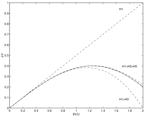
Figure 1: The spin coupling constant $J$ up to different order of transformation. H1 is the Schrieffer Wolff result, H1+H3 is the result up to the third order of the transformation, and similarly for H1+H3+H5. Solid line shows the result up to infinite order.

The contributions of $H_{1}+H_{3}$ are plotted in Fig. 1, which shows that the Kondo exchange can reverse sign. This sign oscillation is due to the ${\widetilde{V^{c}_{2}}}$ and ${\widetilde{V^{f}_{2}}}$ new terms (which are equal for the symmetric case) of Eq. (24): take for example the case where two electrons of opposite spin occupy the $f$ shell as an intermediate state. Instead of the the “down” electron, which caused the excitation, returning to the Fermi sea, the “up” electron did so, it picks up a change of sign because of the Pauli principle (the ordering of the two electrons has been interchanged). In perturbation theory, the $J_{3}$ term corresponds to a sixth order process (as mentioned earlier) of two exchanged electrons. This phenomena is the Friedel (i.e., Ruderman-Kittel) oscillations, where the polarisation periodically reverses as one proceeds to higher orders. Similar oscillations can also be observed in the renormalization group approach (Wilson 1975) in terms of energy shells. This sign oscillation is important for our analysis, as this will guarantee that the $J_{n}$ series is convergent. In this respect, it is interesting to mention that the $n$-th order canonical transformation corresponds to the $m$-th shell ($2m+1=n$) calculation in the renormalization group approach (Wilson 1975). For asymmetric cases $\varepsilon_{f}$ can be chosen in such a way to get rid of this fluctuation, for some examples see Fig. 3.

The canonical transformation can be continued up to eleventh order (Chan and Gulácsi 2001a,2004) however already in fifth order a pattern in the $J$ coefficients is observed, see Table 1 of Appendix 11, or Chan and Gulácsi (2001a,2003,2004):

$$J_{n}\>=\>(-1)^{n-1}2^{3(n-1)/2}\>\biggl{[}\frac{1}{n!}-\frac{1}{(n+1)!}\biggr{]}\>ZV^{n+1}\Big{[}(Z+A)^{2}+A^{2}\Big{]}^{(n-1)/2}\;.$$ (27)

This pattern has been proven to be valid for any order by mathematical induction. The proof is presented in detail in Appendix 11, the derivation is based on Chan and Gulácsi (2003).

Summing up the coefficients from Eq. (27) up to infinity a remarkably simple result is obtained (Chan and Gulácsi 2001a,2004):

$$J\>=\>2ZV^{2}\>\biggl{(}\frac{\sin\beta}{\beta}+\frac{\cos\beta-1}{\beta^{2}}\biggr{)}\;,$$ (28)

where

$$\beta\>=\>\sqrt{2^{3}V^{2}[(Z+A)^{2}+A^{2}]}\;.$$ (29)

For the symmetric case, where $\varepsilon_{f}=-U/2$, $J$ becomes:

$$J_{\rm sym}\>=\>V\sin(2VZ)\>+\>\frac{1}{2Z}[\cos(2VZ)-1]$$ (30)

For simplicity we consider $\epsilon(k_{F})=0$ hereafter. For this case the results for the symmetric Anderson model are plotted in Fig. 2 as a function of $U/8V$.

The two fixed points of the symmetric Anderson model can be seen clearly in Figs. 2. For $U\gg V^{2}$, Eq. (30) reduces to:

$$J_{\rm sym}\>\approx\>{\frac{U}{8}}\biggl{(}\cos{\frac{8V}{U}}-1\biggl{)}\;.$$ (31)

In the limit $U\rightarrow\infty$, this equation reduces to the well-known Schrieffer-Wolff result of the local moment or Kondo regime. However, this is not the case for smaller values of $U$.

As $U$ decreases, $V^{2}\gg U$ and $\varepsilon_{f}$ approaches $\epsilon(k_{F})$, we cross over to the mixed valence regime. Here the $s$ and $f$ bands overlap which causes the virtual excitations of the impurity energy levels (shells) and the $s-f$ multiple scattering processes to dominate. These processes cause most of the perturbative approaches to fail. However, the transformation of Chan and Gulácsi (2001a,2003,2004) is still convergent. For $U\rightarrow 0$ Eq. (30) reduces to

$$J_{\rm sym}\>\approx\>V\sin{\frac{8V}{U}}\;,$$ (32)

The strong oscillations which appear at very small values of $U$ (clearly seen in Fig. 2) are due to the multiple scattering processes.

These fluctuations are not present in the asymmetric Anderson model, as shown in Fig. 3 where Eq. (28) is plotted for different values of $\varepsilon_{f}$. When there is no $s-f$ mixing, multiple scattering processes are absent and the oscillations in $J$ disappear completely.

The 1D periodic Anderson model: In the case of the 1D periodic Anderson model, all the terms of the infinite order canonical transformation can be calculated exactly (Chan and Gulácsi 2003), details are presented in Appedix A.

The starting hamiltonian is the 1D periodic Anderson model from Eq. (14) re-written in real space:

$$H_{\mbox{\scriptsize{PAM}}}=H_{0}+H_{V}\,,$$ (33)

with

$$H_{0} = t\sum_{i,\sigma}(c^{\dagger}_{ci+1\sigma}c_{ci\sigma}+{\rm h.c.})-\mu\sum_{i,\sigma}c^{\dagger}_{ci\sigma}c_{ci\sigma}$$ (34)

$$+\varepsilon_{f}\sum_{i,\sigma}c^{\dagger}_{fi\sigma}c_{fi\sigma}+U\sum_{i}n_{fi-\sigma}n_{fi\sigma}\,,$$

$$H_{V} = V\sum_{i\sigma}(c^{\dagger}_{fi\sigma}c_{ci\sigma}+{\rm h.c})\,.$$ (35)

The transformed Hamiltonian

$$\tilde{H}{}_{\mbox{\scriptsize{PAM}}} = e^{{\cal S}}(H_{0}+H_{V})e^{-{\cal S}}$$ (36)

$$= H_{0}+\sum^{\infty}_{n=1}[1/n!-1/(n+1)!]\>H_{n}\,,$$

can be written as:

$$\tilde{H}{}_{\mbox{\scriptsize{PAM}}}=H_{0}+H_{odd}+H_{even}\,.$$ (37)

The odd hamiltonian terms are given in Eq. (48), with the exact coefficients in Eqs. (49) - (54). It can be observed that the canonical transformation generates, besides the terms which renormalize the starting Hamiltonian, three new effective interactions, $J$, $P$, and $K$, and a higher order triplet-creating term, $M$. $J$ is the Kondo coupling, and is identical to Eq. (28), the single impurity Anderson model result. $P$ a Josephson type two particle intersite tunnelling and $K$ an effective on-site Coulomb repulsion for the conduction electrons.

Eq. (61) is the final result for the even hamiltonian terms, with the exact coefficients given in Eqs. (62) - (65). It is interesting to remark that the hybridization term still exists after the transformation in the final result. However, its magnitude has been reduced from $V$ to $\approx AV^{3}/3$ (see, Eq. 62) for $V$ and $\beta$ less than one. In a real lattice, these conditions are true as the kinetic energy of the free electrons is much larger than the hybridization energy, ie $V/\mu<<1$.

We conclude this section by quoting the results of the 1D canonical transformation: The 1D periodic Anderson model, $H_{\mbox{\scriptsize{PAM}}}$ defined in Eqs. (33), (34) and (35) allows an exact mapping to an effective hamiltonian, $\tilde{H}{}_{\mbox{\scriptsize{PAM}}}$ of the form presented in Eq. (37). The transformed hamiltonian contains nine new terms, from which $J$ represents the only effective magnetic interaction. One may neglect the rest of the terms if only interested in magnetism. What remains is the exact 1D Kondo lattice hamiltonian, see Eq. (12):

$$H_{\mbox{\scriptsize{KL}}}=-t\sum_{i\sigma}(c^{\dagger}_{ci\sigma}c_{ci+1\sigma}+{\rm h.c.})+J\sum_{i}{\bf S}_{ci}{\bf\cdot}{\bf S}_{i}\,,$$ (38)

where $J$ is given by Eq. (49) or equivalent Eq. (28).

It is interesting to mention that such an infinite order canonical transformation does work for other model hamiltonians which have a similar structure to the Anderson model (so-called cylindrical quantum symmetry (Wagner 1986)). The method has been successfully applied to the 2D two band Hubbard model by Chan and Gulácsi (2000,2001b,2002). This infinite order canonical transformation method resembles the projective renormalization method introduced by Glazek and Wilson (1993).

4 An aside on notation

Several labels have arisen over the years to distinguish various aspects of the behaviour of the materials described by the Kondo lattice and periodic Anderson models. It is perhaps useful to list these various labels, and to briefly discuss their physical significance. The basic physical distinction at the heart of all the different labels may be understood in terms of the different physically relevant parameter regimes of the Kondo lattice model. From section 1, one of these regimes has strong ferromagnetic coupling: $J<0$ and $|J|/t>1$. This arises from an on-site Hund’s rule coupling between the localized electron spin and the spin of the the conduction electrons. From section 2, the second of the regimes of the Kondo lattice has weak antiferromagnetic coupling: $J>0$ and $J/t<1$. This arises from the Schrieffer-Wolff transformation of the periodic Anderson model as an effective hybridization.

A summary of the original labels used to distinguish these two regimes is presented by Varma (1976). The first regime, with strong ferromagnetic coupling, is termed the ‘mixed valence’ regime, and refers to the mixtures of ${\rm Mn}^{3+}$ and ${\rm Mn}^{4+}$ ions in the doped manganese oxide perovskites ${\rm R}_{1-x}{\rm A}_{x}{\rm MnO}_{3}$. The second regime, with weak antiferromagnetic Kondo coupling, is termed the ‘fluctuating valence’ regime, and refers to the continuous non-integral valence fluctuations at each site due to hybridization with the conduction band. Since he found these original labels somewhat mysterious, Varma (1976) proposed that a better label for the mixed valence materials would be ‘inhomogeneously mixed-valent’ to emphasize that the different ions existed as separate entities. They were then distinguished from the fluctuating valence materials, which Varma proposed to call ‘homogeneous mixed-valent’ to signify that the valence mixing occurred at each site continuously and homogeneously from site to site. These labels are now little used.

With the discovery of heavy fermion compounds, another set of labels came into use. ‘Anomalous rare earth compound’ signified the heavy fermion materials, which have hybridization between localized and extended states and are described by a weak antiferromagnetic Kondo coupling. ‘Normal rare earth compounds’ was reserved for those compounds in which the hybridization was negligible (Hewson 1993). This last labelling is now becoming less used, although it has a physical basis that further clarifies the distinction. In anomalous rare earth compounds, the level of the localized $f$ orbitals is close to the conduction electron Fermi level, and hybridization is important. The corresponding Kondo lattice has a weak antiferromagnetic coupling. In the normal rare earth compounds the $f$ level is well below that of the conduction electron Fermi level. In this case hybridization is unimportant and there is only Coulomb repulsion between localized and conduction electrons. This leads to a Kondo lattice with a ferromagnetic coupling of variable magnitude.

For ease of expression, the localized electrons will be referred to as the localized spins from now on. This describes their degrees of freedom in the Kondo lattice, and permits easy reference to all the parameter regimes of interest; it avoids the ambiguity of having ‘$f$-electrons’ occupying $d$ band orbitals when referring to Mn oxide perovskites. It also distinguishes them clearly from the conduction electrons, and the adjective ‘conduction’ may occasionally be dropped without confusion.

Chapter 1 Interactions in the Kondo Lattice Model

This chapter discusses the interactions present in the Kondo lattice in its various parameter regimes. Section 1 derives the RKKY interaction, which operates at weak-coupling. In section 2 the formation of Kondo singlets in the single impurity Kondo model is summarized, and related where possible to singlet formation in the lattice case. Section 3 discusses double-exchange ordering, which occurs in the Kondo lattice when the conduction band is under half-filled. Double-exchange has long been known to be an important mechanism in manganese oxide compounds (Zener 1951, Anderson 1955), and it is usual to consider double-exchange ordering for the Kondo lattice with a ferromagnetic coupling $J<0$. It is far less common to consider double-exchange for the antiferromagnetic $J>0$ Kondo lattice. Nevertheless, double-exchange ordering occurs also for antiferromagnetic coupling, and in section 3 a microscopic derivation is given. Since this work is new, it is discussed in some detail and forms the longest section of this chapter. Previously known results for the 1D Kondo lattice are summarized in section 4. Results for the lattice with a half-filled conduction band are given briefly in section 1. A more detailed discussion of results for the partially-filled case is given in section 2. The latter results provide an important test for the theory of the 1D Kondo lattice which is presented in chapters 4 and 5.

There are several parameter regimes of the Kondo lattice in which the dominant interaction processes may be identified. In this section these interactions are discussed. At weak-coupling $|J|/t\ll 1$, second order perturbation theory gives the Ruderman-Kittel-Kasuya-Yosida (RKKY) interaction (Ruderman and Kittel 1954, Kasuya 1956, Yosida 1957) This is an effective interaction between the localized spins which is mediated by the conduction electrons. The derivation of the RKKY interaction is given in section 1, and its divergence in 1D is discussed. Section 2 discusses Kondo singlet formation, which has a long history in the theory of systems with dilute magnetic impurities. Some of the results for dilute systems are summarized, before passing to singlet formation in the $J>0$ Kondo lattice. The RKKY interaction and Kondo singlet formation operate both in the Kondo lattice, and in systems with a very small fraction of localized spins, which model systems with dilute magnetic impurities. This is not the case for the double-exchange interaction, which operates only in the opposite case where the localized spins outnumber the conduction electrons, and occurs in the Kondo lattice with a partially-filled conduction band $n<1$. Section 3 discusses the double-exchange interaction, and determines some of its properties. Although recognized as early as 1951 as an important interaction in the perovskite manganese oxides (Zener 1951), double-exchange has only recently been discussed in relation to the $J>0$ Kondo lattice (Yanagisawa and Shimoi 1996, Honner and Gulácsi 1998b).

1 The RKKY interaction

For $J=0$, the conduction electrons in the Kondo lattice are in their non-interacting ground-state $|0\rangle$ (assumed non-degenerate), as described in section 13.A. The ground-state energy of the conduction electrons, with the Kondo lattice interaction $V_{\mbox{\scriptsize{KL}}}$ considered as a perturbation, is given by Raleigh-Schrödinger perturbation theory (Gross, Runge and Heinonen 1991) as follows:

$$E=\langle 0|V_{\mbox{\scriptsize{KL}}}|0\rangle-\sum_{n\neq 0}\frac{|\langle n|V_{\mbox{\scriptsize{KL}}}|0\rangle|^{2}}{E_{n}}+\cdots$$ (1)

where the zero of energy is chosen so that $H_{0}|0\rangle$ vanishes, and where $|n\rangle$ are non-interacting excited states with excitation energies $E_{n}>0$. The only excited states giving non-vanishing matrix elements in Eq. (1) are those of the form $|n\rangle=c^{\dagger}_{ck\sigma}c_{ck^{\prime}\sigma^{\prime}}|0\rangle$ with $|k|>k_{F}>|k^{\prime}|$. To second order, straightforward computation gives

$$E = \sum_{j,l}{\cal J}_{\mbox{\scriptsize{RKKY}}}(j-l)\,{\bf S}_{j}{\bf\cdot}{\bf S}_{l}\,,$$

$${\cal J}_{\mbox{\scriptsize{RKKY}}}(j-l) = -\frac{J^{2}}{2N^{2}}\sum_{|k^{\prime}|<k_{F}<|k|\leq\pi/a}\frac{e^{i(k^{\prime}-k)(j-l)a}}{\varepsilon(k)-\varepsilon(k^{\prime})}\,,$$ (2)

where $N$ is the number of lattice sites. Eq. (2) implies that the complete $2^{N}$-fold spin-degeneracy of the localized spins at $J=0$ is lifted by perturbation in the conduction electrons, so that the Kondo lattice is in its ground-state if the localized spins order so as to minimize $E$. Perturbation theory thus generates an effective interaction ${\cal J}_{\mbox{\scriptsize{RKKY}}}(j-l)$ between the localized spins, called the RKKY interaction, which is mediated by the conduction electrons.

The form of Eq. (2) is generic to any dimension. What differs in different dimensions is the evaluation of the summation over $k$ and $k^{\prime}$. This gives different RKKY interactions ${\cal J}_{\mbox{\scriptsize{RKKY}}}$ depending on dimensionality. The integrals may be evaluated in closed form by approximating the conduction electrons by free electrons (valid for weak-interactions for which the perturbation expansion is accurate). The calculations are carried out by Aristov (1997) with the results

$${\cal J}_{\mbox{\scriptsize{RKKY}}}(r)=\left\{\begin{array}[]{ll}\frac{m_{e}J^{2}}{2\pi}\left[{\rm Si}(2k_{F}r)-\frac{\pi}{2}\right]&{\rm 1D}\,,\\ \frac{m_{e}k_{F}^{2}J^{2}}{8\pi}\left[J_{0}(k_{F}r)Y_{0}(k_{F}r)+J_{1}(k_{F}r)Y_{1}(k_{F}r)\right]&{\rm 2D}\,,\\ \frac{m_{e}k_{F}J^{2}}{16\pi^{3}r^{3}}\left[\cos(2k_{F}r)-\frac{\sin(2k_{F}r)}{2k_{F}r}\right]&{\rm 3D}\,,\end{array}\right.$$

(4)

where $r=|(j-l)a|$ is the distance between the lattice sites $j$ and $l$, and $m_{e}$ is the bare conduction electron mass. The special functions in Eqs. (4) are the sine integral Si and the order $n$ Bessel functions of the first and second kind, $J_{n}$ and $Y_{n}$ respectively.

In 3D, the RKKY interaction decreases at large distances with $r^{-3}$, and oscillates with wave vector $2k_{F}$ (i.e. with period $\pi/k_{F}$ in real space). This favours an oscillatory alignment of the localized spins with the same periodicity. Ordering of the localized moments with wave vector $2k_{F}$ is characteristic of the RKKY interaction in any dimension, and a similar alignment is favoured in 2D. In 1D the RKKY interaction leads to a particularly strong $2k_{F}$ ordering of the localized spins. Indeed the RKKY interaction in this case is divergent: The Fourier component of ${\cal J}_{\mbox{\scriptsize{RKKY}}}$ at wave vector $k$ is defined through the Fourier transform

$${\cal J}_{\mbox{\scriptsize{RKKY}}}(j-l)=\frac{1}{2\pi}\int_{-\infty}^{\infty}dk\,{\cal J}_{\mbox{\scriptsize{RKKY}}}(k)\,e^{ik(j-l)a}\,.$$ (5)

Using the 1D form of the RKKY interaction from Eq. (4), it may be shown that (Yafet 1987)

$${\cal J}_{\mbox{\scriptsize{RKKY}}}(k)\propto\frac{1}{k}\ln\left|\frac{2k_{F}+k}{2k_{F}-k}\right|\,,$$ (6)

which has a logarithmic divergence at $2k_{F}$. ${\cal J}_{\mbox{\scriptsize{RKKY}}}(k)$ is discussed by Kittel (1968), together with the corresponding 2D and 3D forms, which do not diverge. The divergence of ${\cal J}_{\mbox{\scriptsize{RKKY}}}(k)$ in 1D is typical of the results of perturbation theory for 1D systems. The significance of the divergence is as follows: Ordering of the localized spins with wave vector $2k_{F}$ is still expected to occur in the 1D Kondo lattice at weak-coupling, much as in 3D. (This expectation is confirmed by the results of numerical simulations, cf. section 4 below). However, it is not possible to use the RKKY interaction itself to describe the $2k_{F}$ ordering in 1D, for since the interaction diverges there is no lower bound on the ground-state energy of the 1D Kondo lattice if it is described using the RKKY interaction. It is necessary to go beyond perturbation theory to describe the $2k_{F}$ correlations in the localized spins. In chapter 4 a $2k_{F}$ ordering of the localized spins is obtained at weak-coupling by using a bosonization description of the conduction electrons.

2 Kondo singlet formation

The Kondo lattice model can be considered to be the formal extension to the lattice of the single impurity Kondo hamiltonian, which has a single localized spin in a sea of conduction electrons. The single impurity Kondo hamiltonian is given by

$$H_{\rm imp}=-t\sum_{<ij>}\sum_{\sigma}c^{\dagger}_{ci\sigma}c_{cj\sigma}+J{\bf S}_{c0}{\bf\cdot}{\bf S}_{0}\,,$$ (7)

and describes a system with a magnetic impurity, modelled by a single localized spin at the origin. An antiferromagnetic Kondo coupling $J>0$ is assumed for $H_{\rm imp}$. Historically, intensive study of the single impurity Kondo model preceded that of the Kondo lattice. As a result $H_{\rm imp}$ is now well-understood, and has even been solved exactly. In the following some of the results for the single impurity Kondo hamiltonian are summarized. An emphasis is placed on results which have relevance for the Kondo lattice, and no more than a skeletal outline of the huge body of work devoted to $H_{\rm imp}$ is intended. A thorough discussion of the numerous solution methods may be found in the book by Hewson (1993), together with references.

Interest in the single impurity Kondo model arose from the observation of anomalous behaviour in the conduction electron resistivity in dilute magnetic alloys. In simple metals, and in alloys with non-magnetic impurities, the resistivity drops monotonically as the temperature $T$ decreases to $T=0$. This is because the main contribution to the resistivity at low temperatures is from electron-phonon scattering, and decreases as $T^{5}$ at low $T$. In metals with dilute magnetic impurities, such as iron in gold, the resistivity is not monotonic with temperature, but passes through a minimum before rising again as $T\rightarrow 0$. A breakthrough in understanding the occurrence of the resistance minimum was achieved by Kondo (1964), who calculated the resistivity of $H_{\rm imp}$ to third order in the coupling $J$ by standard diagrammatic perturbation theory. He found that at third order the interaction leads to singular spin scattering of the conduction electrons with the magnetic impurity, and gives a $-\log T$ contribution to the resistivity. Since $-\log T$ increases as $T\rightarrow 0$, this explained the occurrence of the resistance minimum.

Since $\log T$ diverges as $T\rightarrow 0$, it was clear that perturbation theory fails at low temperatures below the resistance minimum. Thus, while Kondo’s calculation provided a first understanding of the effect of dilute magnetic impurities, the method could not access the very low temperature regime. The problem of finding a solution valid as $T\rightarrow 0$ became known as the Kondo problem. This was essentially solved in the 1970’s by scaling arguments ; Anderson’s poor man’s scaling (Anderson 1970), and the numerical renormalization group of Wilson (1975). The basic idea is that as the temperature is lowered, the high-energy states of the conduction electrons (those far from the Fermi surface) may be eliminated. This yields an effective hamiltonian, defined for a conduction band with a reduced bandwidth, and containing a modified or ‘renormalized’ coupling between the electrons and the localized spin. The details of the scaling procedure may be found in the original papers, and are also reproduced in great detail by Hewson (1993). The results show that when the scaling reaches a characteristic Kondo temperature $T_{K}$, an initially small antiferromagnetic coupling $J>0$ becomes large, and the conduction electrons form a magnetically neutral spin-singlet with the localized spin; the magnetic impurity is quenched. The resistance minimum in dilute magnetic alloys then reflects the formation of strongly-coupled screening clouds of conduction electrons around the dilute sites which contain impurities.

The correctness of the scaling approach was confirmed in 1980 with the discovery of an exact solution to $H_{\rm imp}$ by Andrei (1980) and Wiegmann (1980), using the Bethe ansatz. The exact solution verified that the single impurity model contains one energy scale below the conduction electron bandwidth, called the Kondo temperature, which measures the energy for the quenching of the localized spin via singlet formation with the conduction electrons. The form of the Kondo temperature (see Eq. (1) of Appendix 10) is

$$T_{K}\propto\exp(-1/2\rho(\varepsilon_{F})J)\,,$$ (8)

where the density of conduction electron states at the Fermi level is

$$\rho(\varepsilon_{F})=2\sum_{k}\delta\left(\varepsilon(k)-\varepsilon(k_{F})\right)\,.$$ (9)

As a result of the existence of one energy scale, the low temperature thermodynamic properties of the model are universal functions of $T/T_{K}$. These properties are summarized in Appendix 10.

At present it is largely unclear whether, and to what extent, the results for the single impurity Kondo hamiltonian apply to the Kondo lattice. Certainly there are aspects of the single impurity solution which have no analogue in the lattice case. The most important of these is the extent of the Kondo screening cloud: When the conduction electrons screen the localized spin, forming a singlet with it, renormalization group arguments suggest that the screening cloud extends in real-space over a scale $\xi_{K}\approx v_{F}/k_{B}T_{K}$, where $v_{F}$ is the Fermi velocity of the electrons (cf. Eq. (70)) (Sørensen and Affleck 1996). Since $T_{K}$ is generally of the order of tens of degrees, the screening cloud extends over thousands of lattice spacings. This cannot occur in the lattice case, for which the extent of the screening cloud per localized spin can extend to the order of only one lattice spacing. Moreover, any screening in the lattice must be qualitatively very different from that in the single impurity problem. In the lattice the number of conduction electrons is less than, or of the order of the number of localized spins. Thus the screening of each localized spin by a large number of conduction electrons, as occurs at low temperatures in the impurity problem, cannot occur in the lattice case. Notwithstanding these problems, it is common in the Kondo lattice to propose a Kondo temperature which, analogous to the single impurity case, measures the energy scale for the formation of spin singlets around the localized spins. To understand the basis for this, it is necessary to consider the Kondo lattice at strong-coupling.

State	Energy	$S_{\mbox{\scriptsize{tot}}}$	$S^{z}_{\mbox{\scriptsize{tot}}}$	$n_{c}$
$(|\uparrow 01\rangle-|\downarrow 10\rangle)/\sqrt{2}$	$-3J/4$	0	0	1
$|\uparrow 00\rangle$	0	1/2	1/2	0
$|\downarrow 00\rangle$	0	1/2	-1/2	0
$|\uparrow 11\rangle$	0	1/2	1/2	2
$|\downarrow 11\rangle$	0	1/2	-1/2	2
$|\uparrow 10\rangle$	$J/4$	1	1	1
$(|\uparrow 01\rangle+|\downarrow 10\rangle)/\sqrt{2}$	$J/4$	1	0	1
$|\downarrow 01\rangle$	$J/4$	1	-1	1

Table 1: Eigenbasis of $V_{\mbox{\scriptsize{KL}}}$ for each lattice site $j$. The notation for the states is $|S^{z}_{j},n_{cj\uparrow},n_{cj\downarrow}\rangle$, where $S^{z}_{j}=\uparrow,\downarrow$ is the $z$ component of the localized spin at $j$, and $n_{cj\sigma}=0,1$ is the number of conduction electrons of spin $\sigma$ at $j$. ${\bf S}_{\mbox{\scriptsize{tot}}}={\bf S}_{cj}+{\bf S}_{j}$ is the total spin, and $n_{c}=n_{cj\uparrow}+n_{cj\downarrow}$ is the total number of conduction electrons. The basis consists of a singlet state, two doublets, and a triplet. The singlet state has the lowest energy for $J>0$, and the triplet states have the lowest energy for $J<0$.

At infinitely strong-coupling $|J|=\infty$, the conduction electron hopping is ineffective and the Kondo lattice hamiltonian $H_{\mbox{\scriptsize{KL}}}$ reduces to the interaction $V_{\mbox{\scriptsize{KL}}}$ of Eq. (10). It is straightforward to diagonalize $V_{\mbox{\scriptsize{KL}}}$, and the eight eigenstates per site are listed in Table 4.1. For infinite antiferromagnetic coupling $J=\infty$, the lowest energy state for each site is an on-site singlet, involving a single conduction electron pairing with a localized spin at the same site. This pairing quenches the localized spin, yielding a site with total spin zero, and this is the analogue in the lattice of the screening in the single impurity Kondo hamiltonian. The Kondo temperature is the binding energy of the singlet; the lowest excited state with the same number of conduction electrons is a triplet state, so that $k_{B}T_{K}=J$ as $J\rightarrow\infty$ (Lacroix 1985). At finite coupling the Kondo temperature is more difficult to define. In fact when the conduction band is partially-filled there is no such generally accepted definition to date. For a half-filled conduction band, there is a gap for the spin excitations, extending from infinite $J$ down to small $J$. Moreover, the ground-state of the Kondo lattice at half-filling is a total spin-singlet. (These properties are discussed further in section 1). This permits an identification of the size of the spin gap with the Kondo temperature, and at weak-coupling numerical simulations give a form identical to that for the single impurity case, but enhanced by a factor of 1.4 (Shibata, et al. 1996):

$$T_{K}\propto\exp(-1/1.4\,\rho(\varepsilon_{F})J).$$ (10)

It should be stressed that the nature of the screening in the lattice at weak-coupling is unlike that in the single impurity case.

3 Double-exchange ordering

Double-exchange was introduced in 1951 by Zener (1951) to describe ferromagnetism in the manganese oxide perovskites. Zener considered Mn oxide compounds ${\rm La}_{1-x}{\rm A}_{x}{\rm Mn}{\rm O}_{3}$, with $0<x<1$ and A $=$ Ca, Sr or Ba. The compounds contain both ${\rm Mn}^{3+}$ and ${\rm Mn}^{4+}$ ions, in concentrations $1-x$ and $x$ respectively. For $x=0$ the compounds are insulating, while at moderate doping $x\gtrsim 0.2$ they are ferromagnetic and conducting. Zener proposed that the close connection between ferromagnetism and conduction in these materials could be accounted for by supposing that the $e_{g}$ electrons on ${\rm Mn}^{3+}$ ions could hop to vacant $e_{g}$ orbitals on neighboring ${\rm Mn}^{4+}$ ions. Since hopping electrons tend to preserve their spin, and since Hund’s rule coupling strongly favours an alignment of the $e_{g}$ spin with that of the localized $t_{2g}$ electrons (cf. section 1), this hopping should favour a ferromagnetic alignment of the spins of the $t_{2g}$ electrons on neighboring Mn ions. Since the hopping of the $e_{g}$ electrons occurs through an intermediate ${\rm O}^{2-}$ ion, Zener called the ferromagnetic alignment induced by the hopping the double-exchange interaction. The name is somewhat unfortunate, since the interaction is not an exchange interaction in the usual sense, but simply reflects the tendency of hopping electrons to preserve their spin.

A microscopic derivation of the double-exchange interaction was given by Anderson and Hasegawa (1955) on a two-site Kondo lattice with a ferromagnetic coupling $J<0$, which models the Hund’s rule coupling in the Mn oxides. However, double-exchange operates regardless of the sign of the coupling, and requires only that there be more localized spins than conduction electrons; the fact that the hopping electron aligns opposite or parallel to the localized spins at each site is irrelevant to the preservation of spin while hopping. It is the latter which forces the localized spins to align. The first hints of this are in Anderson and Hasegawa’s (1955) original work; they noticed that the sign of the coupling was largely irrelevant to the ferromagnetic ordering within a semiclassical approximation for the localized spins. More recently, in the 1990s, a succession of rigorous results and numerical simulations have established a large region of ferromagnetism at partial conduction band fillings in the $J>0$ Kondo lattice (reviewed in section 2). The ferromagnetism has been attributed to double-exchange (Yanagisawa and Shimoi 1996). Not withstanding this, double-exchange is largely neglected in discussions of the $J>0$ Kondo lattice, with most papers focusing instead on the competition between RKKY interactions and Kondo singlet formation. Given this neglect, it seems worthwhile to present a detailed microscopic derivation of double-exchange for $J>0$, analogous to that for the $J<0$ Kondo lattice.

To establish double-exchange in the Kondo lattice for either sign of the coupling $J$, consider a Kondo lattice with two sites and one conduction electron. This system is equivalent to the system studied by Anderson and Hasegawa (1955), in which double-exchange ordering was shown to occur within a semiclassical approximation for the localized spins. Apart from minor differences in some numerical factors, double-exchange was found to operate independent of the sign of the coupling $J$ in the semiclassical case. Double-exchange ordering was also demonstrated by Anderson and Hasegawa for quantum localized spins, but in a reduced (4-dimensional) Hilbert space. The reduced space is sufficient if the coupling $J<0$ is ferromagnetic, and this was the case of interest to Anderson and Hasegawa who considered the Mn oxides. For antiferromagnetic Kondo coupling $J>0$, it is no longer sufficient to operate in a 4-dimensional Hilbert space. In the following the complete 16-dimensional Hilbert space of the system is considered.

States of the two site Kondo lattice may be written

$$|S^{z}_{1},n_{c1\uparrow},n_{c1\downarrow}:S^{z}_{2},n_{c2\uparrow},n_{c2\downarrow}\rangle\;,$$

in a straightforward generalization of the single-site states used in Table 4.1; $S^{z}_{j}=\uparrow,\downarrow$ is the $z$ component of the localized spin at site $j=1,2$, and $n_{cj\sigma}=0,1$ is the number of conduction electrons of spin $\sigma$ at site $j$. A single conduction electron can be in one of the 4 states $n_{cj\sigma}$, and for each of these configurations there are 4 possible configurations for the localized spins $S^{z}_{1}S^{z}_{2}$: $\uparrow\uparrow$, $\uparrow\downarrow$, $\downarrow\uparrow$, $\downarrow\downarrow$. Thus a basis for the two site Kondo lattice with one conduction electron has 16 elements. The $16\times 16$ matrix of the Kondo lattice hamiltonian Eq. (12) operating on basis elements $|S^{z}_{1},n_{c1\uparrow},n_{c1\downarrow}:S^{z}_{2},n_{c2\uparrow},n_{c2\downarrow}\rangle$ is easily constructed, and the eigenvalues and eigenvectors are obtained in analytic form. This gives a complete solution of the system, and may be used to analyse the ground-state properties as a function of $t/J$.

For ferromagnetic coupling $J<0$ the ground-state properties are relatively simple, and are well-described within a semiclassical approximation (Anderson and Hasegawa 1955). This case is included in the discussion here because the analysis for $J<0$ aids in identifying similar behaviour in the more complicated case of antiferromagnetic coupling. The ground-state energy of the system for infinite coupling $J\rightarrow-\infty$ is $-|J|/4$. This corresponds to a triplet pairing between the conduction electron and a localized spin at the same site, together with an unpaired localized spin at the other site. There are 12 distinct configurations of states of this form, and the ground-state is 12-fold degenerate at $J=-\infty$. Conduction electron hopping partially lifts this degeneracy. For example, the state $|\uparrow 10:\uparrow 00\rangle$ is preferred over the state $|\uparrow 10:\downarrow 00\rangle$ because the conduction electron can hop to site 2 while maintaining its spin parallel to the localized spin at the new site. The ground-state energy for finite ferromagnetic coupling is

$$E_{0}=-\frac{|J|}{4}-t\,,\quad\quad J<0\,,$$ (11)

and the ground-state is only 4-fold degenerate. This degeneracy may be understood by considering the total spin operator ${\bf S}_{\mbox{\scriptsize{tot}}}=\sum_{j}{\bf S}_{j}+{\bf S}_{cj}$. Each of the four ground-states is an eigenvector of $S_{\mbox{\scriptsize{tot}}}^{2}$ with total spin $3/2$, and the ground-state degeneracy simply reflects the 4 choices of the $z$ component $S^{z}_{\mbox{\scriptsize{tot}}}$ of the total spin. The Kondo lattice hamiltonian Eq. (12) does not mix states with different values of $S^{z}_{\mbox{\scriptsize{tot}}}$, and it suffices to consider a subspace in which $S^{z}_{\mbox{\scriptsize{tot}}}$ is fixed. In the subspace with $S^{z}_{\mbox{\scriptsize{tot}}}=3/2$, the ground-state is unique and takes a particularly simple form:

$$|\psi_{0}\rangle=\frac{1}{\sqrt{2}}\left(|\uparrow 10:\,\uparrow 00\rangle+|\uparrow 00:\,\uparrow 10\rangle\right)\quad\,\,J<0\,.$$ (12)

This state is the prototype for double-exchange ordering. For finite ferromagnetic coupling the system minimizes energy by conduction electron hopping, and by having the conduction electron spin aligned parallel to the localized spin at each site. Since hopping electrons tend to conserve their spin, called coherent electron hopping, the minimal energy is obtained if all the localized spins align with the conduction electron spin. The ferromagnetic ordering induced on the localized spins by coherent conduction electron hopping is the double-exchange interaction.

Consider now an antiferromagnetic Kondo coupling $J>0$. In this case the conduction electron spin tends to align opposite to the localized spin. At infinite coupling $J=\infty$, the ground-state energy is $-3J/4$ and the ground-state consists of a singlet pairing between the conduction electron and a localized spin at the same site (i.e. a localized Kondo singlet), together with an unpaired localized spin at the other site. The ground-state is 4-fold degenerate. Conduction electron hopping partially lifts this degeneracy, similar to the case for ferromagnetic coupling. For finite antiferromagnetic coupling the ground-state energy is given by the solution of the $16\times 16$ matrix as

$$E_{0}=-\frac{J}{4}-\frac{1}{2}\sqrt{J^{2}+2Jt+4t^{2}}\,,\quad\quad J>0\,,$$ (13)

and the ground-state is two-fold degenerate. Both of the ground-states are eigenstates of $S^{2}_{\mbox{\scriptsize{tot}}}$ with total spin 1/2. The degeneracy is due to the two choices of $S^{z}_{\mbox{\scriptsize{tot}}}$, and as for $J<0$ it suffices to consider a subspace with fixed $S^{z}_{\mbox{\scriptsize{tot}}}$. The unique ground-state with $S^{z}_{\mbox{\scriptsize{tot}}}=1/2$ is given by

$$|\psi_{0}\rangle \propto |\,s_{1}\uparrow\rangle+|\uparrow s_{2}\rangle$$ (14)

$$+ \frac{t}{J/4-E_{0}}\left\{|\uparrow 01:\,\uparrow 00\rangle+|\uparrow 00:\,\uparrow 01\rangle\right.$$

$$\left.\quad-|\uparrow 10:\,\downarrow 00\rangle-|\downarrow 00:\,\uparrow 10\rangle\right\}\,\quad\,\,J>0\,.$$

The proportionality constant is the normalization, and the $J=\infty$ behaviour has been separated out using the localized Kondo singlet states:

$$|\,s_{1}\uparrow\rangle = |\uparrow 01:\,\uparrow 00\rangle-|\downarrow 10:\,\uparrow 00\rangle\,,$$

$$|\uparrow s_{2}\rangle = |\uparrow 00:\,\uparrow 01\rangle-|\uparrow 00:\,\downarrow 10\rangle\,.$$ (15)

The ground-state Eq. (14) involves six basis elements, and falls outside the 4-dimensional space used by Anderson and Hasegawa (1955) to establish double-exchange for ferromagnetic coupling $J<0$. Although somewhat obscured, double-exchange ferromagnetic ordering of the localized spins is present also in the ground-state of the $J>0$ Kondo lattice, as can be shown in two steps. First, the correlation between the localized spins in the ground-state Eq. (14) is calculated. Second the $J>0$ ground-state is rewritten in a form in which double-exchange is made manifest, i.e. similar in form to Eq. (12), but with the conduction electron spin aligning opposite to the localized spins.

The ground-state correlation between the localized spins is given by

$$\frac{\langle\psi_{0}|S^{\alpha}_{1}S^{\alpha}_{2}|\psi_{0}\rangle}{\langle\psi_{0}|\psi_{0}\rangle}=\frac{1}{4}\left[1+\frac{t}{J/4-E_{0}}+\frac{J/4-E_{0}}{t}\right]^{-1}$$ (16)

where $\alpha=x,y,$ or $z$. The correlation is ferromagnetic for each component of the spin, and the contribution from each component is identical. The full spin-spin correlation between the localized spins is plotted in Fig. 4 as a function of $t/J$. The ferromagnetic correlation between the localized spins grows quickly from zero at infinite coupling, and when $t=J$ is already at 90% of the possible maximum of 1/4. For comparison, Fig. 4 also includes the correlation between the localized spins in the ground-state for $J<0$. The result for $J<0$ coincides with the correlation for any sign of the coupling within a semiclassical approximation for the localized spins (Anderson and Hasegawa 1955).

It remains to show that the ferromagnetic ordering between the localized spins for $J>0$ is due to the double-exchange interaction. Double-exchange in the $z$ direction of the spin is manifest in Eq. (14) in the third and fourth states:

$$|{\rm de}_{z}\rangle=|\uparrow 01:\,\uparrow 00\rangle+|\uparrow 00:\,\uparrow 01\rangle\,.$$ (17)

This has the form of Eq. (12), and differs only in that for antiferromagnetic coupling $J>0$, the conduction electron spin aligns opposite to the localized spins. The remaining terms in the $J>0$ ground-state, Eq. (14), represent double-exchange ordering along the $x$ and $y$ spin axes, together with residual localized Kondo singlets. To see this, introduce the eigenstates of $S^{x}=(S^{+}+S^{-})/2$ and $S^{y}=(S^{+}-S^{-})/2i$. These are defined in terms of the spin $z$ basis by:

$$|\uparrow_{x}\rangle = (|\downarrow\rangle+|\uparrow\rangle)/\sqrt{2}\,,\quad|\uparrow_{y}\rangle=i(i|\downarrow\rangle+|\uparrow\rangle)/\sqrt{2}\,,$$

$$|\downarrow_{x}\rangle = (|\downarrow\rangle-|\uparrow\rangle)/\sqrt{2}\,,\quad|\downarrow_{y}\rangle=i(i|\downarrow\rangle-|\uparrow\rangle)/\sqrt{2}\,.$$

(The convention for the notation is that spins without a subscript always refer to the $z$ direction.) The arbitrary phases in these states have been chosen because they are convenient for working in the $S^{z}_{\mbox{\scriptsize{tot}}}=1/2$ subspace. Double-exchange in the $\alpha=x,y$ spin directions, and with an antiferromagnetic coupling $J>0$, is described by

$$|{\rm de}_{\alpha}\rangle = ([\,|\uparrow_{\alpha}01:\,\uparrow_{\alpha}00\rangle+|\uparrow_{\alpha}00:\,\uparrow_{\alpha}01\rangle]$$ (18)

$$+ [\,|\downarrow_{\alpha}10:\,\downarrow_{\alpha}00\rangle+|\downarrow_{\alpha}00:\,\downarrow_{\alpha}10\rangle])/\sqrt{2}\,.$$

In these states the conduction electron occupation numbers refer to the spin direction $\alpha$: $n_{cj\sigma_{\alpha}}=0,1$ gives the number of conduction electrons with spin $\uparrow_{\alpha}$ or $\downarrow_{\alpha}$ at site $j$. The states $|{\rm de}_{\alpha}\rangle$ for $\alpha=x,y$ have the same form, and the same normalization, as that of Eq. (17) for double-exchange in the $z$ direction. The only difference is that the $S^{\alpha}_{\mbox{\scriptsize{tot}}}=1/2$ and $-1/2$ double-exchange forms (enclosed by the square brackets in Eq. (18)) have been summed, which is the appropriate combination for the $S^{z}_{\mbox{\scriptsize{tot}}}=1/2$ subpace. The ground-state Eq. (14) for $J>0$ may now be written as

$$|\psi_{0}\rangle \propto \left(1-\frac{t}{J/4-E_{0}}\right)(|\,s_{1}\uparrow\rangle+|\uparrow s_{2}\rangle)$$ (19)

$$+ \frac{t}{J/4-E_{0}}(|{\rm de}_{x}\rangle+|{\rm de}_{y}\rangle+|{\rm de}_{z}\rangle)\,.$$

The proportionality constant is the normalization, and coincides with that in Eq. (14). As $t/J$ increases, $|\psi_{0}\rangle$ describes weight being taken away from the localized Kondo singlet states $|\,s_{1}\uparrow\rangle$ and $|\uparrow s_{2}\rangle$, which define the non-magnetic $J=\infty$ ground-state. The weight is shifted in equal proportion to the double-exchange terms $|{\rm de}_{\alpha}\rangle$ along the three spin axes $\alpha=x,y,z$. This produces the spin-isotropic ferromagnetic ordering between the localized spins, as in Fig. 4. Eq. (19) makes it clear that the ferromagnetic ordering observed in Fig. 4 for $J>0$ is due to the double-exchange interaction, as for the $J<0$ case.

It is useful to comment on the differences between the ground-states for different signs of the coupling $J$. For ferromagnetic coupling the double-exchange ordering can be described using just the spin $z$ direction, at least in the subspace with maximal $S^{z}_{\mbox{\scriptsize{tot}}}$. For antiferromagnetic coupling all spin directions were required. This difference is superficial, and while it increases the complexity of the description for $J>0$, there is no difference in the physics. The reason the simple form Eq. (12) can be obtained for $J<0$ is because the ground-state has maximal $S^{2}_{\mbox{\scriptsize{tot}}}$ corresponding to fully saturated ferromagnetism. Thus, by describing the system in the subspace with maximal $S^{z}_{\mbox{\scriptsize{tot}}}$, all the spins in the system are aligned, and the spin-flip part $J(S^{-}_{cj}S^{+}_{j}+S^{+}_{cj}S^{-}_{j})/2$ of the hamiltonian Eq. (12) becomes ineffective. For antiferromagnetic coupling $J<0$ the ferromagnetism is not saturated. The localized spins align, but the conduction electron spin is opposite to that of the localized spins. In this case it is not possible to choose a subspace of $S^{z}_{\mbox{\scriptsize{tot}}}$ in which the spin-flip part of the hamiltonian becomes ineffective: All spin directions are required to extract the double-exchange ordering in the ground-state for $J>0$. Nonetheless the physics of the ordering remains unaffected. For example, similar complications ensue for $J<0$ if one chooses the subspace with $S^{z}_{\mbox{\scriptsize{tot}}}=1/2$.

An intrinsic difference between the ground-states for different signs of the coupling is the residual weight attached to the localized Kondo singlets when $J>0$. This is due to the increased gain in energy $-3J/4$ for a Kondo singlet, over the energy gain $-|J|/4$ for a triplet state when $J<0$. The energy gain per site due to double exchange is $-|J|/4$ for either sign of the coupling. Thus, when $J<0$ the system gains just as much energy by triplet formation as by double-exchange, and there is no competition between the two. This is clear in the ground-state Eq. (12), which is consistent both with double-exchange ordering, and with a superposition of triplet formation at each site. As a result of this, the ground-states for $J<0$ do not evolve as $t/J$ increases, and the maximum ferromagnetic ordering between the localized spins sets in with $t/J$ arbitrarily small, as is clear from Fig. 4. For $J>0$ there is a competition between singlet formation and double-exchange ordering. When $t/J$ is small Kondo singlet formation dominates, and the ferromagnetic correlation between the localized spins vanishes as $t/J\rightarrow 0$. As $t/J$ increases, there is a larger energy gain for conduction electron hopping and this favours double-exchange. At large $t/J$ double-exchange dominates, and no residual Kondo singlets remain. The localized spins are then strongly ferromagnetically ordered. The crossover between the limiting behaviours is shown in Fig. 4, and is characterized by $t/(J/4-E_{0})$ with $E_{0}$ given by Eq. (13).

4 1D Kondo lattice results

The Kondo lattice model has been studied intensively for over two decades. Notwithstanding this effort, reliable results on the Kondo lattice are few. The extension to the lattice case of methods developed for the single impurity Kondo model are either impossible, as in the Bethe ansatz solution of Andrei (1980) and Wiegmann (1980), or involve uncontrolled approximations. Primary examples of the latter are $1/N$ expansions, the slave boson method, and Gutzwiller approximations. (See Tsunetsugu, Sigrist and Ueda (1997) for references and discussion.) These methods have been quite successful in describing the formation of a coherent band of heavy quasiparticles, as is observed in the heavy fermion compounds. However, the methods taken over from the single impurity Kondo model focus on local correlations only, and have offered no consensus on the ground-state phases of the Kondo lattice. Thus, while the various methods developed on the basis of the single impurity model appear to capture some of the physics of the lattice problem, it is a priori unclear as to which aspects of the various solutions are reliable, and which are not.

For the 1D Kondo lattice, some rigorous results have appeared in the 1990s, and have been supplemented by the results of a variety of numerical simulations. All these results are in substantial agreement, and give support to the view that the broad features of the ground-state phase diagram of the 1D Kondo lattice are now known. It is useful for later reference to summarize these results, and to provide a picture of the properties of the 1D Kondo lattice as it was understood in the early 1990s.

The main focus of this review is the conventional 1D Kondo lattice model as defined in Eq. (12). Variants of the conventional spin-isotropic model, such as the inclusion of nearest-neighbour (White and Affleck 1996, Sikkema, Affleck and White 1997, Coleman, Georges and Tsvelick 1997) or considering spin-anisotropic interaction (Shibata, Ishii and Ueda 1995, Zachar, Kivelson and Emery 1996, Novais, it et al. 2002a,2002b), do not constitute the main topic of discussion of this review Even though some of these extensions of the conventional Kondo lattice will be discussed at later stages of this review.

Hence, section 1 only contains a brief discussion of results for the 1D Kondo lattice with a half-filled conduction band. Since the lattice with a partially-filled (ie less than half-filled) conduction band is the focus of interest in chapters 4 and 5, section 2 contains a detailed discussion of previously known results for the 1D Kondo lattice at partial conduction band filling.

1 Half-filled conduction band

The Kondo lattice with a half-filled conduction band is thought by some (Yu and White 1993, Wang, Li and Lee 1993, Guerrero and Yu 1995) to be an effective model for the class of Kondo insulators. As discussed in section 2, the Kondo insulators are small gap semiconductors, in which the gap derives from a hybridization between singly-occupied localized $f$-orbitals, and a half-filled conduction band (Aeppli and Fisk 1992, Fisk, et al. 1995). There are some doubts as to whether the Kondo insulators are in the local moment regime (Varma 1994), and therefore some question as to whether the Kondo lattice is applicable, or whether the more fundamental periodic Anderson model is required (cf. section 2). This issue will not be addressed here.

Half-filling is defined by $n=N_{e}/N=1$, where $N_{e}$ is the number of conduction electrons and $N$ the number of lattice sites (i.e. the number of localized spins). A rigorous theorem holds for the half-filled Kondo lattice in any dimension on a bipartite lattice (Tsunetsugu, et al. 1992, Shen 1996, Tsunetsugu, Sigrist and Ueda 1997): For antiferromagnetic coupling $J>0$ the ground-state is unique and has zero total spin $S_{\mbox{\scriptsize{tot}}}=0$ (i.e. the ground-state is a total spin singlet). The same conclusion holds for ferromagnetic coupling $J<0$ provided the two sublattices have the same number of sites. Beyond the rigorous proof that the ground-state is a total spin singlet in any dimension, there is substantial evidence that the ground-state also has a spin gap at least in 1D. The ground-state of the half-filled 1D Kondo lattice thus forms a spin-liquid. To discuss the evidence for this, it is convenient to consider the $J>0$ and $J<0$ cases separately.

Antiferromagnetic coupling $J>0$: At infinite coupling $J=\infty$ the ground-state at half-filling consists of $N$ on-site Kondo singlets (cf. Table 4.1). There is a spin gap of size $J$ to an on-site triplet state, and a larger charge gap of $3J/2$, corresponding to the hopping of a conduction electron to a neighboring site. The persistence of the spin gap (and a larger charge gap) down to arbitrarily small coupling strengths $J>0$ has been established by the following numerical simulations: quantum Monte Carlo at $J/t=1.6$ (Fye and Scalapino 1990); exact diagonalization on systems of up to 10 sites, and over the full range of couplings $J>0$ (Tsunetsugu, et al. 1992); density-matrix renormalization group studies on lattices of up to 24 sites and over a wide range of coupling strengths (Yu and White 1993). The numerical results are further supported by approximate analytic techniques; Gutzwiller-projected mean-field solutions (Wang, Li and Lee 1993), and a mapping of the Kondo lattice to a nonlinear sigma model at weak-coupling, within a semiclassical approximation for the localized spins (Tsvelik 1994). As noted in section 2, the singlet ground-state and spin gap in the half-filled Kondo lattice permits a formal identification of the Kondo temperature as the energy of the spin gap. At strong-coupling this is linear in $J$ and at weak-coupling takes an exponential form Eq. (10) which is similar to, but enhanced over, the single impurity result Eq. (8).

Ferromagnetic coupling $J<0$: Substantially less work has been done on the half-filled Kondo lattice with $J<0$. Exact-diagonalization results in 1D, together with finite size scaling (Tsunetsugu, et al. 1992, Shibata, et al. 1996), show that there exists a spin gap for $J<0$ as for the half-filled $J>0$ Kondo lattice. Nevertheless the nature of the gap for $J<0$ is different. For $J>0$, the strong-coupling behaviour is that of the Kondo spin liquid, while for $J<0$ it scales to a spin 1 chain, and reduces to a Haldane gap state at strong-coupling; instead of the spin gap increasing as $J\rightarrow-\infty$, it decreases at large $J$ (Tsunetsugu, et al. 1992).

Correlations: The correlations between nearest-neighbour localized spins in the half-filled 1D KLM are antiferromagnetic for any sign of the coupling. This may be understood beginning from the $|J|=\infty$ limits where there is one conduction electron localized at each site. At strong but finite coupling there is weak virtual conduction electron hopping to neighboring sites. By the Pauli principle, this is possible only if the conduction electron on the neighboring site has opposite spin. For strong but finite ferromagnetic or antiferromagnetic coupling, the weak antiferromagnetism of the localized conduction electrons induces a similar antiferromagnetic ordering on the underlying localized spins. Strong antiferromagnetism at weak-coupling is expected on the basis of the RKKY interaction which oscillates in sign with wave vector $2k_{F}$ (cf. section 1). At half-filling $k_{F}=\pi/2a$, and so the RKKY interaction changes sign at neighboring lattice sites. These expectations are supported by the results of numerical simulations for $J>0$ (Fye and Scalapino 1990, Yu and White 1993), and by perturbation theory at large ferromagnetic couplings (Tsunetsugu, et al. 1992).

Higher dimensions: As mentioned earlier, a great deal of work has been carried out on the one dimensional Kondo lattice model for over two decades. However, in higher dimensions results are few, and most of them are numerical studies for the half filled band, spin liquid phase. These studies show that the spin liquid phase, at large $J$, becomes unstable against antiferromagnetic long-range order formation at small $J$, at a finite $J_{c}$. Above the transition, a popular scenario (Pépin and Lavagna 1999, Lavagna and Pépin 2000) involves antiferromagnetic spin fluctuations coupling to the Fermi liquid properties. The low temperature physics of this is controlled by a collective mode that softens at the antiferromagnetic transition (Lavagna and Pépin 2000). The transition occurs at $J_{c}\approx 1.4$ for the two dimensional case and around $J_{c}\approx 1.8-2.0$ for the three dimensional one. The estimates for the critical coupling in two dimensions have been confirmed by several different calculations, such as mean-field approaches (Lacroix and Cyrot 1979, Zhang and Yu 2000, Jurecka and Brening 2001), quantum Monte Carlo simulations (Wang, Li and Lee 1994, Assad 1999, Capponi and Assad 2001) and series expansions (Shi et al. 1995, Zheng and Oitmaa 2003). In the three dimensional case only series expansions have been implemented until now (Shi et al. 1995, Zheng and Oitmaa 2003). It is interesting to remark that the series expansion methods, both in two and three dimensions, suggest that the spin excitations becomes gapless at the quantum critical point, while the charge excitations ramain gapped. This may suggest that similarly to the one dimensional case, the nonlinear sigma model is the appropriate low energy theory also in hiher dimensions.

2 Partially-filled conduction band

Results for the 1D Kondo lattice with a partially-filled conduction band $n=N_{e}/N<1$ fall into two categories; rigorous results proved using the Perron-Frobenius theorem, and results obtained by numerical simulations. These results are summarized in turn. Most apply to the case of antiferromagnetic coupling $J>0$.

Rigorous results in limiting cases: Two rigorous results have been proven for the 1D Kondo lattice hamiltonian, Eq. (12).

(i) The Kondo lattice with one conduction electron. Sigrist, Tsunetsugu and Ueda (1991) proved that the ground-state of the Kondo lattice with one conduction electron forms an incompletely saturated ferromagnet, with total spin $S_{\mbox{\scriptsize{tot}}}=(N-1)/2$, for $J>0$, and forms a fully saturated ferromagnet, $S_{\mbox{\scriptsize{tot}}}=(N+1)/2$, for $J<0$. For $J<0$, the theorem is trivial, since the spin-flip part of the Kondo lattice interaction is ineffective, much as for the two-site lattice discussed in section 3; the ground-state consists of an alignment of all the localized spins, together with the conduction electron in a zero momentum Bloch state and with spin opposite to that of the localized spins. For antiferromagnetic coupling $J>0$ the theorem is non-trivial, and is proved by adopting a special phase convention for the conduction electron states, and then applying the Perron-Frobenius theorem of matrix theory (Sigrist, Tsunetsugu and Ueda 1991). The Perron-Frobenius theorem also proves that the ground-state is unique, except for the usual $2S_{\mbox{\scriptsize{tot}}}+1$ choices for the $z$ component $S^{z}_{\mbox{\scriptsize{tot}}}$ of the total spin. A detailed presentation of the proof, together with the required matrix theory, is given by Yanagisawa and Harigaya (1994). The theorem holds in any dimension, and for all finite coupling strengths $0<J<\infty$. It applies also if the conduction electron hopping goes beyond nearest-neighbour, provided that the hopping amplitudes remain negative.

Sigrist et al. (1991) also constructed the maximal $S_{\mbox{\scriptsize{tot}}}^{z}$ ground-state of the $J>0$ Kondo lattice with one conduction electron, and used it to investigate some of the ground-state properties. The conduction electron in the lattice of localized spins is a spin polaron. It moves dressed by a polarization cloud of localized spins, which tend to align antiparallel to the conduction electron spin. The effective mass $m^{*}$ of the electron is thereby slightly enhanced, and varies from $m^{*}=m_{e}$ at $J=0$ to $m^{*}=2m_{e}$ as $J\rightarrow\infty$, where $m_{e}$ is the bare electron mass. The spatial extension of the polarization cloud is given by the correlation between the conduction electron spin and nearby localized spins. As $J\rightarrow\infty$ the extension shrinks down to on-site correlation only, as the conduction electron localizes in an on-site Kondo singlet. For small $J$, the correlation decays exponentially with a coherence length $\sqrt{2t/J}$, which characterizes the extension of the polarization cloud.

Using exact diagonalization on systems of up to 14 sites, Sigrist, Ueda, and Tsunetsugu (1992a) later investigated the interactions between spin polarons in the $J>0$ 1D Kondo lattice with two conduction electrons. As $J$ is increased, the electrons separate, forming separate spin polarization clouds, and form strongly repulsive on-site Kondo singlets as $J\rightarrow\infty$

(ii) Strong-coupling expansion. For partial conduction band filling $n<1$, the $J=\infty$ ground-state consists of $N_{e}$ on-site Kondo singlets, and $N-N_{e}$ free unpaired localized spins (cf. Table 4.1). The ground-state has a $2^{N-N_{e}}$–fold spin degeneracy. Introducing corrections of order $t/J$, the on-site Kondo singlets hop to nearest-neighbour unpaired sites with amplitude $-t/2$ (Hirsch 1984). Hopping Kondo singlets alter the charge configuration, but not the spin configuration: The unpaired localized spin and the Kondo singlet simply exchange sites, with no flipping of the localized spin. Thus at ${\cal O}(t/J)$ the charge and spin degrees of freedom are decoupled, and the picture formed by focusing on mobile Kondo singlets up to ${\cal O}(t/J)^{2}$ is given by Hirsch (1984).

A qualitatively different picture emerges by considering ${\cal O}(t/J)^{2}$ corrections which alter the spin configuration. Sigrist, Tsunetsugu, Ueda and Rice (1992b) performed a systematic expansion in powers of $t/J$ out of the $J=\infty$ ground-state. They neglected the higher-energy excitations to on-site triplets, which cost an energy $J$, and neglected the states with two conduction electrons at the same site, which cost an energy $3J/2$ corresponding to the destruction of two Kondo singlets. At order $(t/J)^{2}$, Sigrist et al. obtain a series of complicated hopping processes, one of which alters the spin configuration. Using the Perron-Frobenius theorem, it is then proved that the ground-state spin degeneracy is lifted at order $(t/J)^{2}$ to give an incompletely saturated ferromagnet with total spin $(N-N_{e})/2$ corresponding to the alignment of all unpaired localized spins (Sigrist, et al. 1992b). The theorem holds for all partial conduction band fillings $n<1$.

The strong-coupling result was later extended by Yanagisawa and Harigaya (1994), who used the Perron-Frobenius theorem to prove a similar result for the partially-filled 1D Kondo lattice with a strong conduction electron Hubbard repulsion $U\sum_{j}n_{cj\uparrow}n_{cj\downarrow}$ (cf. Eq. (12)) added to the standard hamiltonian Eq. (12): As $U\rightarrow\infty$, the ground-state of the Kondo lattice for $n<1$ has total spin $S_{\mbox{\scriptsize{tot}}}=(N-N_{e})/2$ for all antiferromagnetic couplings $J>0$, and $S_{\mbox{\scriptsize{tot}}}=(N+N_{e})/2$ for all ferromagnetic couplings $J<0$. Thus ferromagnetism occupies the whole of the phase diagram ($0<n<1$, $J\neq 0$) if there is a strong Hubbard repulsion between the conduction electrons.

Results by numerical simulations: The rigorous results for the Kondo lattice apply only in limiting parameter regimes; vanishing conduction band filling $n\rightarrow 0$, and the strong-coupling limit $t/J\rightarrow 0$. In both these limits a ferromagnetic ordering is favoured; incompletely saturated ferromagnetism for $J>0$, and fully saturated ferromagnetism for $J<0$. The remainder of the ground-state phase diagram was tackled using numerical simulations.

Antiferromagnetic coupling: Several numerical studies by a variety of different methods have been carried out on the partially-filled 1D Kondo lattice in the early 1990s. For antiferromagnetic couplings $J>0$, the earlier studies have been completed by: (i) Troyer and Würtz (1993), who used quantum Monte Carlo on systems of up to 24 sites, and at conduction band fillings $n=1/3$ and $2/3$. (ii) Tsunetsugu, Sigrist and Ueda (1993), who used exact diagonalization on systems of up to 9 sites and over the full range of fillings $0<n<1$. (iii) Moukouri and Caron (1995), who used the density-matrix renormalization group on systems of up to 75 sites at $n=0.7$. (iv) Caprara and Rosengren (1997), who used the infinite-size version of the density-matrix renormalization group on systems of up to 202 sites, and over a range of small fillings $0<n\leq 1/2$.

The results of all these studies are in very good agreement with each other, as well as with the rigorous results, and the basic picture they present is now generally accepted. From the numerical results on larger systems ((i), (iii), (iv)), the 1D Kondo lattice with $n<1$ and $J>0$ shows a ferromagnetic ordering of the localized spins at stronger couplings. This is identified by the structure factor of the localized spins (i.e. the Fourier transform of the real space correlation function for the localized spins) (Troyer and Würtz 1993):

$$C(k)=\frac{1}{N}\sum_{j,l}^{N}e^{ik(j-l)a}\,\langle S^{z}_{j}S^{z}_{l}\rangle\,.$$ (20)

The simulations on the larger systems show a peak in $C(k)$ at $k=0$, which indicates an alignment of the localized spins. This is accompanied by a very weak ferromagnetic correlation in the spin structure factor for the conduction electrons. As the coupling is lowered, the Kondo lattice undergoes a transition to a paramagnetic phase at a critical coupling $J_{c}$ in the weak to intermediate range ($0<J_{c}/t\lesssim 4$). The paramagnetic phase is characterized by a peak in the localized spin structure factor at $2k_{F}$, where $k_{F}$ is the conduction electron Fermi momentum. The correlations between the localized spins in the paramagnetic phase are characteristic of the RKKY interaction, though recall that the RKKY interaction diverges in 1D, as is typical of perturbative expansions in low dimensions (cf. section 1 and the discussion given there). In the paramagnetic phase the correlations in the conduction electron spins again weakly track those of the localized spins, so there is a very weak $2k_{F}$ peak in the structure factor of the conduction electron spins. The critical coupling $J_{c}$ marking the ferromagnetic-paramagnetic transition depends on the filling, $J_{c}=J_{c}(n)$, and is identified in the numerical studies (i), (iii) and (iv) as the point where the intensity of the $k=0$ peak in $C(k)$ is equal to the intensity of the $k=2k_{F}$ peak; at stronger couplings the $k=0$ peak dominates (ferromagnetism), and at weaker couplings the RKKY-like $k=2k_{F}$ peak dominates (paramagnetism). The obtained transition points are shown in Fig. 5.

The exact diagonalization study (ii) of Tsunetsugu et al. (1993) presents the same phase diagram as that obtained by the studies on larger systems; some representative phase transition points obtained by exact digonalization are shown in Fig. 5. Contrary to the other studies, the transition points in this case are obtained by calculating the total spin of the system. The transition points mark the values at which the total spin changes from incompletely saturated ferromagnetism $S_{\mbox{\scriptsize{tot}}}=(N-N_{e})/2$ to the paramagnetic value of minimal total spin $S_{\mbox{\scriptsize{tot}}}=0$ or $1/2$ depending on whether $N-N_{e}$ is even or odd. At smaller fillings, there is a small crossover regime between these extremities which signifies a continuous phase transition. The analytic work of chapter 4 predicts this type of ferromagnetic-paramagnetic transition for the 1D Kondo lattice. At larger fillings the crossover is sharp, and signifies a first-order transition. The results of chapter 4 dispute this as a property in a thermodynamically large Kondo lattice, and the sharp crossover must be due to the small system sizes $N\leq 9$ for which the exact diagonalization method is practicable. Indeed, in their review Tsunetsugu, Sigrist and Ueda (1997), the authors of the exact diagonalization study state that the small size of the systems makes it difficult to judge the type of transition on the basis of their results.

The recent numerical results (McCulloch, et al. 1999, 2001, 2002) confirmed the above results. The high accuracy of the modern numerical algorithms allowed the whole phase diagram to be mapped out for all values of electron doping levels, see section 5.

Ferromagnetic coupling. For ferromagnetic couplings $J<0$, the Kondo lattice has been studied by Dagotto’s group (Dagotto, et al. 1998, Yunoki, et al. 1998) using a variety of numerical methods, including quantum Monte Carlo, the density-matrix renormalization group, and Lanczos methods. The general phase diagram they obtain, from studies of the Kondo lattice in one-, two- and infinite-dimensions, and for both quantum and semiclassical localized spins, is as follows: At stronger coupling the ground-state is ferromagnetic, as identified by a $k=0$ peak in the structure factor $C(k)$ of the localized spins (cf. Eq. (20)). At weaker coupling the ground-state is a paramagnet, with incommensurate correlations in $C(k)$ which usually correspond to $2k_{F}$, as expected on the basis of the RKKY interaction. The crossover between the ferromagnetic and paramagnetic phases occurs at a critical coupling dependent on filling. This transition line has the same general shape as that for $J>0$ at small fillings (cf. Fig. 5), but turns upward as $n\rightarrow 1$ and approaches the half-filling line asymptotically (cf. Fig. 13 for some representative points). Dagotto’s group also find a phase separated region close to half-filling at strong coupling.

The status of the results of Dagotto’s group (Dagotto, et al. 1998, Yunoki, et al. 1998) is at present unclear. There are problems both in the great variety of scales of the transition line in different simulations, and in the appearance of some non-$2k_{F}$ correlations at weak-coupling even in higher dimensions where the RKKY interaction operates without problems. Finally, the appearance of phase separation has been questioned recently. Several new simulations (Horsch, Jaklic and Mack 1999, Batista, et al. 1998, 2000, Garcia, et al. 2002, Koller, et al. 2003) suggests that the phase separated region close to half filling is rather a phase dominated by ferromagnetic polarons with one single trapped charge carrier. This is in perfect agreement with the polaronic picture first proposed by Honner and Gulácsi (1998b), for more details also see section 1. It may even be that the previously attributed phase separation regime is actually a polaronic liquid, as it appears (see Fig. 15) for $J>0$.

Chapter 2 Bosonization Formalism

Landau Fermi liquid theory fails in 1D due to a peculiarity of the low-energy excitations of interacting 1D many-electron systems. For interacting 3D systems, the low-energy excitations are particle-like, and lead to Landau’s one-to-one correspondence between interacting and non-interacting eigenstates. This leads in turn to the concept of fermionic quasiparticle excitations. For interacting 1D systems, the low-energy excitations are collective density fluctuations, and involve large numbers of excited electrons acting as a coherent whole. This destroys the one-to-one correspondence between non-interacting and interacting eigenstates: The non-interacting eigenstates of course remain particle-like in 1D, and satisfy Fermi statistics, but the interacting eigenstates are collective density fluctuations, and satisfy Bose statistics.

The special properties of interacting 1D systems lead naturally to a description in terms of bosonic excitations, which are the collective density fluctuations. The description in terms of bosons is far simpler than the standard description in terms of non-interacting electron states, because the number of bosons required to describe the system is far less than the number of excited electrons. In some cases, the description in terms of bosons is so simple that the problem may be solved exactly. This occurs, for example, in the Tomonaga-Luttinger model (Tomonaga 1950, Luttinger 1963, Mattis and Lieb 1965), which has small momentum transfer or forward scattering interactions between the electrons.

The description of 1D many-electron systems in terms of bosonic density fluctuations is called bosonization. The central elements in the formalism of bosonization are Bose representations; fermionic operators, such as the electron fields $\psi^{\dagger}_{\sigma}(x)$ (cf. Eq. (31)), may be written in terms of bosonic density fluctuations. This gives a Bose representation for $\psi^{\dagger}_{\sigma}(x)$ which may be substituted back into the hamiltonian to give a more tractable description of the system. Bose representations may also be used to simplify the calculation of physical properties, such as correlation functions. A complete bosonization formalism consists of deriving Bose representations for all the fermionic operators appearing in a system’s hamiltonian. In this chapter, the bosonization formalism is derived for 1D many-electron systems, defined both in a continuum and on a lattice.

The derivation of bosonization given in this chapter is based on Honner and Gulácsi (1997a,1998b), but the resulting Bose representations are variations on a well worn theme. Bosonization techniques have a long history in condensed matter physics, and first appear in recognizable form in 1950 in a paper by Tomonaga (1950).

In general terms bosonization, as applied to 1D many-electron systems, historically has developed along two directions: the field theoretical bosonization and the so-called constructive bosonization. The field theoretical bosonization evolved out of solutions to models in the area of high energy physics. Introduced by Tomonaga (1950), and developed to its current form by Mattis and Lieb (1965), Schotte and Schotte (1969), Coleman (1975), Luther and Peschel (1975), Mandelstam (1975) and Heidenreich, et al. (1975). For good reviews on the field theory bosonization, see Ha (1984), Fradkin (1991), Shankar (1995), Gulácsi (1997a). Constructive bosonization, introduced by Emery (1979) and later on by Haldane (1981) in terms of a Fock space identification of operators, gives a simpler, more transparent derivation of the boson representation of fermion operators. An explicit picture of the physics corresponding to the boson representation may be obtained directly from the formalism, see the pedagogical articles of Schönhammer and Meden (1996), Delft and Schöller (1998). and the finite temperature extension in Bowen and Gulácsi (2001).

However, bosonization is usually derived beginning from a field theory approximation to the condensed matter system of interest; the Fermi sea is replaced by two Dirac seas (cf. section 13.C). In this chapter, the bosonization formalism is derived beginning from the original system with a finite Fermi sea, á la constructive bosonization. This requires different methods and considerably more work than the usual derivation, but the resulting Bose representations have similar forms. There are two main rewards for the extra effort. Firstly, a solution is obtained for a long-standing problem regarding the interpretation of terms in Bose representations. Secondly, the Bose representations are better suited to describing two-component systems , in particular the Kondo lattice model, in which only one of the components is bosonized. Before discussing these points in more detail, it is useful to establish some terminology. For brevity, the model with the two Dirac seas replacing the Fermi sea is called a Luttinger model, and the original system with the finite Fermi sea is called a realistic system.

In deriving Bose representations directly for a realistic system, a long-standing problem of interpretation is solved. The usual bosonization procedure begins from a Luttinger model, and then maps the results back to the realistic system of interest. This mapping sometimes runs into problems. The Luttinger model bosonization involves a length $\alpha$, which of necessity is infinitesimal, and is to be taken to zero at the end of a calculation (Voit 1994). (The Luttinger model bosonization is reviewed in Appendix 15.) In a realistic system, with a Fermi sea instead of Dirac seas, sending $\alpha$ to zero can give non-physical results. For example, in the 1D attractive backscattering electron gas, the spin excitations are gapped, and bosonization gives a gap size proportional to $\alpha^{-1}$ (Luther and Emery 1974). If $\alpha\rightarrow 0$, then the gap size is infinite and the energy spectrum exhibits a non-physical divergence. In these situations, it becomes necessary to reinterpret $\alpha$ as a finite physical quantity relating to the realistic system. The reinterpretation is highly problematic, as no consensus has been reached on the general meaning of $\alpha$ in realistic systems, and finite $\alpha$ is in any case inconsistent with the Luttinger model bosonization, where $\alpha$ must of necessity be taken to zero in order to get the correct representation for the density operator $\rho_{r\sigma}(x)=\psi^{\dagger}_{r\sigma}(x)\psi_{r\sigma}(x)$ (cf. Eq. (9)). In the derivation given in this chapter, it becomes clear that $\alpha$ measures the minimum wavelength of the density fluctuations which satisfy bosonic commutation relations. This is discussed further in section 2 below, and is related to previous interpretations in section 3.

The second main benefit for deriving bosonization directly for realistic systems is for applications in the 1D Kondo lattice model. In general, the Luttinger model bosonization provides at least a qualitatively complete description of the low-energy physical properties of simpler one-component systems, such as the 1D Hubbard model (cf. section 2). This is because the density fluctuations generally remain bosonic, at least qualitatively, down to wavelengths of the order of the average inter-electron spacing. This spacing is the minimum physically meaningful length scale in one-component systems, and bosonization thus provides a qualitatively complete description of all physical processes; $\alpha$ acts in these cases as a harmless short-distance cut-off, much as in field theory, and may have to be kept finite in order to avoid divergences, but otherwise is largely irrelevant in the description of the physical properties of the system. In the Kondo lattice model, which is a two-component system containing conduction electrons and localized spins, these arguments do not apply. To be precise, the average inter-conduction electron spacing in the partially-filled Kondo lattice is greater than the minimum physically meaningful length scale in the system. In the Kondo lattice the minimum length scale is set by the lattice spacing $a$ between the localized spins. This is smaller than the average inter-conduction electron spacing when the conduction band filling is below half. Thus, in the Kondo lattice with a bosonized conduction band, it may happen that important physical processes between neighbouring localized spins are missed if $\alpha$ for the conduction electrons is not treated correctly, and is made arbitrarily small as in the Luttinger model. This does in fact occur; a Luttinger model bosonization misses the double-exchange ordering of the localized spins, whereas the bosonization developed for realistic systems does not (Honner and Gulácsi 1997a,1998b). A comprehensive description of the 1D Kondo lattice via bosonization is contained in chapters 4 and 5.

The organization of this chapter is as follows: Section 1 defines the systems for which a bosonization description can be rigorously derived. To include systems with interactions of maximal generality, it is assumed only that the low-energy properties of the interacting system involve states within a momentum range $\pm k_{0}$ of the Fermi surface at $\pm k_{F}$. Section 2 states and proves two theorems, which follow from the structure of the 1D state space. These provide the foundation for bosonization. The first theorem, proved in section 1, establishes that certain density fluctuation components satisfy a bosonic algebra. The length $\alpha$ is introduced here as the wavelength below which the density fluctuations cease to satisfy the bosonic algebra. Section 2 contains a discussion of $\alpha$. The second theorem, proved in section 3, establishes that the density fluctuations generate all the states in the subspace defined by the bandwidth cut-off $k_{0}$, provided that $k_{0}\ll k_{F}$. The theorems of section 2 lead to a rigorous but simple prescription for deriving Bose representations, and allow the representations to be derived without direct reference to interactions. The prescription is stated at the beginning of section 3, and is used to derive Bose representations for the Fermi operator forms of interest; section 1 derives the Bose representation for the non-interacting hamiltonian $H_{0}$, section 2 the representation for Fermi field operators, and section 3 derives the representations for operators bilinear in the Fermi fields. The results of section 3, which apply to 1D continuum systems, are generalized to 1D lattice systems in section 4.

1 System Description and Notations

Non-interacting system: Consider a 1D continuum system, as described in section 12.A, with an average number of $N_{e}$ electrons. The non-interacting hamiltonian is given by

$$H_{0}=\sum_{k,\sigma}\left(\varepsilon(k)-\mu\right)c^{\dagger}_{k\sigma}c_{k\sigma}$$ (1)

where the dispersion $\varepsilon(k)=k^{2}/2m_{e}$ and $m_{e}$ is the bare electron mass. This is the same as in section 13.A, Eq. (1), but with a chemical potential $\mu$ subtracted to facilitate dealing with systems in which the electron number may vary slightly about $N_{e}$. For the non-interacting zero temperature systems considered here $\mu=\varepsilon(k_{F})$. The non-interacting ground-state $|0\rangle$, assumed non-degenerate, has all momentum/spin states $|k\sigma\rangle$ with $|k|<k_{F}$ occupied, and all other states empty, where the Fermi momentum $k_{F}=N_{e}\pi/2L$ (cf. section 13.A). It is convenient to choose the zero of energy so that $H_{0}|0\rangle$ vanishes.

Notations: The operator $\rho_{\sigma}(x)=\psi^{\dagger}_{\sigma}(x)\psi_{\sigma}(x)$ for the density of electrons of spin $\sigma$ at $x$ may be Fourier decomposed into plane wave components using Eq. (31):

$$\rho_{\sigma}(x)=L^{-1}\sum_{k}\rho_{\sigma}(k)\,e^{ikx}\,.$$ (2)

$\rho_{\sigma}(k)$ is a density fluctuation operator, and measures the weight of the density wave with wave vector $k$ contributing to the electron density at $x$. It is a collective excitation involving the coherent superposition of a large number of electron-hole pairs:

$$\rho_{\sigma}(k)=\sum_{k^{\prime}}c^{\dagger}_{k^{\prime}\sigma}c_{k^{\prime}+k\sigma}\,.$$ (3)

Density fluctuations $\rho_{\sigma}(k)$ play a central role in bosonization. The bosons in bosonization are not quite the density fluctuations, however, but are chiral components of the fluctuations describing collective excitations about the Fermi points at $+k_{F}$ and $-k_{F}$ separately. Consequently, $\rho_{\sigma}(k)$ is decomposed into right-moving ($r=+$) and left-moving ($r=-$) components

$$\rho_{\sigma}(k) = \sum_{r}\rho_{r\sigma}(k)\,,$$

$$\rho_{+\sigma}(k) = \sum_{\overline{k}>0}c^{\dagger}_{\overline{k}-\frac{k}{2}\sigma}c_{\overline{k}+\frac{k}{2}\sigma}\,,$$

$$\rho_{-\sigma}(k) = \sum_{\overline{k}\leq 0}c^{\dagger}_{\overline{k}-\frac{k}{2}\sigma}c_{\overline{k}+\frac{k}{2}\sigma}\,,$$ (4)

where $\overline{k}=2\pi n/L$ or $2\pi(n+1/2)/L$, $n$ an integer, as $k=2\pi m/L$ with $m$ even or odd, respectively. The decomposition of Eq. (4) is not unique, and is chosen so as to maximize the domain of validity of Tomonaga’s result, Eq. (7) below.

When $k=0$, $\rho_{\sigma}(k)$ counts the number of electrons of spin $\sigma$. It is conventional in bosonization to give the number operator components $\rho_{r\sigma}(0)$ a separate notation, normal-ordered with respect to the non-interacting ground-state $|0\rangle$:

$$N_{r\sigma}=\rho_{r\sigma}(0)-\langle 0|\rho_{r\sigma}(0)|0\rangle\,.$$ (5)

It is convenient also to define ‘generalized’ non-interacting ground-states $|\{N_{r\sigma}\}\rangle=|N_{+\uparrow},N_{+\downarrow},N_{-\uparrow},N_{-\downarrow}\rangle$. These states have all momentum states $|k\sigma\rangle$ occupied for $0\leq rk<k_{F}+2\pi N_{r\sigma}/L$. In this notation the true non-interacting ground-state is just $|0\rangle\equiv|0,0,0,0\rangle$. For a fixed total number $N_{e}$ of electrons, $\sum_{r\sigma}N_{r\sigma}$ vanishes. Note that normal-ordering as in Eq. (5) is a non-trivial operation in the Luttinger model (cf. Appendix 15), since the number of $r$-electrons is infinite. However, normal-ordering is always trivial in a realistic condensed matter system because the number of electrons is finite.

Interactions and the subspace ${\cal H}_{k_{0}}$: Consider adding to $H_{0}$ an interaction term $V$ as in Eq. (8). The interaction may be Coulomb electron-electron repulsion, for example, but it is useful for the general application of the bosonization formalism to leave $V$ as unspecified as possible: It will become clear below that bosonization describes the ground-state and low-energy excited-state properties of any interacting system provided the interactions considered are not ‘too strong’. A measure of interaction strength appropriate for bosonization is the deformation of the interacting ground-state momentum distribution $\langle\psi_{0}|n_{\sigma}(k)|\psi_{0}\rangle$ from its non-interacting step-function form $n^{0}_{\sigma}(k)=\langle 0|n_{\sigma}(k)|0\rangle=\theta(k_{F}-|k|)$. ($n_{\sigma}(k)=c^{\dagger}_{k\sigma}c_{k\sigma}$, and $|\psi_{0}\rangle$ denotes the interacting ground-state.) The deformation of the momentum distribution may be quantified by introducing a bandwidth cut-off $k_{0}\geq 0$ (Sólyom 1979), which limits the range of states about $\pm k_{F}$ which are affected when $V$ is turned on. A bandwidth cut-off $k_{0}$ defines a subspace ${\cal H}_{k_{0}}$ of the full Hilbert space as follows: ${\cal H}_{k_{0}}$ is spanned by those many-electron states in which the single-electron states $|k\sigma\rangle$ with $|k|\leq k_{F}-k_{0}$ remain occupied, and those with $|k|\geq k_{F}+k_{0}$ remain empty. For a given interaction term $V$, $k_{0}$ is chosen so that the ground-state $|\psi_{0}\rangle$ of the interacting hamiltonian $H=H_{0}+V$ belongs to the subspace ${\cal H}_{k_{0}}$. This does not define the bandwidth cut-off $k_{0}$ uniquely, but does provide a lower bound on possible choices for $k_{0}$.

It will become clear in section 3 that bosonization provides a complete description for systems with weak interactions $V$, for which a bandwidth cut-off satisfying $k_{0}\ll k_{F}$ may be chosen. Bose representations for Fermi operators are defined on the subspace ${\cal H}_{k_{0}}$, and provide a simpler description of interacting 1D many-electron systems.

Linear dispersion approximation: For bosonization to provide a complete description of an interacting system, it is necessary to make an approximation related to, but going somewhat beyond, the restriction to the subspace ${\cal H}_{k_{0}}$: The dispersion $\varepsilon(k)$ must be approximated by its expansion to first order in $|k|-k_{F}$. Thus

$$\varepsilon(k)=\varepsilon(k_{F})+v_{F}(|k|-k_{F})\,,$$ (6)

where the Fermi velocity $v_{F}=d\varepsilon(k_{F})/dk=k_{F}/m_{e}$. Eq. (6) will be a good approximation provided that $k_{0}\ll k_{F}$, so that only states close to $\pm k_{F}$ are affected when the interactions are turned on.

The linear dispersion approximation is less valid in bosonization than it is in Landau Fermi liquid theory. In Landau’s theory, the linear dispersion approximation (Baym and Pethick 1978) is made for the quasiparticle dispersion, and since quasiparticles only exist very close to the Fermi surface, the approximation is always a very good one. In bosonization the linear dispersion approximation is made on the bare electron dispersion. For any finite interaction strength, bare electrons will be excited from momentum states a finite distance from the non-interacting Fermi surface. An approximation of the energy of these excitations with a linear dispersion may therefore introduce a small but finite error.

The corrections due to deviations from a linear dispersion are not entirely trivial and destroy some of the more attractive features of bosonization, in particular exact solvability in simple models (Haldane 1981) and absolute spin-charge separation (Matveenko and Brazovskii 1994). Beyond the loss of these features, which are not essential to bosonization, the effects of a non-linear dispersion are weak and relatively harmless (Haldane 1981, Voit 1994). For completeness, the changes due to a non-linear dispersion on the Bose representations derived in section 3 will be noted as they arise.

2 Two Theorems on the Subspace ${\cal H}_{k_{0}}$

The 1D state space is highly restrictive, and is distinguished from its higher dimensional cousins by possessing low-energy particle-hole excitations out of the non-interacting ground-state $|0\rangle$ with momenta close to $0$ and $\pm 2k_{F}$ only: In higher dimensions, the low-energy excitations possess momenta through all intermediate values as well. The special low-energy properties of the 1D state space, together with the degeneracy introduced by the linear dispersion approximation, give rise to two theorems which provide a rigorous basis for bosonization. In this section the two theorems are stated and proved, and the conditions under which they hold is discussed.

1 Tomonaga’s bosons

Tomonaga’s 1950 paper (Tomonaga 1950) marks the beginning of systematic bosonization techniques in condensed matter. Although now almost half a century old, the paper remains highly relevant. Indeed the development of bosonization given in this chapter is very much in Tomonaga’s spirit, and may be viewed as something like an updated version of his work: The development given here includes results translated from field theory, in particular the representation of Fermi operators in terms of bosons, which were not discovered until around the early 1970’s (Schotte and Schotte 1969, Mattis 1974, Luther and Peschel 1974). Tomonaga’s central insight may be formulated as a theorem.

Theorem: On ${\cal H}_{k_{0}}$ the right- and left-moving density fluctuation components $\rho_{r\sigma}(k)$ satisfy the bosonic algebra

$$[\rho_{r\sigma}(k),\rho_{r^{\prime}\sigma^{\prime}}(k^{\prime})]=\delta_{r,r^{\prime}}\,\delta_{k,-k^{\prime}}\,\delta_{\sigma,\sigma^{\prime}}\,\frac{rkL}{2\pi}$$ (7)

provided that $|k|,|k^{\prime}|<2(k_{F}-k_{0})/3$.

The proof is straightforward beginning from the definitions Eqs. (4) of the density fluctuation components $\rho_{r\sigma}(k)$, but is somewhat tedious due to the many different cases to be considered. Tomonaga (195) considers each case in detail, and it will suffice here to give a few representative examples. The density fluctuation commutators yield a difference of sums over $\overline{k}$ of operator products. For example

$$[\rho_{+\sigma}(k),\rho_{+\sigma^{\prime}}(k^{\prime})]=\delta_{\sigma,\sigma^{\prime}}\left\{\sum_{\stackrel{{\scriptstyle\scriptstyle{\overline{k}>-k/2}}}{{\scriptstyle{\overline{k}>k^{\prime}/2}}}}-\sum_{\stackrel{{\scriptstyle\scriptstyle{\overline{k}>k/2}}}{{\scriptstyle{\overline{k}>-k^{\prime}/2}}}}\right\}c^{\dagger}_{{\overline{k}}-\frac{k}{2}-\frac{k^{\prime}}{2}\sigma}c_{{\overline{k}}+\frac{k}{2}+\frac{k^{\prime}}{2}\sigma^{\prime}}\,.$$ (8)

Under the stated conditions, it is easily verified that the argument of $c^{\dagger}$ falls in the range of occupied states in ${\cal H}_{k_{0}}$, or that the argument of $c$ falls in the range of empty states, and so the commutator vanishes if the arguments of $c^{\dagger}$ and $c$ are distinct. For example, for $k\geq 0$ and $k^{\prime}<-k$, Eq. (8) reduces to

$$[\rho_{+\sigma}(k),\rho_{+\sigma^{\prime}}(k^{\prime})]=\delta_{\sigma,\sigma^{\prime}}\sum_{-k/2<\overline{k}\leq-k^{\prime}/2}c^{\dagger}_{{\overline{k}}-\frac{k}{2}-\frac{k^{\prime}}{2}\sigma}c_{{\overline{k}}+\frac{k}{2}+\frac{k^{\prime}}{2}\sigma^{\prime}}\,.$$ (9)

Given the restrictions on $|k|$ and $|k^{\prime}|$ in the statement of the theorem, the argument of $c^{\dagger}$ in Eq. (9) always falls in the range of states between $-(k_{F}-k_{0})$ and $k_{F}-k_{0}$, which are occupied for all states in the subspace ${\cal H}_{k_{0}}$. Consequently the commutator Eq. (9) vanishes. Other cases are similar. The exception to this rule is when $k=-k^{\prime}$ for $r=r^{\prime}$, in which case the arguments of $c^{\dagger}$ and $c$ coincide: The operator product in Eq. (8) is then a number operator, and counts the core states between $-k/2$ and $k/2$ which are occupied for all states in ${\cal H}_{k_{0}}$. This gives the non-zero component in Eq. (7).

Instead of $\rho_{r\sigma}(k)$, it will be useful occasionally to consider canonical Bose operators. These take the form of weighted density fluctuation components:

$$b_{k\sigma}=\left\{\begin{array}[]{lc}\sqrt{\frac{2\pi}{|k|L}}\,\rho_{+\sigma}(k)\,,&0<k<2(k_{F}-k_{0})/3\,,\\ \sqrt{\frac{2\pi}{|k|L}}\,\rho_{-\sigma}(k)\,,&-2(k_{F}-k_{0})/3<k<0\,.\end{array}\right.$$ (12)

Note that the case $k=0$ is excluded. From Eq. (7), $b_{k\sigma},b^{\dagger}_{k^{\prime}\sigma^{\prime}}$ satisfy canonical Bose commutation relations (cf. Eqs. (26)) on ${\cal H}_{k_{0}}$:

$$\left[b_{k\sigma},b_{k^{\prime}\sigma^{\prime}}\right] = \left[b^{\dagger}_{k\sigma},b^{\dagger}_{k^{\prime}\sigma^{\prime}}\right]=0\,,$$

$$\left[b_{k\sigma},b^{\dagger}_{k^{\prime}\sigma^{\prime}}\right] = \delta_{k,k^{\prime}}\delta_{\sigma,\sigma^{\prime}}\,.$$ (13)

The boson destruction operators $b_{k\sigma}$ destroy the ‘generalized’ ground-states:

$$b_{k\sigma}|\{N_{r\sigma}\}\rangle=0$$ (14)

for all $k<2(k_{F}-k_{0})/3$.

In the Luttinger model formulation of bosonization (cf. Appendix 15), there is a result analogous to Eq. (7), Eq. (4), which is proved in an entirely different manner. Indeed the way in which the non-zero commutators are obtained in the Luttinger model relies crucially on the existence of an infinite number of particles, and thus has no analogue in a realistic condensed matter system. The Luttinger model result analogous to Eq. (7) applies for density fluctuations $\rho_{r\sigma}(k)$ with $|k|$ arbitrarily large. For the realistic system considered here, there is a finite limit on the wave vectors $|k|$ for $\rho_{r\sigma}(k)$ to satisfy Eq. (7). This is a significant point, and the following section discusses the finite limit in some detail.

2 Wavelength limit for bosonic density fluctuations

The proof of Eq. (7) gives the restriction $|k|<2(k_{F}-k_{0})/3$ on the wave vectors for density fluctuations $\rho_{r\sigma}(k)$ to be bosonic. The precise value $2(k_{F}-k_{0})/3$ is not of particular physical significance; it simply denotes the value for which the commutation relations Eq. (7) are rigorously obeyed. The rigorous result will be assumed for the development of the bosonization formalism, but in applications to specific systems it will become clear (cf. section 2) that the fluctuations are approximately bosonic over a wider range. Indeed by retracing the proof of Eq. (7), it may be verified that fluctuations with slightly shorter wavelengths are bosonic to a very good approximation.

The central question in applications to specific systems is then the following: Up to which wave vector do the density fluctuations $\rho_{r\sigma}(k)$ satisfy bosonic commutation relations approximately? Equivalently, at which wavelength, if any, does the character of the density fluctuations change, so that longer wavelength fluctuations are at least qualitatively bosonic in character, but not shorter wavelength fluctuations? As already noted, in the Luttinger model the fluctuations are bosonic over all finite wavelengths. In a realistic system it turns out that this is false; fluctuations with wavevectors $\approx\pm 2k_{F}$ (i.e. with wavelengths of the order of the average inter-electron spacing) are certainly not bosonic. This is established in the next paragraph.

A lower limit on the wavelengths for bosonic density fluctuations, at the order of the inter-electron spacing, is plausible on basic physical grounds: The system is composed of fermions, and it is therefore expected that density fluctuations over the scale of the average inter-electron spacing would have single-electron characteristics, and not the bosonic character of the longer wavelength collective fluctuations. This conclusion may be established formally by two methods; either the decomposition of $\rho_{\sigma}(k)$ as in Eqs. (4) may be kept, or the decomposition may be altered to exhibit the $2k_{F}$ fluctuations explicitly. In the first case, when $|k|\approx 2k_{F}$, the components $\rho_{r\sigma}(k)$ describe excitations from one Fermi point to the other. Following the same method used to prove Eq. (7), it may be verified that the commutation relations are operator-valued, and have a complicated dependence on the electron momentum distribution arbitrarily close to the Fermi points. The commutators do not simplify to $c$ numbers, even for arbitrarily weak interactions. To further clarify this point, and in particular to exhibit explicitly the type of algebra that the $2k_{F}$ fluctuations do satisfy, it is convenient to generalize the decomposition Eqs. (4) of $\rho_{\sigma}(k)$ to include short-wavelength components $\rho^{s}_{r\sigma}(k)$ as follows:

$$\rho_{\sigma}(k) = \sum_{r=\pm}\rho_{r\sigma}(k)+\rho^{s}_{\sigma}(k)\,,$$

$$\rho_{r\sigma}(k) = \sum_{r\overline{k}>k_{F}/2}c^{\dagger}_{\overline{k}-\frac{k}{2}\sigma}c_{\overline{k}+\frac{k}{2}\sigma}\,,$$

$$\rho^{s}_{\sigma}(k) = \sum_{-k_{F}/2\leq\overline{k}\leq k_{F}/2}c^{\dagger}_{\overline{k}-\frac{k}{2}\sigma}c_{\overline{k}+\frac{k}{2}\sigma}\,.$$ (15)

On the subspace ${\cal H}_{k_{0}}$ (with $k_{0}\ll k_{F}$), $\rho^{s}_{\sigma}(k)$ describes density fluctuations with wavevectors $k\approx\pm 2k_{F}$. These correspond to the transfer of electrons from the vicinity of $k_{F}$ to the vicinity of $-k_{F}$ for $k\approx 2k_{F}$, and from $-k_{F}$ to $k_{F}$ for $k\approx-2k_{F}$. Corresponding to these cases, it is convenient to rewrite the short-wavelength density fluctuations as

$$\rho_{r2k_{F}\sigma}(k_{r}) = \rho^{s}_{\sigma}(r2k_{F}+k_{r})$$ (16)

$$= \sum_{-k_{F}/2\leq\overline{k}\leq k_{F}/2}c^{\dagger}_{\overline{k}-rk_{F}-\frac{k_{r}}{2}\sigma}c_{\overline{k}+rk_{F}+\frac{k_{r}}{2}\sigma}\,,$$

where the reduced wave vector $k_{r}$ is small. Proceeding much as in the proof of Tomonaga’s result, Eq. (7), it is straightforward to verify that on ${\cal H}_{k_{0}}$, and for $|k|,|k^{\prime}|,|k_{r}|,|k_{r}^{\prime}|\ll k_{F}$, the following algebra is satisfied:

$$\left[\rho_{r\sigma}(k),\rho_{r^{\prime}\sigma^{\prime}}(k^{\prime})\right] = \delta_{r,r^{\prime}}\,\delta_{k,-k^{\prime}}\,\delta_{\sigma,\sigma^{\prime}}\,\frac{rkL}{2\pi}\,,$$

$$\left[\rho_{r2k_{F}\sigma}(k_{r}),\rho_{r^{\prime}2k_{F}\sigma^{\prime}}(k_{r}^{\prime})\right] = r\delta_{\sigma,\sigma^{\prime}}(1-\delta_{r,r^{\prime}})\left\{\rho_{-\sigma}(k_{r}+k_{r}^{\prime})-\rho_{+\sigma}(k_{r}+k_{r}^{\prime})\right\}\,,$$

$$\left[\rho_{r2k_{F}\sigma}(k_{r}),\rho_{r^{\prime}\sigma^{\prime}}(k^{\prime})\right] = rr^{\prime}\delta_{\sigma,\sigma^{\prime}}\,\rho_{r2k_{F}\sigma}(k_{r}+k^{\prime})\,.$$ (17)

This algebra is bosonic only for the longer wavelength density fluctuations $\rho_{r\sigma}(k)$. The shorter wavelength fluctuations $\rho_{r2k_{F}\sigma}(k_{r})$, with wave vectors $\approx\pm 2k_{F}$, satisfy an operator-valued algebra on ${\cal H}_{k_{0}}$, which is qualitatively non-bosonic.

The above considerations make it clear that in realistic condensed matter systems there is always a qualitative change in the behaviour of the density fluctuations as the wavelength decreases. This change occurs at least at wavelengths of the order of the average inter-electron spacing, but more generally may occur at longer wavelengths, $\approx(k_{F}-k_{0})^{-1}$ for example, depending on the particular type of interaction. The inverse length $\alpha^{-1}$ will be used to denote the wave vector at which density fluctuations cease to exhibit a bosonic character. The proof of Eq. (7), and its extension to shorter wavelength fluctuations which are approximately bosonic, suggests that the demarcation at $k=\alpha^{-1}$ will not be a sharp divide, but will mark a gradual crossover. However, as the discussion of the $|k|\approx 2k_{F}$ fluctuations makes clear, there is always a short-wavelength regime in which density fluctuations are demonstrably non-bosonic, and $\alpha$ is a measure of the wavelength at which the crossover occurs. It has been shown that most generally $\alpha$ satisfies

$$2(k_{F}-k_{0})/3\leq\alpha^{-1}\lesssim 2k_{F}\,.$$ (18)

The further specification of $\alpha$ depends on the particular system and interactions considered, and in general requires methods beyond those of bosonization: Any straightforward extension of the method of proof of Eq. (7), for example, quickly becomes intractable. Chapter 3 contains discussions of how $\alpha$ is determined for several one-component systems by comparison with results by other methods. In chapter 5, $\alpha$ is determined for the Kondo lattice model by using the results of numerical simulations.

3 Completeness of the Bose generated states

The second element required to give bosonization a rigorous foundation is to prove that the states generated by the bosons $b^{\dagger}_{k\sigma}$ span the entire subspace ${\cal H}_{k_{0}}$. The completeness of the Bose generated states was first noted by Overhauser (1965), and was later proved by Schick (1968). Completeness relies on the degeneracy introduced by the linear dispersion approximation Eq. (6), and as for Tomonaga’s result above may be formulated as a theorem.

Theorem: For non-negative integers $m_{k\sigma}$, and ‘generalized’ non-interacting ground-states $|\{N_{r\sigma^{\prime}}\}\rangle$, the orthonormal states

$$|\Psi\{m_{k\sigma},N_{r\sigma^{\prime}}\}\rangle=\prod_{0<|k|<\alpha^{-1}}\prod_{\sigma}\frac{1}{\sqrt{m_{k\sigma}!}}\left(b^{\dagger}_{k\sigma}\right)^{m_{k\sigma}}|\{N_{r\sigma^{\prime}}\}\rangle$$ (19)

span ${\cal H}_{k_{0}}$, provided $k_{0}\ll k_{F}$.

Before proceeding to a proof of this theorem, a note is in order on the generation of the states $|\Psi\{m_{k\sigma},N_{r\sigma^{\prime}}\}\rangle$. It is straightforward to verify that the operators $b^{\dagger}_{k\sigma}$ may map states in ${\cal H}_{k_{0}}$ to states outside, depending in a complicated fashion on the particular state in ${\cal H}_{k_{0}}$ which is acted on. If this occurs, then the next operator $b^{\dagger}_{k^{\prime}\sigma^{\prime\prime}}$ used in the construction of a particular state $|\Psi\{m_{k\sigma},N_{r\sigma^{\prime}}\}\rangle$, as in Eq. (19), will be acting on a state outside ${\cal H}_{k_{0}}$. In this case, there is no guarantee that $b^{\dagger}_{k^{\prime}\sigma^{\prime\prime}}$ is bosonic: Tomonaga’s result Eq. (7) holds only in ${\cal H}_{k_{0}}$. To prevent this, the operators $b^{\dagger}_{k\sigma}$ used to construct a state $|\Psi\{m_{k\sigma},N_{r\sigma^{\prime}}\}\rangle$ are to be understood to be projected onto the subspace ${\cal H}_{k_{0}}$. (See Prugovečki (1981), for example, for details on the projection of linear operators onto Hilbert subspaces.)

There are at least two distinct ways to prove the completeness theorem. The first is a direct counting of states argument. This method calculates the degeneracy of each energy level. The number of states within each energy level as generated by the Bose states Eq. (19) is then shown to equal the number of states generated by the manifestly complete set of non-interacting electron eigenstates. This was the argument originally given by Schick (1968). (A more accessible version is given by Schönhammer and Meden (1996).) The second method of proof follows Haldane’s (1981) treatment for the Luttinger model, and uses the grand partition function to count the states. The second method of proof is used below as it is more elegant, and accounts automatically for systems in which the number of electrons may vary. The latter property is useful for the derivation of Bose representations in section 3. Note, however, that the first method may better aid an intuitive understanding of the equivalence of the Bose and Fermi states in 1D many-electron systems (Schönhammer and Meden 1996).

To proceed with the proof, first note that on ${\cal H}_{k_{0}}$,

$$[H_{0},b^{\dagger}_{k\sigma}]=v_{F}|k|b^{\dagger}_{k\sigma}$$ (20)

where $|k|<\alpha^{-1}$. The verification of Eq. (20) is straightforward, and is similar to the proof of Eq. (7). The appearance of the Fermi velocity $v_{F}$ in Eq. (20) signals its dependence on the linear dispersion approximation of Eq. (6); the commutator contains further terms as higher orders in $|k|-k_{F}$ are included in the dispersion relation.

It follows from Eq. (20) that the boson states $|\Psi\{m_{k\sigma},N_{r\sigma^{\prime}}\}\rangle$ are eigenstates of $H_{0}$:

$$H_{0}|\Psi\{m_{k\sigma},N_{r\sigma^{\prime}}\}\rangle=v_{F}\left\{\sum_{k,\sigma}|k|m_{k\sigma}+\sum_{r,\sigma^{\prime}}\pi N^{2}_{r\sigma^{\prime}}/L\right\}|\Psi\{m_{k\sigma},N_{r\sigma^{\prime}}\}\rangle\,,$$ (21)

with the second contribution being the non-interacting energy of the ‘generalized’ ground-states $|\{N_{r\sigma^{\prime}}\}\rangle$. The grand partition function for the boson generated states $|\Psi\{m_{k\sigma},N_{r\sigma^{\prime}}\}\rangle$ in the non-interacting system is then

$$Z_{b} = \sum_{m_{1\uparrow}=0}^{\infty}\sum_{m_{1\downarrow}=0}^{\infty}\sum_{m_{-1\uparrow}=0}^{\infty}\cdots\sum_{m_{-n_{\rm max}\downarrow}=0}^{\infty}\sum_{N_{+\uparrow}=-\infty}^{\infty}\cdots\sum_{N_{-\downarrow}=-\infty}^{\infty}$$ (22)

$$\quad\times\exp\left(2u\sum_{n\neq 0}\sum_{\sigma=\uparrow,\downarrow}|n|\,m_{n\sigma}+u\sum_{r=\pm}\sum_{\sigma^{\prime}=\uparrow,\downarrow}N^{2}_{r\sigma^{\prime}}\right)$$

where $u=-\beta\pi v_{F}/L$, $\beta=1/k_{B}T$, and where integers $n$ have been used to label the momentum states $k$ according to $k=2\pi n/L$. $n_{\rm max}$ is the greatest integer $<L/2\pi\alpha$. $Z_{b}$ factorizes into separate components due to the bosons and to $N_{r\sigma^{\prime}}$. The first component further factorizes to give

$$\prod_{n\neq 0}^{\pm n_{\rm max}}\prod_{\sigma}\left(\sum_{m_{n\sigma}=0}^{\infty}w^{2|n|m_{n\sigma}}\right) = \prod_{n\neq 0}^{\pm n_{\rm max}}\prod_{\sigma}\left(1-w^{2|n|}\right)^{-1}$$ (23)

$$= \left(\prod_{n=1}^{n_{\rm max}}\left(1-w^{2n}\right)^{-1}\right)^{4}\,,$$

where $w=e^{u}=e^{-\beta\pi v_{F}/L}$ and where the first equation involves summing a geometric progression. The component due to $N_{r\sigma^{\prime}}$ is easily evaluated, and the total result is

$$Z_{b}=\left(\prod_{n=1}^{n_{\rm max}}\left(1-w^{2n}\right)^{-1}\right)^{4}\left(\sum_{n=-\infty}^{\infty}w^{(n^{2})}\right)^{4}\,.$$ (24)

The calculation of the grand partition function using non-interacting electron states is standard (Haldane 1981, Huang 1987), and gives

$$Z_{f}=\left(\prod_{n=1}^{\infty}\left(1+w^{2n-1}\right)^{2}\right)^{4}$$ (25)

at temperatures $\beta^{-1}\ll v_{F}k_{F}$. Noting the product and sum forms for the theta function of the third kind (Gradshteyn and Ryzhik 1965, Haldane 1981),

$$\vartheta_{3}(0)=\sum_{n=-\infty}^{\infty}w^{(n^{2})}=\prod_{n=1}^{\infty}\left(1+w^{2n-1}\right)^{2}\left(1-w^{2n}\right)\,,$$ (26)

it is clear that $Z_{b}=Z_{f}$ provided the product in Eq. (24) may be extended from $n_{\rm max}$ to $\infty$. This is valid provided the temperature satisfies $\beta^{-1}\ll v_{F}\alpha^{-1}$. Since both the Bose and the Fermi states generate the same energy levels (the eigenstates of $H_{0}$), and since the partition functions are sums of positive quantities, if any states were missing from the Bose generated states, then $Z_{b}<Z_{f}$ at certain temperatures. The equality $Z_{b}=Z_{f}$ for $\beta^{-1}\ll v_{F}\alpha^{-1}$ thus establishes the completeness of the Bose generated states of Eq. (19) for excitation energies $\ll v_{F}\alpha^{-1}$.

In order to prove the completeness of the boson states within the subspace ${\cal H}_{k_{0}}$, note that it is necessary to establish that $Z_{b}=Z_{f}$ for excitation energies up to the maximum $\approx v_{F}k_{0}$ for states in ${\cal H}_{k_{0}}$. Completeness in ${\cal H}_{k_{0}}$ thus requires that $k_{0}\ll\alpha^{-1}$. Indeed a weaker version of this condition may be established by simple physical arguments: On ${\cal H}_{k_{0}}$ an electron constructed out of states near $rk_{F}$, $r=\pm$, is spread over a spatial range $\approx 1/k_{0}$. To describe this electron completely using bosonic density fluctuations, it is required that the fluctuations remain bosonic down to similar wavelengths. This gives $k_{0}\lesssim\alpha^{-1}$. The extra condition $k_{0}\ll\alpha^{-1}$ coming from the proof above is to render the Boltzmann weight $e^{-1/k_{0}\alpha}$ statistically negligible. This does not imply a vanishingly small $k_{0}$, as is clearly seen in the derivation of Schönhammer and Meden (1996). Thus bosonization contrasts with Landau’s Fermi liquid theory, for example, in which the quasiparticle excitations rigorously exist only at the Fermi surface. To derive the condition $k_{0}\ll k_{F}$ given in the statement of the completeness theorem, note that $\alpha^{-1}\geq 2(k_{F}-k_{0})/3$ using Tomonaga’s rigorous result Eq. (7) for $\alpha^{-1}$. Thus $k_{0}\ll\alpha^{-1}$ is assured provided $k_{0}\ll k_{F}$.

For systems with interactions strong enough that $k_{0}\approx\alpha^{-1}$, the boson states Eq. (19) may fail to generate all the states in ${\cal H}_{k_{0}}$. In this case bosonization by itself is insufficient to determine all the low-energy properties of the interacting system. However, provided that $\alpha^{-1}$ remains non-zero, the boson states Eq. (19) will still generate the long-wavelength behaviour correctly, although they will fail to reproduce the short-wavelength properties. In this case, bosonization provides a partial description of the low-energy properties of the interacting system, and must in principle be supplemented with a description of the short-wavelength behaviour due to non-bosonic density fluctuations.

3 Bose Representations

The completeness of the Bose generated states in ${\cal H}_{k_{0}}$ (for small enough $k_{0}$) guarantees the existence of Bose representations for Fermi operators within ${\cal H}_{k_{0}}$. The representations are very useful. They provide an alternative formulation for problems involving 1D electrons, which often makes the solution easier, and they simplify the calculation of physical quantities such as correlation functions. This section derives the Bose representations for Fermi operators which appear in the standard Luttinger model bosonization. The final forms are familiar, although their derivation here from a realistic system with a finite Fermi sea is new. The derivation makes explicit the limitations on the validity of the Bose representations, which is entirely obscured in the Luttinger model, and provides proof by construction that a careful treatment has no need of limiting procedures, or non-trivial normal-ordering conventions, which are essential elements in the Luttinger model bosonization. This provides additional physical insight by avoiding manipulations which are meaningless in a realistic condensed matter system. The derivation makes manifest all of the elements of the Luttinger model representation which need reinterpretation in applications to condensed matter. These are discussed in detail in chapter 3. Some elements, in particular the Bose field commutators, have not previously been emphasized.

The completeness theorem Eq. (19) leads to a simple, though rigorous prescription for deriving Bose representations. By virtue of Tomonaga’s result Eq. (7), the prescription is also relatively easy to implement.

Prescription for Bose representations: The Bose representation for an operator $O$ is an operator $O_{B}(\rho_{r\sigma}(k))$ which satisfies

(i) $[\rho_{r\sigma}(k),O_{B}]=[\rho_{r\sigma}(k),O]$ for all $\rho_{r\sigma}(k)$ with $0<|k|<\alpha^{-1}$, and

(ii) $\langle\{N_{r\sigma}\}|O_{B}|\{N_{r^{\prime}\sigma^{\prime}}\}\rangle=\langle\{N_{r\sigma}\}|O|\{N_{r^{\prime}\sigma^{\prime}}\}\rangle$.

If these conditions are satisfied, then $O_{B}$ will reproduce the matrix elements of $O$ between all states in ${\cal H}_{k_{0}}$, for small enough $k_{0}$, and $O_{B}=O$ as an operator identity within the subspace ${\cal H}_{k_{0}}$. This follows immediately from the completeness of the Bose generated states Eq. (19) in ${\cal H}_{k_{0}}$ for $k_{0}\ll k_{F}$. The following sections derive Bose representations for $H_{0}$, for the Fermi fields $\psi_{\sigma}(x)$, and for operators bilinear in the Fermi fields.

1 Non-interacting hamiltonian

$H_{0}$ may be given a Bose representation beginning from the commutation relations Eq. (20), and the non-interacting energy of the states $|\{N_{r\sigma}\}\rangle$ as given in Eq. (21). A form which reproduces these commutation relations, and which satisfies condition (ii) above, is

$$H_{0B}=\frac{v_{F}\pi}{L}\sum_{r,\sigma}N^{2}_{r\sigma}+v_{F}\sum_{0<|k|<\alpha^{-1}}\sum_{\sigma}|k|b^{\dagger}_{k\sigma}b_{k\sigma}\,,$$ (27)

as is straightforwardly verified. As discussed in section 2, the summation restriction $|k|<\alpha^{-1}$ is a necessary element in bosonization for realistic condensed matter systems, and acts to exclude shorter wavelength non-bosonic fluctuations. It is convenient, however, to formally allow $k$ to range over all non-zero values. This both simplifies manipulations, and permits direct comparisons to be made with Luttinger model results. An unrestricted summation with identical physical content is achieved by attaching a weight $\Lambda_{\alpha}(k)$ to each density fluctuation component $\rho_{r\sigma}(k)$, with $\Lambda_{\alpha}(k)$ an even function of $k$ and satisfying

$$\Lambda_{\alpha}(k)\approx\left\{\begin{array}[]{lc}1&{\rm when}\,\,|k|<\alpha^{-1},\\ 0&{\rm otherwise.}\end{array}\right.$$ (30)

Summations over $\rho_{r\sigma}(k)$ for $|k|<\alpha^{-1}$ are equivalent to unlimited summations with a step-function weight $\Lambda_{\alpha}(k)=\theta(\alpha^{-1}-|k|)$. In this case the Bose representation for $H_{0}$ reads

$$H_{0B}=\frac{v_{F}\pi}{L}\sum_{r,\sigma}N^{2}_{r\sigma}+v_{F}\sum_{k\neq 0}\sum_{\sigma}|k|b^{\dagger}_{k\sigma}b_{k\sigma}\Lambda^{2}_{\alpha}(k)$$ (31)

and $\Lambda_{\alpha}(k)$ acts as a cut-off function on bosonic density fluctuations.

Eq. (31) is rigorously correct when $\Lambda_{\alpha}(k)$ is the step-function cut-off; with this choice of cut-off function, $H_{0B}$ reproduces exactly the commutation relations Eq. (20) required by condition (i) above. However, the discontinuity in the step-function cut-off implies a sharp limit on bosonic fluctuations. As discussed in section 2, a sharp cut-off is unlikely. It is probable that $\alpha$ marks instead a gradual crossover in the properties of the density fluctuations. It is therefore useful to consider also some smooth (differentiable) cut-off functions. Smooth cut-off functions may be better suited to describing the expected gradual crossover to non-bosonic behaviour in the density fluctuations. As long as Eq. (30) is satisfied, the choice of smoother cut-off functions will not affect the description, except for minor modifications over length scales near the bosonic limit $\alpha$. To investigate in detail the effects of using different cut-off functions, three representative choices will be considered at various stages:

$${\rm Step-function:}\,\quad\Lambda_{\alpha}(k) = \theta(\alpha^{-1}-|k|)\,,$$

$${\rm Gaussian:}\,\quad\Lambda_{\alpha}(k) = e^{-\alpha^{2}k^{2}/2}\,,$$

$${\rm Exponential:}\,\quad\Lambda_{\alpha}(k) = e^{-\alpha|k|/2}\,.$$ (32)

These choices all satisfy Eq. (30); the step-function cut-off exactly, and the Gaussian and exponential cut-offs in the approximate sense. Choices other than those in Eq. (32) are obviously possible.

Representation in terms of Bose fields: It is conventional to write Bose representations in terms of Bose fields relating to density and current excitations (Haldane 1981, Voit 1994). Define charge and spin density fluctuation components

$$\rho_{r}(k)=\sum_{\sigma}\rho_{r\sigma}(k)\,,\quad\quad\quad\sigma_{r}(k)=\sum_{\sigma}\sigma\rho_{r\sigma}(k)\,,$$ (33)

where $\sigma=+1,-1$ corresponding to $\sigma=\uparrow,\downarrow$, respectively. These are the right- and left-moving components of the operators which appear in a Fourier expansion (cf. Eq. (2)) of the charge and spin density at $x$. Similarly define charge and spin components for the number operators: $N^{\rho}_{r}=\sum_{\sigma}N_{r\sigma}$ and $N^{\sigma}_{r}=\sum_{\sigma}\sigma N_{r\sigma}$. Now define hermitian Bose fields

$$\phi_{\nu}(x) = \frac{\pi x}{L}(N^{\nu}_{+}+N^{\nu}_{-})-i\sum_{k\neq 0}\frac{\pi}{kL}[\nu_{+}(k)+\nu_{-}(k)]\Lambda_{\alpha}(k)e^{ikx}\,,$$

$$\theta_{\nu}(x) = \frac{\pi x}{L}(N^{\nu}_{+}-N^{\nu}_{-})-i\sum_{k\neq 0}\frac{\pi}{kL}[\nu_{+}(k)-\nu_{-}(k)]\Lambda_{\alpha}(k)e^{ikx}\,,$$ (34)

where $\nu=\rho,\sigma$ labels charge and spin. The field $\phi$ relates to number excitations, and the field $\theta$ to current excitations. The physical significance of the Bose fields is as potentials. $(1/\pi)\partial_{x}\phi_{\rho}(x)$ gives the excitation charge density at $x$, $\sum_{r\sigma}\rho_{r\sigma}(x)-N_{e}/L$. Similarly, $(1/\pi)\partial_{x}\phi_{\sigma}(x)$ gives the spin density at $x$. For the current fields, $(1/\pi)\partial_{x}\theta_{\rho}(x)$ gives the average charge current density at $x$, $\sum_{r\sigma}r\rho_{r\sigma}(x)$; while $(1/\pi)\partial_{x}\phi_{\theta}(x)$ gives the average spin current density at $x$. A third Bose field relating to momentum is defined on the basis of the currents: $\Pi_{\nu}(x)=\partial_{x}\theta_{\nu}(x)$. Substitution Eqs. (34) in Eq. (31) gives

$$H_{0B}=\frac{v_{F}}{4\pi}\sum_{\nu}\int_{L}dx\left\{\Pi^{2}_{\nu}(x)+[\partial_{x}\phi_{\nu}(x)]^{2}\right\}\,.$$ (35)

For a non-linear dispersion, recall that the commutator Eq. (20) has corrections. In this case $H_{0B}$ contains further terms representing interactions between the bosonic fluctuations (Haldane 1981). The further terms are weak and relatively harmless; they disappear in a renormalization group transformation, although they may alter the velocities of the elementary excitations in interacting systems. See section 2 for an example in the 1D Hubbard model.

2 Fermi field operators

On ${\cal H}_{k_{0}}$, the real space electron destruction operator may be decomposed into right- and left-moving components $\psi_{\sigma}(x)=\sum_{r}\psi_{r\sigma}(x)$ where, following Eq. (31),

$$\psi_{r\sigma}(x)=L^{-1/2}\sum_{k_{F}-k_{0}<rk<k_{F}+k_{0}}c_{k\sigma}\,e^{ikx}\,.$$ (36)

Due to the finite Fermi sea, the components $\psi_{r\sigma}(x)$ do not satisfy simple commutation relations with the bosonic density fluctuations:

$$[\rho_{r\sigma}(k),\psi_{r^{\prime}\sigma^{\prime}}(x)]=-\delta_{r,r^{\prime}}\delta_{\sigma,\sigma^{\prime}}e^{-ikx}L^{-1/2}\sum_{k_{F}-k_{0}+rk<rk^{\prime}<k_{F}+k_{0}+rk}c_{k^{\prime}\sigma}\,e^{ik^{\prime}x}.$$ (37)

The commutation relations simplify (to Luttinger model form, cf. Eq. (5)) only in the asymptotic limit of very long-wavelength fluctuations with respect to $k_{0}$:

$$[\rho_{r\sigma}(k),\psi_{r^{\prime}\sigma^{\prime}}(x)]=-\delta_{r,r^{\prime}}\delta_{\sigma,\sigma^{\prime}}e^{-ikx}\psi_{r\sigma}(x)\,\,\,\,{\rm for}\,\,k/k_{0}\rightarrow 0.$$ (38)

Any Bose representation derived on the basis of this commutation relation will be asymptotically exact, but will not have the same status as, for example, $H_{0B}$, which holds exactly within the subspace ${\cal H}_{k_{0}}$. An asymptotic Bose representation for $\psi_{r\sigma}(x)$ can be derived from Eq. (38) in the same manner as in the Luttinger model (Haldane 1981). Define the ladder operator

$$U^{\dagger}_{r\sigma}=L^{-1/2}\int_{L}dx\,\,e^{-irk_{F}x}e^{-i\Phi^{\dagger}_{r\sigma}(x)}\psi_{r\sigma}(x)e^{-i\Phi_{r\sigma}(x)}\,,$$

$$\Phi_{r\sigma}(x)=r\frac{\pi x}{L}N_{r\sigma}-ir\sum_{rk>0}\frac{2\pi}{kL}\rho_{r\sigma}(k)\Lambda_{\alpha}(k)e^{ikx}\,.$$ (39)

Using Eq. (14), the action of the ladder operator on ‘generalized’ ground-states is given by

$$U^{\dagger}_{r\sigma}|\{N_{r^{\prime}\sigma^{\prime}}\}\rangle=L^{-1/2}\int_{L}dx\,\,e^{-irk_{F}x}e^{-i\Phi^{\dagger}_{r\sigma}(x)}\psi_{r\sigma}(x)e^{-ir\pi N_{r\sigma}x/L}|\{N_{r^{\prime}\sigma^{\prime}}\}\rangle\,.$$ (40)

Using Eq. (36) for the electron field operator $\psi_{r\sigma}(x)$, and using

$$e^{-iyN_{r\sigma}}\psi_{r\sigma}(x)=\psi_{r\sigma}(x)e^{-iy(N_{r\sigma}-1)}$$ (41)

for real numbers $y$, Eq. (40) may be written

$$U^{\dagger}_{r\sigma}|\{N_{r^{\prime}\sigma^{\prime}}\}\rangle = L^{-1}\int_{L}dx\left\{\prod_{rk<0}\left(1+\sum_{n=1}^{\infty}(-r2\pi\rho_{r\sigma}(k)\Lambda_{\alpha}(k)/kL)^{n}e^{inkx}/n!\right)\right\}$$ (42)

$$\times \sum_{k_{F}-k_{0}<rk<k_{F}+k_{0}}c_{k\sigma}\,e^{i[k-r(k_{F}+\pi(2N_{r\sigma}-1)/L)]x}|\{N_{r^{\prime}\sigma^{\prime}}\}\rangle$$

where the product comes from expanding an exponential. It straightforward to verify that the unit term is the only element from the product which gives a non-zero contribution. Using Eq. (32), Eq. (42) reduces to

$$U^{\dagger}_{r\sigma}|N_{r\sigma},\{N_{{\overline{r}}{\overline{\sigma}}}\}\rangle = \sum_{k_{F}-k_{0}<rk<k_{F}+k_{0}}c_{k\sigma}\,\delta_{k,r(k_{F}+\pi(2N_{r\sigma}-1)/L)}|N_{r\sigma},\{N_{{\overline{r}}{\overline{\sigma}}}\}\rangle$$ (43)

$$= |N_{r\sigma}-1,\{N_{{\overline{r}}{\overline{\sigma}}}\}\rangle$$

where ${\overline{r}}{\overline{\sigma}}$ label the indices other than $r\sigma$. (Note that the derivation of the Luttinger model analogue of Eq. (43) in Haldane (1981) is erroneous, although the conclusion is correct.) Using the asymptotic commutation relation Eq. (38), it is straightforward to verify that the ladder operators commute with asymptotically long-wavelength density fluctuations: $[\rho_{r\sigma}(k),U^{\dagger}_{r^{\prime}\sigma^{\prime}}]=0$ for $k/k_{0}\rightarrow 0$ but $k\neq 0$. If Eq. (39) is now inverted to solve for $\psi_{r\sigma}(x)$, there results the asymptotic Bose representation

$$\psi_{r\sigma B}(x) = {\cal N}(\alpha)e^{ir(k_{F}+\pi/L)x}e^{i\Psi_{r\sigma}(x)}U^{\dagger}_{r\sigma}\,,$$

$$\Psi_{r\sigma}(x) = r\frac{2\pi xN_{r\sigma}}{L}-ir\sum_{k\neq 0}\frac{2\pi}{kL}\rho_{r\sigma}(k)\Lambda_{\alpha}(k)e^{ikx}$$ (44)

$$= \{\theta_{\rho}(x)+r\phi_{\rho}(x)+\sigma[\theta_{\sigma}(x)+r\phi_{\sigma}(x)]\}/2\,,$$

where the asymptotic normalization factor

$${\cal N}(\alpha)=L^{-1/2}\exp\left\{\sum_{k>0}\frac{\pi}{kL}\Lambda^{2}_{\alpha}(k)\right\}\,.$$ (45)

The summation in Eq. (45) diverges to $+\infty$ in the thermodynamic limit ($L\rightarrow\infty$ with $N_{e}/L$ constant) for all choices of $\Lambda_{\alpha}(k)$ satisfying Eq. (30). However, since ${\cal N}(\alpha)$ contains a prefactor which goes to zero in this limit, it is necessary to carry out the summation before taking the thermodynamic limit in order to treat the entire term consistently. For the step-function cut-off the summation may be evaluated analytically (Gradshteyn and Ryzhik 1965), and for finite $L$ gives

$${\cal N}(\alpha)=\sqrt{\gamma/2\pi\alpha}+{\cal O}(1/L)$$ (46)

where $\gamma=1.781\cdots$ is Euler’s constant. Since the main contribution to the summation in Eq. (45) comes from the region of small $k$, where $\Lambda_{\alpha}(k)$ is always unity for cut-offs satisfying Eq. (30) (cf. also Eqs. (32)), it is clear that ${\cal N}(\alpha)$ will be bounded as $L\rightarrow\infty$ for all permitted choices of cut-off function. In fact from the closed form result for the step-function cut-off, together with corrections introduced as smoother cut-offs satisfy Eq. (30) only approximately, it is easily established that in the thermodynamic limit, and for all permitted cut-off functions, the asymptotic normalization

$${\cal N}(\alpha)\propto 1/\sqrt{\alpha}$$ (47)

with the constant of proportionality depending on the particular form of $\Lambda_{\alpha}(k)$.

The Bose representation for $\psi_{r\sigma}(x)$ has been derived by inverting Eq. (39) for the ladder operator $U^{\dagger}_{r\sigma}$, and follows a similar derivation in the Luttinger model (Haldane 1981). With respect to the two conditions given at the beginning of this section on the properties to be satisfied by a Bose representation, it is easily verified that $\psi_{\sigma B}(x)=\sum_{r}\psi_{r\sigma B}(x)$ reproduces correctly the matrix elements between the states $|\{N_{r\sigma}\}\rangle$, and so condition (ii) is satisfied. However, $\psi_{r\sigma B}(x)$ only satisfies the correct commutation relations with asymptotically long-wavelength density fluctuations $\rho_{r\sigma}(k)$ with $k/k_{0}\rightarrow 0$, and so condition (i) is only partially satisfied: $\psi_{\sigma B}(x)$ will reproduce correctly the effects of destroying an electron at $x$ only over separations which are asymptotically large with respect to $1/k_{0}$. This contrasts with the Luttinger model result, Eq. (7), in which the analogous Bose representation is exact.

Since Bose representations preserve hermitian conjugation, the asymptotic Bose representation for the creation operator $\psi^{\dagger}_{\sigma}(x)$ is just the sum over $r$ of components conjugate to $\psi_{r\sigma B}(x)$:

$$\psi^{\dagger}_{r\sigma B}(x)={\cal N}(\alpha)e^{-ir(k_{F}-\pi/L)x}e^{-i\Psi_{r\sigma}(x)}U_{r\sigma}\,,$$ (48)

where Eq. (41) has been used, and where $U_{r\sigma}$ adds an electron of spin $\sigma$ to a state near $rk_{F}$, analogous to Eq. (43).

The effects of a non-linear dispersion on the Bose representation for Fermi field operators is to add higher harmonics in $k_{F}$; with a non-linear dispersion, the representations Eqs. (44) and (48) contain weaker higher harmonics at $3k_{F}$, $5k_{F}$, and so on.

3 Operators bilinear in the Fermi fields

In the Luttinger model the Bose representations for the Fermi fields is exact, and the representations for operators bilinear in the Fermi fields follows directly from the single Fermi field Bose representation (cf. Appendix 15). For the realistic system the Bose representation for the single Fermi fields is only asymptotically valid, and the representations for Fermi bilinears must be derived on a case by case basis, according to the prescription given at the beginning of this section.

On the subspace ${\cal H}_{k_{0}}$, real space Fermi operator pairs may be written

$$\psi^{\dagger}_{\sigma}(x)\psi_{\sigma^{\prime}}(x^{\prime})=\sum_{r,r^{\prime}}\psi^{\dagger}_{r\sigma}(x)\psi_{r^{\prime}\sigma^{\prime}}(x^{\prime})+\delta_{\sigma,\sigma^{\prime}}{\rm const.}$$ (49)

where the right- and left-moving components are defined in Eq. (36), and where const. depends on $x-x^{\prime}$ and on $k_{0}$. For asymptotically long-wavelength density fluctuations, the component pairs $\psi^{\dagger}_{r\sigma}(x)\psi_{r^{\prime}\sigma^{\prime}}(x^{\prime})$ satisfy simple commutation relations which are the product form of Eq. (38):

$$[\rho_{r\sigma}(k),\psi^{\dagger}_{r^{\prime}\sigma^{\prime}}(x)\psi_{r^{\prime\prime}\sigma^{\prime\prime}}(x^{\prime})]=(\delta_{r,r^{\prime}}\delta_{\sigma,\sigma^{\prime}}e^{-ikx}-\delta_{r,r^{\prime\prime}}\delta_{\sigma,\sigma^{\prime\prime}}e^{-ikx^{\prime}})\psi^{\dagger}_{r^{\prime}\sigma^{\prime}}(x)\psi_{r^{\prime\prime}\sigma^{\prime\prime}}(x^{\prime})$$

(50)

provided $k/k_{0}\rightarrow 0$. It follows immediately that the asymptotic Bose representation for $\psi^{\dagger}_{r\sigma}(x)\psi_{r^{\prime}\sigma^{\prime}}(x^{\prime})$ will have the same functional form in the density fluctuations as the product $\psi^{\dagger}_{r\sigma B}(x)\psi_{r^{\prime}\sigma^{\prime}B}(x^{\prime})$ of the single Fermi field representations derived in section 2. The simple product form will reproduce the commutation relations Eq. (50), and condition (i) is asymptotically satisfied. It remains to satisfy condition (ii); to check that the correct matrix elements between the states $|\{N_{r\sigma}\}\rangle$ are generated by the product form with the normalization factor ${\cal N}^{2}(\alpha)$ coming from the single Fermi field Bose representations.

Off-diagonal bilinears: For off-diagonal bilinears, $\psi^{\dagger}_{r\sigma B}(x)\psi_{r^{\prime}\sigma^{\prime}B}(x^{\prime})$ in which $r\neq r^{\prime}$ and/or $\sigma\neq\sigma^{\prime}$, it is easily verified that the correct matrix elements are generated with the same normalization as in the single Fermi field case. Thus,

$$\psi^{\dagger}_{r\sigma}(x)\psi_{r^{\prime}\sigma^{\prime}}(x^{\prime})=\psi^{\dagger}_{r\sigma B}(x)\psi_{r^{\prime}\sigma^{\prime}B}(x^{\prime})$$ (51)

provided $r\neq r^{\prime}$ and/or $\sigma\neq\sigma^{\prime}$. The Bose representation Eq. (51) will reproduce correctly the effects of a backscattering interaction, or a spin-flip interaction, but only over separations which are asymptotically large with respect to $1/k_{0}$.

Asymptotic diagonal bilinears: For diagonal bilinears $\psi^{\dagger}_{r\sigma}(x)\psi_{r\sigma}(0)$, in which $r=r^{\prime}$ and $\sigma=\sigma^{\prime}$, the situation is complicated by the existence of a finite core of occupied states, and the normalization taken over from the single Fermi field representations is not sufficient. To determine the correct normalization in this case, note first that for diagonal bilinears the ladder operators cancel out. It is then convenient to write the diagonal bilinear representation in the form

$$\psi^{\dagger}_{r\sigma}(x)\psi_{r\sigma}(0)_{B}={\overline{\cal N}}^{2}_{rx}(\alpha)e^{-irk_{F}x}e^{-i\Psi_{r\sigma}(x)}e^{i\Psi_{r\sigma}(0)}\,.$$ (52)

(It is assumed that $x\neq 0$ for reasons to be made clear shortly.) Eq. (52) preserves the functional form of the bosonic fluctuations in $\psi^{\dagger}_{r\sigma B}(x)\psi_{r\sigma B}(0)$, and thus satisfies the correct asymptotic commutation relations. Additional functional dependences, which are required in the diagonal case, are included in a generalized normalization factor ${\overline{\cal N}}^{2}_{rx}(\alpha)$. In accordance with condition (ii), this factor must be chosen so that $\sum_{r}\psi^{\dagger}_{r\sigma}(x)\psi_{r\sigma}(0)_{B}$ reproduces correctly the expectation values

$$\langle\{N_{r\sigma}\}|\psi^{\dagger}_{\sigma}(x)\psi_{\sigma}(0)|\{N_{r\sigma}\}\rangle=\frac{i}{2\pi x}\left(e^{-i(k_{F}+2\pi N_{+\sigma}/L)x}-e^{i(k_{F}+2\pi N_{-\sigma}/L)x}\right).$$ (53)

Some computation gives

$$\langle\{N_{r\sigma}\}|\psi^{\dagger}_{r\sigma}(x)\psi_{r\sigma}(0)_{B}|\{N_{r\sigma}\}\rangle=$$

$$\quad{\overline{\cal N}}^{2}_{rx}(\alpha) e^{-ir(k_{F}+2\pi N_{r\sigma}/L)x}\,\,\exp\left\{\int_{0}^{\infty}\frac{e^{irkx}-1}{k}\Lambda_{\alpha}^{2}(k)\,dk\right\}$$

and the expectation values Eq. (53) will be correctly reproduced with the choice

$${\overline{\cal N}}^{2}_{rx}(\alpha)=\frac{ir}{2\pi x}\exp\left\{\int_{0}^{\infty}\frac{1-e^{irkx}}{k}\Lambda_{\alpha}^{2}(k)\,dk\right\}.$$ (55)

The integral may be evaluated in closed form for the exponential and step-function cut-offs. For the step-function cut-off the result is (Lebedev 1965)

$${\overline{\cal N}}^{2}_{rx}(\alpha)=\frac{\gamma}{2\pi\alpha}e^{-{\rm Ei}(irx/\alpha)}\,,$$ (56)

where the exponential integral

$${\rm Ei}(z)=\int_{-\infty}^{z}\frac{e^{t}}{t}\,dt\,.$$ (57)

For the exponential cut-off function,

$${\overline{\cal N}}^{2}_{rx}(\alpha)=\frac{ir\,{\rm sign}(x)}{2\pi\alpha}e^{-ir\tan^{-1}(x/\alpha)}\sqrt{1+(\alpha/x)^{2}}\,,$$ (58)

using Dwight (1961), p. 235.

In the Luttinger model, the diagonal bilinear Bose representations take the same normalization factor as the off-diagonal product representations. The same is true here, but only in a limiting sense. To see this, note that the bilinear Fermi fields $\psi^{\dagger}_{r\sigma}(x)\psi_{r\sigma}(0)$ which are diagonal in $r$ and $\sigma$ are related directly to density fluctuation components $\rho_{r\sigma}(k)$ in a manner distinct from the off-diagonal bilinears: The diagonal bilinear products destroy an $r$-moving electron of spin $\sigma$ at $0$, and create it again at $x$. It follows immediately that an accurate description of this process will require density fluctuations $\rho_{r\sigma}(k)$ with wavelengths $1/k\approx x$. The Bose representation Eq. (52) is valid only for asymptotically long-wavelength density fluctuations $\rho_{r\sigma}(k)$ with $k/k_{0}\rightarrow 0$, and will thus provide an accurate description only if $k_{0}x\rightarrow\infty$. In other words, the separation $x$ appearing in the diagonal Fermi bilinear $\psi^{\dagger}_{r\sigma}(x)\psi_{r\sigma}(0)$ is identical to the asymptotic separations over which the Bose representation Eq. (52) is valid. It is important to emphasize that no such identification is possible for the off-diagonal Fermi bilinears. Indeed the backscattering and spin-flip interactions described by the off-diagonal Fermi bilinears are generally short-range and often taken to be on-site: $x\rightarrow 0$. This has no relation to the asymptotic separations which are well-described by the off-diagonal Bose representation Eq. (51). The asymptotic separation in this case is instead that of standard scattering theory, in which the scattered particle is treated as free of the scattering potential at large distances: The off-diagonal Bose representation describes well the properties of a backscattered or spin-flipped electron, but only at large distances from the scattering centre.

Since $\psi^{\dagger}_{r\sigma}(x)\psi_{r\sigma}(0)_{B}$ of Eq. (52) is accurate only for $k_{0}x\rightarrow\infty$, it is useful to perform an asymptotic expansion for the normalization constants ${\overline{\cal N}}^{2}_{rx}(\alpha)$ using the small parameter $1/k_{0}x$. For weak interactions, for which $\alpha<1/k_{0}$, $\alpha/x\ll 1$ is the appropriate expansion parameter. To second order this gives

$${\overline{\cal N}}^{2}_{rx}(\alpha) = \frac{\gamma}{2\pi\alpha}\left(1+\frac{ir\alpha e^{irx/\alpha}}{x}\right)\,\,\,\,\quad{\rm Step-function},$$

$${\overline{\cal N}}^{2}_{rx}(\alpha) = \frac{1}{2\pi\alpha}\left(1+\frac{ir\alpha}{x}\right)\,\,\,\,\quad\quad{\rm Exponential}.$$ (59)

The general form for the expansions, valid for all permitted choices of cut-off function, is

$${\overline{\cal N}}^{2}_{rx}(\alpha)\propto\frac{1}{\alpha}[1+{\cal O}(\alpha/x)].$$ (60)

This follows from the closed form result for the step-function cut-off, together with small corrections as other choices of cut-off function satisfy Eq. (30) in the approximate sense. The constant of proportionality depends on the particular form for $\Lambda_{\alpha}(k)$; it is $\gamma/2\pi$ for the step-function cut-off, and $1/2\pi$ for the exponential cut-off function. These constants coincide with those for the off-diagonal Fermi product representations provided corrections of ${\cal O}(\alpha/x)$ are negligible. The Luttinger model achieves this for all non-zero $x$ with the unphysical choice (cf. Appendix 15) of $\alpha\rightarrow 0$. Of course the Luttinger model then has to contend with a divergent leading term, which is also unphysical.

On-site diagonal bilinears: The derivation of the required Bose representations for Fermi bilinears is almost complete. There remains one case not covered above. That is, the representation of diagonal Fermi bilinears over zero separation, or density operators $\rho_{r\sigma}(x)=\psi^{\dagger}_{r\sigma}(x)\psi_{r\sigma}(x)$. These already have a Bose representation in their Fourier expansion (cf. Eq. (2)):

$$\rho_{r\sigma}(x)=L^{-1}\sum_{k}\rho_{r\sigma}(k)\Lambda_{\alpha}(k)\,e^{ikx}\,.$$ (61)

As for $H_{0B}$, this Bose representation applies as an operator identity on the entire subspace ${\cal H}_{k_{0}}$, and is distinguished from the other representations that apply only asymptotically. Note that the commutation relations of the density operators with the density fluctuations are nothing like the operator-valued asymptotic commutation relations Eq. (50). Instead, c-number commutation relations are satisfied:

$$[\rho_{r\sigma}(k),\rho_{r\sigma}(x)]=\frac{rk}{2\pi}e^{-ikx}$$ (62)

for $|k|<\alpha^{-1}$ and using the step-function cut-off. The difference between the commutation relations for the asymptotic and on-site diagonal bilinears is the formal manifestation of the physical arguments given above. There is no analogous difference in the commutation relations for off-diagonal products as the separation $x$ is varied. Note that the Luttinger model generates a similar difference between the Bose representation for $\psi^{\dagger}_{r\sigma}(x)\psi_{r\sigma}(0)$ when $x\neq 0$, to that when $x=0$. This is achieved through a non-trivial normal ordering convention, and a prescription for the correct taking of limits (Haldane 1981) (see also Appendix 15). These manipulations, which appear bizarre from a condensed matter perspective, are necessary in the Luttinger model, since the representation must interpolate smoothly between $x=0$ density operators, which satisfy c-number commutation relations, and $x\neq 0$ diagonal bilinears which satisfy the operator-valued commutation relations Eq. (50) exactly for all non-zero $x$. The Luttinger model manipulations do not have a condensed matter analogue, but are clearly not a necessary prerequisite to derive Bose representations.

To summarize results for the diagonal Fermi bilinears, the Bose representation for $\sum_{r}\psi^{\dagger}_{r\sigma}(x)\psi_{r\sigma}(x^{\prime})+{\rm const.}$, which is the diagonal portion of Eq. (49), is given by

$$\sum_{r}{\overline{\cal N}}^{2}_{rx-x^{\prime}}(\alpha)e^{-irk_{F}(x-x^{\prime})}e^{-i\Psi_{r\sigma}(x)}e^{i\Psi_{r\sigma}(x^{\prime})}$$ (63)

for $k_{0}(x-x^{\prime})\rightarrow\infty$, while for $x=x^{\prime}$ it is given by

$$\frac{N_{e}}{2L}+\frac{1}{2\pi}\partial_{x}[\phi_{\rho}(x)+\sigma\phi_{\sigma}(x)],$$ (64)

where Eq. (61) has been rewritten in terms of Bose fields. The complete Bose representation for $\psi^{\dagger}_{\sigma}(x)\psi_{\sigma}(x^{\prime})$ is then obtained by adding elements (cf. Eq. (51)) which are off-diagonal in $r$ and $r^{\prime}$.

For a non-linear dispersion, the Bose representations for the Fermi bilinears contain weak contributions at higher multiples of $2k_{F}$; at $4k_{F}$, $6k_{F}$, and so on (Voit 1994). This is similar to the appearance of higher odd multiples of $k_{F}$ in the Bose representation for the single Fermi fields discussed in section 2.

4 Bosonizing Lattice Systems

In applications of bosonization to lattice systems, it is standard to first take the continuum limit, and then to use results taken over from the Luttinger model. This procedure is unnecessary, and has caused confusion regarding the interpretation of Luttinger model quantities in realistic lattice systems. (See, for example, Emery (1979), where the continuum limit leads to the identification of $\alpha$ with the lattice spacing $a$. This is discussed further in section 3.) It is not necessary to take a continuum limit in order to use bosonization: Bose representations follow from the two theorems of section 2, and these rely only on the structure of the 1D state space, as opposed to any peculiarities of a continuum electron system.

Bosonization for lattice systems begins from fluctuation components $\rho_{r\sigma}(k)$ for the lattice:

$$\rho_{+\sigma}(k) = \sum_{0<\overline{k}\leq\pi/a}c^{\dagger}_{\overline{k}-\frac{k}{2}\sigma}c_{\overline{k}+\frac{k}{2}\sigma}\,,$$

$$\rho_{-\sigma}(k) = \sum_{-\pi/a<\overline{k}\leq 0}c^{\dagger}_{\overline{k}-\frac{k}{2}\sigma}c_{\overline{k}+\frac{k}{2}\sigma}\,,$$ (65)

which are the lattice equivalent of Eq. (4), with $a$ the lattice spacing. (It suffices here to consider only one band, and so the band index is suppressed.) The right- and left-moving density fluctuation components add to give the Fourier components in an expansion of the site number operator

$$n_{j\sigma} = c^{\dagger}_{j\sigma}c_{j\sigma}$$

$$= N^{-1}\sum_{k\in{\rm FBZ}}\rho_{\sigma}(k)\,e^{ikja}\,,$$

$$\rho_{\sigma}(k) = \sum_{r=\pm}\rho_{r\sigma}(k)\,,$$ (66)

where $N$ is the number of sites and FBZ denotes the first Brillouin zone.

For a band at or less than half-filling, $n=N_{e}/N\leq 1$, it is straightforward to verify that the theorems of section 2, Eqs. (7) and (19), go through for the lattice case exactly as for the continuum. For $n>1$ there are trivial modifications to the conditions of the theorems due to the Brillouin zone boundaries at $\pm\pi/a$.

The derivation of Bose representations for lattice electrons now proceeds exactly as in section 3 for a continuum system. Bose fields are defined by

$$\phi_{\nu}(j) = \frac{\pi ja}{L}(N^{\nu}_{+}+N^{\nu}_{-})-i\sum_{k\neq 0}\frac{\pi}{kL}[\nu_{+}(k)+\nu_{-}(k)]\Lambda_{\alpha}(k)e^{ikja},$$

$$\theta_{\nu}(j) = \frac{\pi ja}{L}(N^{\nu}_{+}-N^{\nu}_{-})-i\sum_{k\neq 0}\frac{\pi}{kL}[\nu_{+}(k)-\nu_{-}(k)]\Lambda_{\alpha}(k)e^{ikja},$$

$$\Pi_{\nu}(j) = \frac{\pi}{L}(N^{\nu}_{+}-N^{\nu}_{-})+\frac{\pi}{L}\sum_{k\neq 0}[\nu_{+}(k)-\nu_{-}(k)]\Lambda_{\alpha}(k)e^{ikja}$$ (67)

$$= \partial_{x}\theta_{\nu}(j),$$

where $\nu=\rho,\sigma$ labels charge and spin, and where the charge and spin density fluctuation components are defined as in Eqs. (33) for the continuum, but using Eqs. (65) for $\rho_{r\sigma}(k)$. ($\partial_{x}\psi_{\nu}(j)$, $\psi=\phi,\theta$, is shorthand for $\partial_{x}\psi_{\nu}(x/a)$ evaluated at $x=ja$.) The number of electrons at $j$ is given by $n+(a/\pi)\partial_{x}\phi_{\rho}(j)$, and the spin at $j$ is given by $(a/\pi)\partial_{x}\phi_{\sigma}(j)$. Similarly, the average $\nu$ currents at $j$ are given by $(a/\pi)\Pi_{\nu}(j)$.

Analogous to the derivation of Eq. (35), the non-interacting hamiltonian for the lattice system with nearest neighbour hopping,

$$H_{0}=-t\sum_{j,\sigma}\left(c^{\dagger}_{j\sigma}c_{j+1\sigma}+{\rm h.c.}\right)\,,$$ (68)

has the Bose representation

$$H_{0B}=\frac{v_{F}a}{4\pi}\sum_{\nu,j}\left\{\Pi_{\nu}^{2}(j)+[\partial_{x}\phi_{\nu}(j)]^{2}\right\}\,,$$ (69)

to an additive constant depending on $n$, and where the nearest neighbour dispersion Eq. (6) has been linearized about the Fermi points as in Eq. (6). The Fermi velocity is given by

$$v_{F}=-2t\,\left.\frac{d\cos(ka)}{dk}\right|_{k=k_{F}}=2at\sin(\pi n/2)\,.$$ (70)

Bose representations for the Fermi bilinears $c^{\dagger}_{j\sigma}c_{l\sigma^{\prime}}=\sum_{r,r^{\prime}}c^{\dagger}_{rj\sigma}c_{r^{\prime}l\sigma^{\prime}}+\delta_{\sigma,\sigma^{\prime}}{\rm const.}$ may be constructed from the single site operator Bose representation

$$c_{rj\sigma B} = \sqrt{\frac{Aa}{2\alpha}}\,\,e^{ir(k_{F}+\pi/L)ja}\,e^{i\Psi_{r\sigma}(j)}\,U^{\dagger}_{r\sigma}\,,$$

$$\Psi_{r\sigma}(j) = \{\theta_{\rho}(j)+r\phi_{\rho}(j)+\sigma[\theta_{\sigma}(j)+r\phi_{\sigma}(j)]\}/2\,,$$ (71)

where $U^{\dagger}_{r\sigma}$ removes an electron of spin $\sigma$ in a state near $rk_{F}$, and commutes with asymptotically long-wavelength density fluctuations $\rho_{r\sigma}(k)$, exactly analogous to the continuum case (cf. Eq. (39) and sequel). It is convenient for later purposes to write the normalization constant for the lattice system in the form shown, where $A$ is a dimensionless constant depending on the cut-off function $\Lambda_{\alpha}(k)$. For example, $A=\gamma/\pi\approx 0.5$ for the step-function cut-off. The representation Eq. (71) for $c_{rj\sigma}$ reproduces the correct commutation relations only with asymptotically long-wavelength fluctuations $\rho_{r\sigma}(k)$, and the normalization constant is correct only to leading order in $\alpha/(j-l)a$ for asymptotic diagonal Fermi bilinears, as in the continuum case (cf. Eqs. (59)).

The Bose representation for the diagonal on-site bilinears, i.e. the number operators, may be obtained directly from their Fourier expansion Eq. (66):

$$\sum_{r}c^{\dagger}_{rj\sigma}c_{rj\sigma B}=\frac{a}{2\pi}\partial_{x}[\phi_{\rho}(j)+\sigma\phi_{\sigma}(j)]$$ (72)

to an additive constant depending on $n$. As for $H_{0B}$, and in contrast to $c_{rj\sigma B}$, this representation is exact.

Chapter 3 Features of the Bosonization

The bosonization formalism derived in the previous chapter is self-contained, and within clearly stated limits it provides a rigorous alternative description for 1D electrons. It may be applied immediately in a variety of interacting 1D many-electron systems. The formalism is applied to the 1D Hubbard model in section 2 for later use in 2. In chapter 4, the 1D Kondo lattice model is solved using (this Abelian) bosonization. The non-Abelian extension of this bosonization is given in Appendix 14.

Before proceeding to applications, it is useful to compare the formalism of chapter 2 with the standard Luttinger model bosonization. The standard derivation of Bose representations, given in Appendix 15, begins from a Luttinger model approximation, which replaces the finite Fermi sea of the system of interest with two infinite Dirac seas. In chapter 2 this approximation was avoided, and Bose representations were derived beginning from the original realistic system with a finite Fermi sea. The resulting Bose representations, although familiar, are in several respects different from the corresponding Luttinger model representations. The new features are:

(i) An interpretation for $\alpha$ in realistic systems. The length $\alpha$ measures the minimum wavelength for density fluctuations which satisfy bosonic commutation relations. $\alpha$ depends in the general case on the number of electrons through $k_{F}$, and on the interactions through the bandwidth cut-off $k_{0}$. While $\alpha\rightarrow 0$ in the Luttinger model, $\alpha\gtrsim{\cal O}(k_{F})^{-1}$ in a realistic system. Common interpretations for $\alpha$ are that it is ‘something like’ the lattice spacing (Emery 1979), or that $\alpha^{-1}$ is the effective bandwidth (in momentum units) (Luther and Peschel 1974). $\alpha$ as the minimum bosonic wavelength includes these interpretations as special cases in models where they are correct. In particular, there is some justification for these interpretations in one-component systems with standard electron-electron interactions. This may be established by a direct comparison with results obtained by other methods (Sólyom 1979). However, the interpretation of $\alpha$ given here is more general, and applies for more complex systems and interactions. In particular, it applies for two-component systems such as the Kondo lattice model, in which compelling evidence for rejecting the standard interpretations is presented in chapters 4 and 5.

(ii) $\alpha$ is kept finite in a consistent manner throughout the bosonization formalism. As well as requiring a finite $\alpha$ in the normalization factors, it is also required that $\alpha$ be kept finite in the Bose field commutators. The first of these requirements has long been known, for otherwise the normalization factors diverge. This divergence is responsible, for example, for the infinite spin gap in the attractive backscattering 1D electron gas (Luther and Emery 1974). The second requirement, of keeping $\alpha$ finite in the Bose field commutators, has previously been neglected. It is a missing element in the ad hoc mappings from the Luttinger model back to realistic systems. A correct treatment of the Bose field commutators is an essential formal aspect in the bosonization description of the ground-state phases of the 1D Kondo lattice.

(iii) Bose representations for various Fermi operators do not have the same ranges of validity. In particular, the representations for the non-interacting hamiltonian $H_{0}$ and the density operators $\rho_{r\sigma}(x)$ are operator identities in the subspace ${\cal H}_{k_{0}}$ defined by the bandwidth cut-off $k_{0}$. Representations for Fermi field operators $\psi_{r\sigma}(x)$ are only valid for asymptotically long-wavelength fluctuations with respect to $1/k_{0}$. This holds also for the representations of the off-diagonal Fermi bilinears $\psi^{\dagger}_{r\sigma}(x)\psi_{r^{\prime}\sigma^{\prime}}(x^{\prime})$, in which $r\neq r^{\prime}$ and/or $\sigma\neq\sigma^{\prime}$. The Bose representation for the diagonal bilinears $\psi^{\dagger}_{r\sigma}(x)\psi_{r\sigma}(0)$ when $x\neq 0$ is similarly only asymptotically valid, and will provide an accurate description only when $k_{0}x\rightarrow\infty$. These differences are not apparent in the Luttinger model, in which all representations are exact.

Section 1 considers these differences in more detail, and on a more formal level. Section 1 discusses normalization constants, and compares the standard Luttinger model constants with those of chapter 2. Section 2 calculates the Bose field commutators for a realistic system, and shows how the Luttinger model commutators may be reobtained as a limiting case. Section 3 considers the interpretation of $\alpha$, and gives a critique of previous interpretations, together with their relationship to the interpretation of chapter 2.

Anticipating the qualitatively different results which are obtained for the Kondo lattice using the bosonization formalism of chapter 2, as opposed to the Luttinger model bosonization, it is useful to consider an application to a simple one-component system. Section 2 considers the bosonization solution of the 1D Hubbard model, for later use in 2. This is a standard application of bosonization, and there are only minor differences between the results obtained using the different Bose representations. However, no qualitatively new behaviour is obtained by using the formalism of chapter 2. The reason for this is because the Hubbard model is a simple single-component system; being one-component, the minimum physically meaningful length scale in the system is the average inter-component (i.e. inter-electron) spacing. Further, the Hubbard model is simple in the sense that the density fluctuations are qualitatively bosonic down to the order of the inter-electron spacing: Tomonaga’s theorem Eq. (7) holds in a qualitative sense well beyond its rigorous bound. This is established by comparison with the exact Bethe ansatz solution at strong-coupling (cf. section 2). Thus, in the Hubbard model, $\alpha$ acts as a short-distance cut-off, much as in field theory, and delimits the minimum length scale in the system. In this case $\alpha$ may be made arbitrarily small, as in the Luttinger model, without overlooking any important physical processes.

The bosonization solution of the 1D Hubbard model is considered in section 2. The Hubbard model is diagonalized in section 1, and the elementary charge and spin excitations are exhibited. These results will also be useful in chapter 4, when repulsive interactions are introduced between the conduction electrons in the Kondo lattice. In section 2, the bosonization solution of the 1D Hubbard model is compared with the exact Bethe ansatz solution. Perhaps surprisingly, it is found that bosonization gives a qualitatively complete description of the low-energy properties of the Hubbard model even for strong couplings $U/t\gg 1$.

1 Comparisons with Luttinger Model Results

1 Normalization constants

In the Luttinger model there is a single (divergent) normalization factor ${\cal N}_{L}$ attached to the Bose representation for each Fermi field (cf. Eq. (7)):

$${\cal N}_{L}=\lim_{\alpha\rightarrow 0}\frac{1}{\sqrt{2\pi\alpha}}.$$ (1)

In the Bose representation for realistic systems, in which $\alpha$ measures the minimum wavelength for bosonic density fluctuations, there are two independent normalization factors. For the single Fermi fields the normalization is

$${\cal N}(\alpha)=L^{-1/2}\exp\left\{\sum_{k>0}\frac{\pi}{kL}\Lambda_{\alpha}^{2}(k)\right\}\propto\frac{1}{\sqrt{\alpha}}\,,$$ (2)

(cf. Eqs. (45) and (47)), where the constant of proportionality depends on the choice of cut-off function $\Lambda_{\alpha}(k)$. For example, the constant is $1/\sqrt{2\pi}$ for the exponential cut-off function $\Lambda_{\alpha}(k)=\exp(-\alpha|k|/2)$, and is $\sqrt{\gamma/2\pi}$, $\gamma=1.78\cdots$ for the step-function cut-off $\Lambda_{\alpha}(k)=\theta(\alpha^{-1}-|k|)$. The square of Eq. (2) is also the normalization factor for off-diagonal Fermi bilinears $\psi^{\dagger}_{r\sigma}(x)\psi_{r^{\prime}\sigma^{\prime}}(x^{\prime})$ in which $r\neq r^{\prime}$ and/or $\sigma\neq\sigma^{\prime}$ (cf. Eq. (51)). In Bose representations for realistic systems there is a second normalization for the asymptotic diagonal bilinears $\psi^{\dagger}_{r\sigma}(x)\psi_{r\sigma}(0)$ where $x$ is large compared with $\alpha$;

$${\overline{\cal N}}^{2}_{rx}(\alpha)=\frac{ir}{2\pi x}\exp\left\{\int_{0}^{\infty}\frac{1-e^{irkx}}{k}\Lambda_{\alpha}^{2}(k)\,dk\right\}\propto\frac{1}{\alpha}\left[1+{\cal O}\left(\frac{\alpha}{x}\right)\right]\,,$$ (3)

(cf. Eqs. (55) and (60)). The constant of proportionality in Eq. (3) again depends on the cut-off function, and coincides with the square of the constant in Eq. (2) (cf. Eq. (59)). Three points are worth noting:

(i) The two normalizations for the realistic system are consistent with the single Luttinger model normalization only when $\alpha\rightarrow 0$. The unphysical choice for $\alpha$ decouples the normalization constant for the asymptotic diagonal Fermi bilinears by quenching terms of order $1/x$ for all $x\neq 0$. The diagonal Fermi bilinears may then be expressed as a straightforward product of single Fermi field Bose representations, as for the off-diagonal products.

(ii) The constants of proportionality in the normalizations for the realistic system depend on the form of the cut-off function $\Lambda_{\alpha}(k)$ near the bosonic limit $\alpha$. For example, for the step-function cut-off the constant is $\sqrt{\gamma/2\pi}$, $\gamma=1.78\cdots$, independent of the value of $\alpha$. The factor $1/\sqrt{2\pi}$ in the Luttinger model factor ${\cal N}_{L}$ comes from the conventional choice of an exponential cut-off function, whose status in that model is as a formal device introduced by hand to remove divergences (Haldane 1981).

(iii) The normalizations relate to the description of the electrons in terms of bosons; they normalize the Fermi fields only over length scales $>\alpha$ which are described by bosonic fluctuations. The Luttinger model obscures this somewhat by having bosonic fluctuations over all length scales. Here it is manifest, in Eq. (2) for example, in which the true Fermi field normalization $L^{-1/2}$ is increased by a factor depending on the cut-off function $\Lambda_{\alpha}(k)$.

2 Bose field commutators

Since the Luttinger model normalization diverges, it has long been realised that $\alpha$ needs reinterpreting when $1/\alpha$ appears in the final result of a calculation for a realistic system. The reinterpretation of $\alpha$ is not carried out in a consistent way. Specifically, $\alpha$ is taken to be vanishingly small throughout a calculation, which is necessary in the Luttinger model in order to obtain the correct form for the density operators $\rho_{r\sigma}(x)$ (cf. Eq. (9)) for example, but then $\alpha$ is kept finite in certain ($\alpha\rightarrow 0$ divergent) terms because the limiting result is manifestly non-physical. The derivation given in chapter 2 of Bose representations for realistic systems permits $\alpha$ to be be kept finite in a consistent manner throughout the bosonization formalism. This reveals that there are missing elements in the mapping from the Luttinger model back to the realistic system; it is not sufficient solely to keep $\alpha$ finite in the $\alpha\rightarrow 0$ divergent terms.

The missing elements are conveniently summarized by considering the Bose field commutators. The Bose fields $\phi_{\nu}(x)$ and $\theta_{\nu}(x)$, where $\nu=\rho,\sigma$ labels charge and spin, have been introduced for convenience, and follow common usage in the Luttinger model (Voit 1994). The central difference of the Bose fields used here to their Luttinger model counterparts is the (finite) cut-off function $\Lambda_{\alpha}(k)$ on bosonic fluctuations. This has a significant effect on the short-distance behaviour of the Bose field commutators.

Cut-off function	$[\phi_{\nu}(x),\theta_{\nu}(0)]/2i$	$i[\phi_{\nu}(x),\Pi_{\nu}(0)]/2$
Step-function: $\theta(\alpha^{-1}-|k|)$	${\rm sign}(x){\rm Si}(|x|/\alpha)$	$\frac{\sin(x/\alpha)}{x}$
Gaussian: $e^{-\alpha^{2}k^{2}/2}$	$\frac{\pi}{2}{\rm erf}(x/2\alpha)$	$\frac{{\sqrt{\pi}}}{2\alpha}e^{-(x/2\alpha)^{2}}$
Exponential: $e^{-\alpha|k|/2}$	$\tan^{-1}(x/\alpha)$	$\frac{\alpha}{\alpha^{2}+x^{2}}$
Luttinger model	${\rm sign}(x)\pi/2$	$\pi\delta(x)$

Table 1: Bose field commutators for different choices of the cut-off function $\Lambda_{\alpha}(k)$. Si is the sine integral (Lebedev 1965) and erf is the error function (Dwight 1961). Luttinger model results (corresponding to the exponential cut-off with $\alpha\rightarrow 0$) are given for comparison. Commutators are plotted in Figs. 6 and 2.

To evaluate the Bose field commutators, note that on ${\cal H}_{k_{0}}$, and for $|k|,|k^{\prime}|<\alpha^{-1}$, Eqs. (7) and (33) give

$$[\nu_{r}(k),\nu^{\prime}_{r^{\prime}}(k^{\prime})]=\delta_{\nu,\nu^{\prime}}\,\delta_{r,r^{\prime}}\,\delta_{k,-k^{\prime}}\,\frac{rkL}{\pi}\,.$$ (4)

Hence

$$[\nu_{+}(k)\pm\nu_{-}(k),\nu^{\prime}_{+}(k^{\prime})\pm\nu^{\prime}_{-}(k^{\prime})]=0\,,$$ (5)

and

$$[\nu_{+}(k)\pm\nu_{-}(k),\nu^{\prime}_{+}(k^{\prime})\mp\nu^{\prime}_{-}(k^{\prime})]=\delta_{\nu,\nu^{\prime}}\,\delta_{k,-k^{\prime}}\,\frac{2kL}{\pi}\,.$$ (6)

Since $[N_{r\sigma},\rho_{r^{\prime}\sigma^{\prime}}(k)]=0$ for all $|k|<\alpha^{-1}$ (cf. Eq. (7)), it follows immediately from Eqs. (5) and (6) that all the commutators between the Bose fields $\phi_{\nu}(x),\theta_{\nu}(x)$ and $\Pi_{\nu}(x)$ will vanish except for

$$[\phi_{\nu}(x),\theta_{\nu}(x^{\prime})]=\sum_{k\neq 0}\frac{2\pi}{kL}\Lambda^{2}_{\alpha}(k)\,e^{ik(x-x^{\prime})}\,,$$ (7)

and

$$[\phi_{\nu}(x),\Pi_{\nu}(x^{\prime})]=-i\frac{2\pi}{L}\sum_{k\neq 0}\Lambda^{2}_{\alpha}(k)\,e^{ik(x-x^{\prime})}\,.$$ (8)

For later reference, note the relation

$$[\partial_{x}\phi_{\nu}(x),\theta_{\nu^{\prime}}(x^{\prime})]=-[\phi_{\nu}(x),\Pi_{\nu^{\prime}}(x^{\prime})]\,.$$ (9)

In the thermodynamic limit, Eq. (5) may be used to convert the sums in Eqs. (7) and (8) to integrals, giving

$$[\phi_{\nu}(x),\theta_{\nu^{\prime}}(0)]=2i\,\delta_{\nu,\nu^{\prime}}\int_{0}^{\infty}dk\,\frac{\sin(kx)}{k}\Lambda^{2}_{\alpha}(k)\,,$$ (10)

and

$$[\phi_{\nu}(x),\Pi_{\nu^{\prime}}(0)] = -2i\delta_{\nu,\nu^{\prime}}\int_{0}^{\infty}dk\,\cos(kx)\Lambda^{2}_{\alpha}(k)\,.$$ (11)

Using Dwight (1961), the integrals in Eqs. (10) and (11) may be evaluated in closed form for the three cut-off functions of Eq. (32). The results are listed in Table 3.1, and are plotted in Fig. 6 for $[\phi_{\nu}(x),\theta_{\nu}(0)]$ and in Fig. 7 for $[\phi_{\nu}(x),\Pi_{\nu}(0)]$. It is clear that the commutators coincide with the Luttinger model forms for each choice of (continuous) cut-off function for $x\gtrsim\alpha$, but are smoothed over shorter distances. With the realistic bosonization, the system is described by bosonic density fluctuations over lengths beyond ${\cal O}(\alpha)$. The smoothing of the commutators below ${\cal O}(\alpha)$ is governed by the form of the cut-off function, and reflects the minimum length which can be described by bosonic density fluctuations: $[\phi_{\nu}(x),\Pi_{\nu}(0)]$, which has canonical $\delta$-function form in the Luttinger model, remains non-zero for a finite range of $x$, and signifies that the Bose fields do not distinguish separations below this range.

A note is in order on the commutators for the step-function cut-off. At short-distances $x\lesssim\alpha$, the commutators show the same behaviour as the smoother cut-off functions, but have a slowly damped oscillatory behaviour for $x\gtrsim\alpha$, which is not shared by the smoother cut-offs. The oscillations are due to the discontinuity of the step-function cut-off at $\alpha^{-1}$. For example, the commutator $[\phi_{\nu}(x),\Pi_{\nu}(0)]$ has the form of the amplitude function for Fraunhofer diffraction from a single slit of ‘width’ $\alpha^{-1}$. The diffraction pattern is due to the hardness of the slit edges, which generate coherent interference between ‘wavelets’ $\rho_{r\sigma}(k)$. As discussed in section 2, in particular in the extension of Tomonaga’s result Eq. (7) to slightly shorter wavelength fluctuations, an abrupt cut-off on bosonic density fluctuations is unlikely. The monotonic commutators due to continuous cut-off functions, which share the same features as the Luttinger model commutators for $x\gg\alpha$, will be present in real systems in general.

The lattice Bose fields $\phi_{\nu}(j),\theta_{\nu}(j)$, and $\Pi_{\nu}(j)$ were defined in Eqs. (67) analogous to their continuum counterparts. The results above on the continuum Bose field commutators are easily verified to carry over directly to the lattice case, with the trivial modification $x\rightarrow ja$.

3 Common interpretations of $\alpha$

There are two interpretations of $\alpha$ in common use: (a) $\alpha^{-1}$ is interpreted as the bandwidth (in momentum units) (Luther and Peschel 1974), and (ii) $\alpha$ is interpreted as ‘something like’ the lattice spacing $a$ of an underlying lattice model (Emery 1979). These interpretations seem to be at least partially correct in some one-component systems, which can be established by direct comparison with results obtained by other methods, such as the renormalization group, direct diagram summation, and the exact Bethe ansatz solution.

The interpretation of $\alpha^{-1}$ as the bandwidth in momentum units (i.e. $\alpha^{-1}=k_{0}$) was proposed by Luther and Peschel (1974). They noticed that the non-interacting expectation value $\langle 0|\psi^{\dagger}_{\sigma}(x)\psi_{\sigma}(0)|0\rangle$, $x\neq 0$, is reproduced correctly using the Luttinger model Bose representation with a finite $\alpha$, provided only that the (constant) density of states is altered to give $\sum_{k}\rightarrow(L/2\pi)\int dk\,e^{-\alpha|k-k_{F}|}$. In other words, they focus on $\alpha$ as it appears in the non-interacting Hamiltonian, and where it acts as a type of bandwidth cut-off. Luther and Peschel’s interpretation is partially supported by other calculations. In the attractive 1D backscattering electron gas, a comparison between the charge-density response function obtained by bosonization, and that obtained by renormalization group methods, gives $\alpha^{-1}=k_{0}$ to leading logarithmic order (Sólyom 1979). This is plausible in terms of the interpretation of chapter 2, since on ${\cal H}_{k_{0}}$ the electrons are spread over a spatial range $\approx 1/k_{0}$, and thus $\alpha^{-1}\gtrsim 1/k_{0}$ for a complete description by bosonization (cf. section 3). However, the comparison with the renormalization group results indicates problems with Luther and Peschel’s interpretation already in the next-to-leading logarithmic contributions.

Following this early attempt, and the problems with it, a series of papers appeared around the late 1970’s which attempted to clarify the status of $\alpha$ (Sólyom 1979, Apostol 1983). The results of this work were inconclusive, due in the main to a focus on relating $\alpha$ to traditional cut-offs in the 1D electron liquid. The problem is that $\alpha$ is not a cut-off in any of the usual senses; $\alpha^{-1}$ acts as a bandwidth cut-off only in the non-interacting hamiltonian. In the Bose representation of the interaction term in the Tomonaga-Luttinger model, by contrast, $\alpha^{-1}$ acts as a momentum transfer cut-off. (An example of this is given in section 1, when the Hubbard model interaction is bosonized.) The only conclusion to be drawn is that $\alpha$ cannot unambiguously be identified with any of the conventional cut-offs, but acts in place of both of them (Sólyom 1979). This is understood immediately when $\alpha$ is identified as the minimum bosonic wavelength, and if it is assumed that bosonization provides a complete description.

A different approach to interpreting $\alpha$ is due to Emery (1979). Emery’s view, which now has wide currency, is that $\alpha$ is ‘something like’ the lattice spacing $a$ of an underlying lattice model. Emery arrives at this conclusion by taking the continuum limit of a lattice model, and then bosonizing. He then identifies the length $\alpha$, which comes from the bosonization, with the lattice spacing $a$. It is useful first to comment on Emery’s argument, and then to assess the validity of the interpretation.

Emery’s argument (Emery 1979) using the continuum limit of a lattice model is spurious. It is not necessary to take the continuum limit of a lattice model in order to apply bosonization. Rather, bosonization follows from the structure of the many-particle 1D state space, and Bose representations may be derived, as in section 4, beginning from a basis of Bloch states. In this case, $\alpha$ is again identical to the minimum wavelength for bosonic density fluctuations. Notwithstanding this, it has become commonplace to simply write $\alpha=a$ in bosonization formulae for continuum systems. This confuses the limit $\alpha\rightarrow 0$, which comes from the Luttinger model, with the continuum limit $a\rightarrow 0$. The limits are physically distinct, and both are unnecessary from the point of view of bosonization. A clearer approach would be to bosonize the lattice system directly, in which case the normalization constants are $\propto a/\alpha$ (cf. Eq. (71)).

Emery’s interpretation makes sense if it assumed that (i) density fluctuations remain bosonic down to wavelengths of the order of the average inter-particle spacing, i.e. well beyond the rigorous bound prescribed by Eq. (7), and (ii) the system is one-component, so that the average inter-particle spacing is the smallest length scale in the system. With these assumptions, Emery’s interpretation is essentially correct; $\alpha$ in this case acts as a harmless short-distance cut-off, and it is reasonable to take this cut-off at the lattice spacing of an underlying lattice model. Assumption (i) is qualitatively correct at least in some systems. This is shown for the 1D Hubbard model in section 2 by comparison with results from the exact Bethe ansatz solution. However, Emery’s interpretation fails if assumption (ii) is not met; while density fluctuations may remain at least qualitatively bosonic down to wavelengths of the order of the inter-particle spacing, this may not be the minimum length scale in a two-component system. An example of this is the 1D Kondo lattice at partial conduction band filling.

2 The 1D Hubbard Model via Bosonization

The Hubbard model is a single-band model of electrons on a lattice, and in 1D has the hamiltonian

$$H_{\mbox{\scriptsize{Hub}}}=-t\sum_{j,\sigma}\left(c^{\dagger}_{j\sigma}c_{j+1\sigma}+{\rm h.c.}\right)+U\sum_{j}n_{j\uparrow}n_{j\downarrow}\,,$$ (12)

where the nearest neighbour hopping $t>0$, and the Hubbard interaction $U>0$ is repulsive. The Hubbard model was introduced in 1963 to describe $3d$-electrons in transition metals (Hubbard 1963, Gutzwiller 1963), and has since been studied intensively as it is one of the simplest models for strongly correlated electrons on a lattice . $H_{\mbox{\scriptsize{Hub}}}$ is derived in section 13.B (cf. Eq. (13)) for tightly bound electrons, whose Wannier wavefunctions are strongly localized at their lattice sites. As discussed earlier, the 1D Hubbard model is a simple single-component system, and as such it allows a straight forward bosonization solution (see, eg, Emery (1979), Haldane (1981), Fradkin (1991), Schulz (1991) and Shankar (1995), for a finite temperature bosonization see, Bowen and Gulácsi (2001)). Here a bosonization based on chapter 2 is implemented, for further use in section 2.

1 Bosonization solution

To use bosonization to solve the Hubbard model, it is convenient first to rewrite the Hubbard interaction in terms of density fluctuation operators. Using Eqs. (34) and (35),

$$V_{\mbox{\scriptsize{Hub}}} = U\sum_{j}n_{j\uparrow}n_{j\downarrow}$$ (13)

$$= \frac{U}{2N}\sum_{q,q^{\prime},k,k^{\prime}\in{\rm FBZ}}\sum_{G,\sigma}c^{\dagger}_{k\sigma}c_{k+q\sigma}c^{\dagger}_{k^{\prime}-\sigma}c_{k^{\prime}+q^{\prime}-\sigma}\,\delta_{-q^{\prime},q+G}$$

$$= \frac{U}{2N}\sum_{q,q^{\prime}}\sum_{G,\sigma}\rho_{\sigma}(q)\rho_{-\sigma}(q^{\prime})\,\delta_{-q^{\prime},q+G}\,.$$

The second form here is the lattice equivalent of Eq. (8), but includes a summation over reciprocal lattice vectors $G=2\pi m/a$, $m$ an integer, to account for Umklapp scattering. (Crystal momenta which differ by a reciprocal lattice vector are equivalent.) The third form in Eqs. (13) uses the definition Eq. (66) of density fluctuation operators for the lattice.

To bosonize the Hubbard interaction, that is to write $V_{\mbox{\scriptsize{Hub}}}$ in terms of density fluctuation components which satisfy the bosonic algebra Eq. (7), it is necessary to assume that for small enough $U$ the ground-state lies within a subspace ${\cal H}_{k_{0}}$ defined with a bandwidth cut-off $k_{0}$ as described in section 1. This is expected quite generally since having a macroscopic population of electrons in excited states far from the Fermi surface is energetically expensive due to the dispersion $\varepsilon(k)$. Thus, when the kinetic energy is large compared with the interaction energy, only those states close to the Fermi surface are expected to be affected. The particle-hole excitations represented by the density fluctuations in $V_{\mbox{\scriptsize{Hub}}}$ then fall into three categories. (i) Small momentum transfer or forward scattering bosonic excitations $\rho_{\sigma}(q)$ with $q<\alpha^{-1}$ (and $k_{0}<\alpha^{-1}$). These are the only density fluctuations which will be considered in $V_{\mbox{\scriptsize{Hub}}}$ in this section. (In this case the continuum limit of the Hubbard model coincides with the Tomonaga-Luttinger model, or equivalently with the $g$-ology model with only $g_{2}$ and $g_{4}$ processes included (Sólyom 1979).) There are two remaining classes of density fluctuation processes in $V_{\mbox{\scriptsize{Hub}}}$ which are consistent with existence in the subspace ${\cal H}_{k_{0}}$; (ii) $2k_{F}$ momentum transfer or backscattering particle-hole excitations $\rho_{\sigma}(q)$ with $|q|\approx 2k_{F}$. These correspond to the excitation of an electron from one Fermi point to the opposite Fermi point. Backscattering processes may be written in terms of bosonic fluctuations indirectly, by using the Fermi site operator Bose representation Eq. (71) for each Fermi operator in $\rho_{\sigma}(k)$ separately. Backscattering is neglected in the bosonization solution of the Hubbard model because for $U>0$ it is irrelevant in the description of the long-wavelength properties. This is established by scaling the effective bandwidth $2v_{F}k_{0}$ to smaller values, which corresponds to an equivalent system at long-wavelengths. Under the scaling, the effective backscattering interaction coupling scales to zero for all positive initial couplings $U$. (The details of the scaling procedure are reviewed by Sólyom (1979).) (iii) The third category of particle-hole excitations is Umklapp scattering. When the electron density or filling $n=N_{e}/N$ satisfies $n=1$ (called half-filling), Umklapp processes involving a momentum transfer of $4k_{F}$ are permitted within ${\cal H}_{k_{0}}$, because $4k_{F}=2\pi/a$ is a reciprocal lattice vector, and falls in the equivalence class of zero crystal momentum. By ignoring Umklapp scattering, it is thus assumed that the filling is away from half. The effects of Umklapp scattering at half-filling are formally similar to the effects of attractive backscattering. However, instead of a spin gap, the Umklapp processes open a charge gap, and the half-filled Hubbard model is insulating (Emery, Luther and Peschel 1976).

The Hubbard interaction Eq. (13), including only bosonic density fluctuations representing forward scattering, is given by

$$V_{\mbox{\scriptsize{Hub}}} = \frac{U}{2N}\sum_{|q|<\alpha^{-1}}\sum_{\sigma}\rho_{\sigma}(q)\rho_{-\sigma}(-q)$$ (14)

$$= \frac{U}{4N}\sum_{|q|<\alpha^{-1}}\left[\rho(q)\rho(-q)-\sigma(q)\sigma(-q)\right]\,,$$

where the charge and spin density fluctuation operators are defined by

$$\rho(k)=\sum_{\sigma}\rho_{\sigma}(k)\,,\quad\quad\sigma(k)=\sum_{\sigma}\sigma\rho_{\sigma}(k)\,.$$ (15)

analogous to Eqs. (33) for the continuum. This way of writing $V_{\mbox{\scriptsize{Hub}}}$ corresponds to choosing the hard cut-off $\Lambda_{\alpha}(q)=\theta(\alpha^{-1}-|q|)$ on the density fluctuations, similar to Eq. (27). As in chapter 2, it is useful to consider more general $\Lambda_{\alpha}(q)$.

To solve the Hubbard model it is convenient and instructive to cast the hamiltonian in the form of true bosonic operators, instead of using the density fluctuations $\rho_{r\sigma}(q)$ either directly, or through the Bose fields introduced in chapter 2. (The formulation in terms of Bose fields is used extensively in the Kondo lattice in chapter 4.) The charge and spin bosons corresponding to the right- and left-moving components of $\rho(q)$ and $\sigma(q)$ are defined as

$$C_{q} = \left\{\begin{array}[]{lc}\sqrt{\frac{\pi}{|q|L}}\,\rho_{+}(q)\,,&0<q<\alpha^{-1}\,,\\ \sqrt{\frac{\pi}{|q|L}}\,\rho_{-}(q)\,,&-\alpha^{-1}<q<0\,,\end{array}\right.$$ (18)

$$S_{q} = \left\{\begin{array}[]{lc}\sqrt{\frac{\pi}{|q|L}}\,\sigma_{+}(q)\,,&0<q<\alpha^{-1}\,,\\ \sqrt{\frac{\pi}{|q|L}}\,\sigma_{-}(q)\,,&-\alpha^{-1}<q<0\,,\end{array}\right.$$ (21)

which is similar to Eq. (12) for the bosons $b_{k\sigma}$. $C_{q}$ and $S_{q}$ satisfy canonical Bose commutation relations as in Eq. (13), and the mixed commutators containing both a $C_{q}$ and an $S_{q^{\prime}}$ operator (or their conjugates) all vanish. In terms of these operators the Hubbard hamiltonian takes the form

$$H_{\mbox{\scriptsize{Hub}}}=\sum_{q>0}q\Lambda_{\alpha}^{2}(q)\left\{v_{F}\left[C^{\dagger}_{q}C_{q}+C^{\dagger}_{-q}C_{-q}+S^{\dagger}_{q}S_{q}+S^{\dagger}_{-q}S_{-q}\right]+(Ua/2\pi)\right.$$

$$\times \left.\left[C^{\dagger}_{q}C_{q}+\,C^{\dagger}_{-q}C_{-q}+C^{\dagger}_{q}C^{\dagger}_{-q}+C_{q}C_{-q}-S^{\dagger}_{q}S_{q}-S^{\dagger}_{-q}S_{-q}-S^{\dagger}_{q}S^{\dagger}_{-q}-S_{q}S_{-q}\right]\right\}\,,$$

to an additive constant depending on the total number of electrons. Eq. (14) has been used to write the interaction term in Eq. (LABEL:3.6). The bosonized hopping term in Eq. (LABEL:3.6) has been written using Eq. (69) (cf. also the lattice equivalent of Eq. (31)), and the dispersion has been linearized about the Fermi points with the Fermi velocity $v_{F}$ given by Eq. (70). The number operators $N_{r\sigma}$ have been neglected in bosonizing the hopping term, which is valid in the thermodynamic limit: The number operators come with prefactors $1/L$ (cf. Eq. (31)), and their effect vanishes in the absence of an applied magnetic field. (A similar conclusion holds for the fermionic ladder operators $U_{r\sigma}$ (Voit 1994)).

The bosonized 1D Hubbard hamiltonian is a bilinear form in bosons, and may be diagonalized using standard methods. A straightforward coordinate transformation may be used, as in reference (Mahan 1990). Equivalently, and in a more useful form for the calculation of physical quantities, a Bogoliubov unitary transformation can be used. Consider applying the transformation $\exp(W)$ where

$$W = W_{\rho}+W_{\sigma}\,,$$

$$W_{\rho} = \lambda_{\rho}\sum_{0<q<\alpha^{-1}}\left(C_{q}C_{-q}-C^{\dagger}_{-q}C^{\dagger}_{q}\right)\,,$$

$$W_{\sigma} = \lambda_{\sigma}\sum_{0<q<\alpha^{-1}}\left(S_{q}S_{-q}-S^{\dagger}_{-q}S^{\dagger}_{q}\right)\,,$$ (23)

where the real numbers $\lambda_{\nu}$, $\nu=\rho,\sigma$, are chosen so that the transformed hamiltonian is diagonal. For real $\lambda_{\nu}$, $W^{\dagger}=-W$ is anti-hermitian, and the transformation $\exp(W)$ is unitary. Transformed operators $\tilde{O}=e^{-W}Oe^{W}$ may be calculated using the standard commutator expansion

$$\tilde{O}=O+\frac{1}{1!}[O,W]+\frac{1}{2!}[[O,W],W]+\frac{1}{3!}[[[O,W],W],W]+\cdots\;.$$ (24)

Using the bosonic commutation relations for $C_{q}$ and $S_{q}$ when $|q|<\alpha^{-1}$, it follows that

$$\tilde{C}_{q} = C_{q}\left(1+\frac{\lambda_{\rho}^{2}}{2!}+\frac{\lambda_{\rho}^{4}}{4!}+\cdots\right)-C^{\dagger}_{-q}\left(\lambda_{\rho}+\frac{\lambda_{\rho}^{3}}{3!}+\frac{\lambda_{\rho}^{5}}{5!}+\cdots\right)$$ (25)

$$= \cosh(\lambda_{\rho})\,C_{q}-\sinh(\lambda_{\rho})\,C^{\dagger}_{-q}\,,$$

and similarly for $\tilde{S}_{q}$, with $\lambda_{\rho}$ replaced by $\lambda_{\sigma}$. Substituting the transformed operators into the hamiltonian Eq. (LABEL:3.6) yields the transformed bosonized Hubbard model. This contains diagonal terms $C^{\dagger}_{q}C_{q}$ and $S^{\dagger}_{q}S_{q}$, together with off-diagonal terms $C^{\dagger}_{q}C^{\dagger}_{-q}$, $S^{\dagger}_{q}S^{\dagger}_{-q}$, and their conjugates. The off-diagonal terms cancel identically provided $\lambda_{\rho}$ and $\lambda_{\sigma}$ satisfy

$$\tanh(2\lambda_{\rho}) = \left[1+(2\pi v_{F}/Ua)\right]^{-1}\,,$$

$$\tanh(2\lambda_{\sigma}) = \left[1-(2\pi v_{F}/Ua)\right]^{-1}\,.$$ (26)

With these values, the transformed Hubbard hamiltonian reads

$$\tilde{H}_{\mbox{\scriptsize{Hub}}}=\sum_{q\neq 0}|q|\Lambda_{\alpha}^{2}(q)\left(v_{\rho}C^{\dagger}_{q}C_{q}+v_{\sigma}S^{\dagger}_{q}S_{q}\right)\,,$$ (27)

to an additive constant, where the charge and spin velocities are

$$v_{\rho}=v_{F}\sqrt{1+\frac{Ua}{\pi v_{F}}}\,,\quad\quad v_{\sigma}=v_{F}\sqrt{1-\frac{Ua}{\pi v_{F}}}\,.$$ (28)

From the diagonal form of the transformed hamiltonian Eq. (27), it is clear that the low-energy excitations of the Hubbard model are long-wavelength oscillations of the charge and spin density. The excitations satisfy Bose statistics, and the different oscillations move with different velocities. This is an example of spin-charge separation, though note that corrections due to a non-linear dispersion introduce a coupling between the bosonic modes (Matveenko and Brazovskii 1994).

2 Comparison with the exact Bethe ansatz solution

The 1D Hubbard model was solved exactly by Lieb and Wu (1968) using the Bethe ansatz. The ansatz, which was used initially by Bethe (1931) for a Heisenberg chain of interacting spins, postulates an asymptotic form for the two-particle scattering wavefunction, which turns out to be exact at all separations in 1D systems. The 1D Hubbard model thus provides an important testing ground for the results of bosonization, as the results by bosonization may be compared with the exact solution.

The fact that the 1D Hubbard model has been solved exactly does not reduce the bosonization solution to an academic exercise. The complexity of the Bethe ansatz solution limits its practical use in calculating low-energy properties. It can be used to calculate the ground-state energy, excitation spectrum, and some thermodynamic properties. However, the complexity of the ground-state wavefunction has so far prevented any calculation of correlation functions, at least at finite parameter values . Bosonization is useful in filling this gap; a tractable method for calculating correlation functions is to use Bose representations.

To compare the bosonization solution with the exact solution, it is convenient to focus on the low-energy excitations, for which both solutions make clear predictions. (In the following the filling $n<1$ is assumed. For a comparison of the bosonization results with the Bethe ansatz solution for the half filled band, see Gulácsi and Bedell (1994).) At low-energy the Bethe ansatz solution gives two elementary excitations for the 1D Hubbard model; holons and spinons. The holons carry charge but not spin, while the spinons possess spin but do not carry charge. In limiting cases the elementary excitations have the dispersion

$$\varepsilon^{h}(k)=\left\{\begin{array}[]{lcc}4t\cos[ka/2]-2t\cos[k_{F}a]&&{\rm when}\,\,U/t\ll 1\,,\\ 2t\cos[ka]&&{\rm when}\,\,U/t\gg 1\,,\end{array}\right.$$ (31)

for the holons, and

$$\varepsilon^{s}(k)=\left\{\begin{array}[]{lc}2t(\cos[ka]-\cos[k_{F}a])&{\rm when}\,\,U/t\ll 1\,,\\ (2\pi t^{2}/U)\left(n-\frac{\sin[2\pi n]}{2\pi}\right)\cos[ka/n]&{\rm when}\,\,U/t\gg 1\,,\end{array}\right.$$ (34)

for the spinons.

The holons and spinons are related to the charge and spin boson excitations, respectively, in the bosonization solution Eq. (27). The spin velocity $v_{\sigma}$ is obtained directly from the exact solution as the velocity of long-wavelength spin waves (Coll 1974, Schulz 1990). The identification of the charge velocity is more subtle. The first thing to note is that the $4k_{F}$ part of the density-density correlation function from the bosonization solution involves only charge degrees of freedom, and shows a power-law decay indicative of gapless excitations. Now, from the exact solution there are known to be gapless excitations at $4k_{F}$ which, somewhat misleadingly, are called ‘particle-hole’ excitations (Coll 1974). The charge velocity in bosonization is then identified with the velocity of these ‘particle-hole’ excitations (Schulz 1990, 1991). At weak-coupling (i.e. to leading order in $U/t$), these identifications recover the bosonization results Eqs. (28) for the velocities.

When the coupling strength $U$ is increased, it is expected that the bandwidth cut-off $k_{0}$ (cf. section 1) will increase, until eventually $k_{0}=k_{F}$ and no core of fully occupied states remains. This is exhibited explicitly by Ogata and Shiba (1990). In this case Tomonaga’s theorem gives a rigorous upper bound on bosonic density fluctuations at the wave vector $2(k_{F}-k_{0})/3=0$; in a rigorous sense no bosonic fluctuations remain. Schulz (1990) showed that the long-wavelength density fluctuations remain qualitatively bosonic even in the strong-coupling regime, and thus that bosonization continues to provide a qualitatively complete description of the low-energy properties of the 1D Hubbard model as $U$ is increased to large values. To achieve this, Schulz (1990) used results by methods beyond those of bosonization, in particular renormalization group and Bethe ansatz results. The argument is as follows: (i) In the small $U$ perturbative regime, interactions renormalize to the weak-coupling fixed-point described by the bosonization. (ii) The Bethe ansatz solution does not show any singular behaviour as $U$ is increased; the small $U$ and large $U$ regimes are in the same phase. It follows that the low-energy excitations of the model are still described by the charge and spin bosons of the bosonization solution, even at strong-coupling. What changes are the values of the charge and spin velocities. Schulz (1990) was able to determine these at arbitrary coupling strengths by solving an integral equation in the Bethe ansatz. The velocities take the values as in Eq. (28) at weak-coupling, but are altered as the coupling is increased. For later purposes, it is worth noting that as the coupling strength is increased, the spin velocity does not go complex, as naively suggested by the bosonization result, but goes smoothly to zero as $U\rightarrow\infty$.

Chapter 4 Bosonization Solution of the 1D Kondo Lattice

Since the early numerical approaches by Troyer and Würtz (1993) and Tsunetsugu, Sigrist and Ueda (1993), the unsolved problem in the Kondo lattice has been the nature of the ferromagnetic-paramagnetic phase transition. In the 1D Kondo lattice with $J>0$ there has been convincing evidence (cf. section 2) that the unquenched localized spins order ferromagnetically at stronger coupling, and undergo a more or less sharp transition to an RKKY-type paramagnetic phase as the coupling is decreased. The transition occurs at a filling-dependent critical coupling $J_{c}$ in the weak to intermediate range; $0<J_{c}/t\lesssim 4$. There also has been some evidence that a similar transition occurs for ferromagnetic coupling $J<0$, both in 1D and in higher dimensions. The ferromagnetic-paramagnetic transition during the early 90’s has been accessed only by numerical simulations. The numerical work helps to identify where the transition occurs, and determines in rough outline some of the properties of the system on either side of the transition. Beyond this nothing was known of the nature of the transition, and the numerics were silent on the underlying physical processes which lead to the transition. The aim of this chapter is to derive the analytic description of the ferromagnetic-paramagnetic phase transition in the 1D Kondo lattice. The results presented in this chapter are mostly based on Honner and Gulácsi (1997a,1998b). More details of the derivations can be found also in Honner and Gulácsi (1997b,1997c,1998a,1999).

In the early 90’s the existence of a large ferromagnetic phase in the $J>0$ Kondo lattice (cf. Fig. 5) came as something of a surprise. Based on the interactions known to operate in single- and dilute-impurity Kondo models, and following an early and influential treatment by Doniach (1977), the Kondo lattice with an antiferromagnetic coupling has usually been discussed in terms of a competition between Kondo singlet formation, and the RKKY interaction. It is possible that this characterization is sufficient when the conduction band in the Kondo lattice is half-filled. (Note, however, the criticism of Varma (1984)). When the conduction band filling is below half, Doniach’s characterization is certainly incomplete. Neither Kondo singlet formation nor the RKKY interaction are sufficient to account for known properties of the lattice. The extensive region of ferromagnetism at stronger coupling cannot be explained in terms of RKKY, which operates at most at weak-coupling, nor can it be explained in terms of Kondo singlet formation, since Kondo singlets are magnetically inert; the localized spin is quenched by the conduction electrons and loses its magnetic properties. For several years after the ferromagnetic phase was first identified, the published papers remained silent on the physical mechanism responsible for the ordering (Sigrist, Tsunetsugu and Ueda 1991, Sigrist, Ueda, and Tsunetsugu 1992, Sigrist, et al. 1992b, Troyer and Würtz 1993, Tsunetsugu, Sigrist and Ueda 1993, Moukouri and Caron 1995).

For $J<0$, the ferromagnetic phase was expected. In this regime the Kondo lattice is an effective model for the manganese oxide perovskites (cf. section 1), and the ferromagnetic metallic properties of these compounds led Zener (1951) to introduce the double-exchange interaction. For $J<0$, the ferromagnetism is due to the excess of conduction electrons over localized spins. The conduction electrons hop to neighbouring vacant sites, and tend to preserve their spin as they hop (called coherent electron hopping). This tends to align the underlying localized spins, as discussed in detail in section 3. The effective ferromagnetic interaction between the localized spins, which is mediated by coherently hopping electrons, was termed double-exchange by Zener (1951) and is the mechanism responsible for ferromagnetism in the $J<0$ Kondo lattice.

It is clear from the derivation in section 3 that the ferromagnetism in the $J>0$ Kondo lattice is due to double-exchange interaction, very similar to the $J<0$ case. The only significant difference is that for $J>0$ the double-exchange is tempered by residual on-site Kondo singlets, which remain non-magnetic and do not participate in the magnetic ordering. The double-exchange was first mentioned in relation to ferromagnetism in the partially-filled $J>0$ Kondo lattice by Yanagisawa and Harigaya (1994), and then presented more systematically by comparison with the $J<0$ Kondo lattice by Yanagisawa and Shimoi (1996). As mentioned earlier, independently, Honner and Gulácsi (1997a,1998b) incorporated double-exchange in a theory of the ferromagnetic-paramagnetic transition (described in this chapter), and this has formed the basis for interpreting later numerical simulations.

To describe the ferromagnetic-paramagnetic transition in the 1D Kondo lattice it is necessary to describe coherently hopping conduction electrons at stronger coupling. These electrons mediate the double-exchange ferromagnetic ordering of the localized spins. It is necessary also to describe nearly-free electrons at weak-coupling. Scattering processes at weak-coupling are restricted to states close to the non-interacting conduction electron Fermi points at $\pm k_{F}$ (cf. chapter 13), and can give rise via backscattering to the $2k_{F}$ correlations in the localized spins. The basic idea behind the theory of this chapter is that coherent hopping at strong-coupling, together with the more standard nearly-free scattering at weak-coupling, can be described using the bosonization formalism derived in chapter 2. Before ploughing through the mathematics, it is useful to give some physical motivation as to why and exactly how this idea is expected to work.

In chapter 2 it was proved a priori that bosonization provides a complete description of 1D electron systems for which the interactions are not too strong. The measure of interaction strength is the deformation of the momentum distribution from its non-interacting step-function form (cf. sections 1 and 2 for the detailed specification). This is expected to be the case quite generally for small enough interaction couplings, and was first verified explicitly in the numerical simulation of Moukouri and Caron (1995) for the 1D Kondo lattice at small $J$, see also the review of Shibata and Ueda (1999), for recent results, see McCulloch, et al. (2002). Thus bosonization will provide an accurate description of the nearly-free conduction electrons at weak-coupling, as is standard.

Bosonization describes the conduction electrons in terms of the collective density fluctuations defined in Eq. (65). These involve the coherent superposition of large numbers of particle-hole pairs. Although composed of fermions, the collective fluctuations satisfy the bosonic commutation relations of Eq. (7). As the coupling $|J|$ is increased, density fluctuations of ever decreasing wavelengths are required to describe the electrons. Based on the rigorous result Eq. (7), together with comparisons with results by other methods (cf. section 2), it is expected that the density fluctuations will remain qualitatively bosonic down to wavelengths $\alpha$, where $\alpha={\cal O}(k_{F}^{-1})$ is of the order of the average spacing between the conduction electrons. Below $\alpha$ the density fluctuations are single-electron like, and cease to obey a bosonic algebra (cf. section 2, especially Eq. (17)). In the bosonization formalism, the density fluctuations with wavelengths shorter than $\alpha$ are excluded by employing a cut-off function $\Lambda_{\alpha}(k)$ as in Eq. (32). This is necessary in order for the Bose fields to obey simple c-number commutation relations, and is thus necessary for the derivation of Bose representations. The effect of using the Bose representation for a conduction electron site operator is then to keep the electron finitely delocalized over a length $\approx\alpha$; the non-bosonic density fluctuations over shorter wavelengths are excluded, and by Fourier analysis any wave packet constructed using the bosonic fluctuations will be spread in real space over a range $\Delta x\approx\alpha$.

The basic physical idea (Honner and Gulácsi 1997a,1998b) is that the finite delocalization over $\alpha$ can describe coherent conduction electron hopping over the same range, and will generate a double-exchange ordering between the localized spins at stronger coupling. There are several reasons which lend credibility to this: (i) The double-exchange interaction is mediated by a single conduction electron; indeed the ferromagnetic phase becomes more robust as the conduction band filling is reduced. This sets the groundwork for the idea within the conceptual framework of bosonization. Bosonization makes a qualitative distinction between collective bosonic density fluctuations at wavelengths beyond $\alpha$, and single-electron type behaviour over smaller length scales. (ii) Each conduction electron has on average $1/n=N/N_{e}$ localized spins to screen, and in a simple picture of the double-exchange interaction, coherent conduction electron hopping will occur over a range $\approx a/n$, where $a$ is the lattice spacing. This is observed in numerical simulations with small numbers of conduction electrons (Sigrist, Ueda and Tsunetsugu 1992a, Zang, Röder, Bishop and Trugman 1997). Now $a/n$ is just the average inter-electron spacing, and this is fully consistent with its identification with the $\alpha$ of bosonization. This gives quantitative support for the identification of $\alpha$ with the range for coherent conduction electron hopping. (iii) A conduction electron represented using bosonization is spread over the range $\alpha$ at stronger coupling, and preserves its spin over this range. This is the the fundamental property required for double-exchange (cf. section 3). Thus bosonization can reproduce coherent hopping (i.e. preservation of spin over several lattice sites), and in the correct regime of strong coupling. These reasons make plausible the idea that the bosonization of chapter 2 can describe coherent conduction electron hopping, as well as the standard behaviour at weak-coupling. The final justification comes from a detailed implementation of the bosonization, which is contained in this chapter, and in chapter 5.

A final comment is in order before proceeding to a chapter outline, and then the calculations themselves. The comment relates to the importance of finite $\alpha$ for bosonized conduction electrons in the partially-filled Kondo lattice. This contrasts with the situation in some of the standard systems to which bosonization is applied. (An example is given in section 2.) In these systems $\alpha$ is still finite, but this does not lead to any qualitatively new behaviour. The reason is that the standard systems are single component systems. This means that the minimum length scale in the system is set by the average inter-particle spacing of the bosonized objects. The density fluctuations are at least qualitatively bosonic down to this scale (cf. section 2), and in these cases $\alpha$ acts as a relatively harmless short-distance cut-off; it may have to be kept finite to avoid unwanted divergences, but may be made arbitrarily small without overlooking any important physical processes. In the two-component Kondo lattice, by contrast, the minimum scale is set by the lattice spacing $a$ between the localized spins. This is less than the average inter-conduction electron spacing for a partially-filled conduction band. In this case $\alpha$ for the bosonized conduction electrons is greater than the minimum length scale in the system; physical processes between neighbouring localized spins, which are mediated by single conduction electrons, will be overlooked if $\alpha$ is made arbitrarily small. This is the reason why double-exchange cannot be described within a Luttinger model bosonization.

The organization of this chapter is as follows: Section 1 derives an effective hamiltonian for the localized spins in the 1D Kondo lattice in several steps. In section 1 the formulae of chapter 2 are used to bosonize the conduction band, and the Kondo lattice hamiltonian is written in terms of conduction electron Bose fields. In section 2 a canonical transformation is applied to the bosonized hamiltonian. This rewrites the hamiltonian in terms of a basis of states in which the ordering induced on the localized spins is more clearly apparent. A crucial term in the transformed hamiltonian is a ferromagnetic coupling term between nearby localized spins. Section 3 discusses this term in detail, and shows that its properties are fully consistent with a double-exchange ordering. This provides a formal verification of the physical ideas, discussed above, which underlie the use of the bosonization. In section 4 an effective hamiltonian for the localized spins is obtained by taking expectation values for the conduction electron Bose fields. Section 2 analyses the phase transition region of the effective hamiltonian, in which it reduces to a transverse-field Ising chain. Section 1 derives the generic ferromagnetic-paramagnetic transition which is determined by the effective hamiltonian. This fixes the ground-state phases of the 1D Kondo lattice at partial band filling. To determine the properties of the localized spins near the transition, the effects of the particular form of the transverse-field are discussed in section 2. These are shown to be reproduced by taking the transverse-field as a random variable with an appropriate distribution. The properties of the localized spins near the transition are then listed in section 3 on the basis of known results for the random transverse-field Ising chain.

1 Effective Hamiltonian for the Localized Spins

1 Bosonized Kondo lattice hamiltonian

As discussed in chapters 2 and 3, a large class of 1D many-electron systems may be described using bosonization techniques: The electron fields may be represented in terms of collective density operators which satisfy bosonic commutation relations. Bose representations provides a non-perturbative description which, in general, is far easier to manipulate than a formulation in terms of fermionic operators. In the 1D Kondo lattice, the conduction band may be bosonized, but not the localized spins. This is because the spins are strictly localized, and their Fermi velocity vanishes. Moreover, since there is no direct interaction between the localized spins in the Kondo lattice, it is not possible to use bosonization via a direct Jordan-Wigner transformation. Only the conduction band is therefore bosonized.

The bosonized Kondo lattice is obtained by substituting the Bose representations for lattice fermions (cf. section 4) into $H_{\mbox{\scriptsize{KL}}}$. Using Eqs. (69), (71) and (72) in Eq. (12) and collecting terms gives bosonized 1D Kondo lattice hamiltonian (Honner and Gulácsi 1997a,1998b):

$$H_{\mbox{\scriptsize{KL}}} = \frac{v_{F}a}{4\pi}\sum_{j,\nu}\left\{\Pi_{\nu}^{2}(j)+[\partial_{x}\phi_{\nu}(j)]^{2}\right\}+\frac{Ja}{2\pi}\sum_{j}[\partial_{x}\phi_{\sigma}(j)]S_{j}^{z}$$ (1)

$$+ A\frac{Ja}{2\alpha}\sum_{j}\left\{\cos[\phi_{\sigma}(j)]+\cos[2k_{F}ja+\phi_{\rho}(j)]\right\}\left(e^{-i\theta_{\sigma}(j)}S_{j}^{+}+{\rm h.c.}\right)$$

$$- A\frac{Ja}{\alpha}\sum_{j}\sin[\phi_{\sigma}(j)]\sin[2k_{F}ja+\phi_{\rho}(j)]S_{j}^{z}\,,$$

where the Bose fields are defined in Eqs. (67), and $A$ is a dimensionless constant depending on the cut-off function $\Lambda_{\alpha}(k)$. Since the aim is to describe phase transitions, the thermodynamic limit $N\rightarrow\infty$, $n=N_{e}/N$ constant, has been assumed. The effects of fermionic ladder operators vanish in this limit (cf. the discussion following the bosonization of the Hubbard model in Eq. (LABEL:3.6), and Voit (1994), and they have been dropped from Eq. (1).

With the same ease, any Kondo lattice type hamiltonian or extended Kondo lattice models, see sections 2 - 4 for examples, can be bosonized. For example, the bosonized hamiltonian of the spin-anisotropic case can be written as

$$H_{\mbox{\scriptsize{AKL}}} = \frac{v_{F}a}{4\pi}\sum_{j,\nu}\left\{\Pi_{\nu}^{2}(j)+[\partial_{x}\phi_{\nu}(j)]^{2}\right\}+\frac{J_{z}a}{2\pi}\sum_{j}[\partial_{x}\phi_{\sigma}(j)]S_{j}^{z}$$ (2)

$$+ A\frac{J_{\perp}a}{2\alpha}\sum_{j}\cos[\phi_{\sigma}(j)]\left(e^{-i\theta_{\sigma}(j)}S_{j}^{+}+{\rm h.c.}\right)$$

$$+ A\frac{J_{\perp}a}{2\alpha}\sum_{j}\cos[2k_{F}ja+\phi_{\rho}(j)]\left(e^{-i\theta_{\sigma}(j)}S_{j}^{+}+{\rm h.c.}\right)$$

$$- A\frac{J_{z}a}{\alpha}\sum_{j}\sin[\phi_{\sigma}(j)]\sin[2k_{F}ja+\phi_{\rho}(j)]S_{j}^{z}\,,$$

This is the well-known form used by, eg, Zachar, Kivelson and Emery (1996), and Novais, et al. (2002b), except that in their usage the bosonic fields are renormalized with $\sqrt{2\pi}$, and for the numerical constant $A$ the value $1/\pi$ was used. (For an accurate determination of $A$ close to the critical line, see section 2.)

The Kondo lattice bosonized hamiltonian Eq. (1), generates the same behaviour as the original hamiltonian provided the conduction electrons are not strongly localized. In particular, the bosonized hamiltonian does not directly describe the formation of localized Kondo singlets. At strong antiferromagnetic coupling the electrons localize, with each forming a Kondo singlet with the localized spin at the same site (cf. section 2). The localized singlet formation is governed by the short-range properties of the spin-flip bilinears $c^{\dagger}_{cj\sigma}c_{cj-\sigma}$. However, the Bose representation for these terms, derived from Eq. (71), is reliable only at long-wavelengths and describes the properties of a spin-flipped conduction electron only at large distances from the site of the scattering localized spin. This provides a good description at weaker couplings, as usual in the bosonization of 1D Fermi systems, but may be insufficient when the coupling is strong enough that the electron becomes trapped on-site by the localized spin.

A second point to note about the bosonized hamiltonian concerns spin-rotation symmetry. $SU(2)$ symmetry is manifest in the original hamiltonian, Eq. (12), for both the conduction electrons and the localized spins, but is obscured in the bosonized version. This is due to the use of Abelian bosonization, which treats the conduction electron spin $z$ direction on a special footing, and breaks the $SU(2)$ electron spin-rotation symmetry down to $U(1)$. To see the effect of this, note that the original Kondo lattice hamiltonian preserves both the total spin $S_{\mbox{\scriptsize{tot}}}$ as well as its $z$ component $S^{z}_{\mbox{\scriptsize{tot}}}$, and at stronger coupling in the ferromagnetic phase may be decoupled into subspaces with different values of $S^{z}_{\mbox{\scriptsize{tot}}}$. (See, for example, section 3.) Abelian bosonization effectively singles out the subspace with maximal $S^{z}_{\mbox{\scriptsize{tot}}}$ in the ferromagnetic phase (cf. Eq. (10) below). However, a non-Abelian bosonization (cf. Appendix 14) will only confirm the results of this chapter and in particular Eq. (10) to a full ${\bf S}_{j}{\bf\cdot}{\bf S}_{j^{\prime}}$ interaction, for details see Eq. (10) of Appendix 14.

2 Canonical transformation

A simple and rigorous method for determining the ordering induced on the localized spins by the electrons is to choose a basis of states in which competing effects become more transparent. This is achieved by applying a canonical transformation which changes to a basis of states in which the conduction electron spin degrees of freedom are coupled directly to the localized spins. Consider the transformation

$$\exp({\bf S})\,,\quad{\rm S}=i\frac{Ja}{2\pi v_{F}}\sum_{j}\theta_{\sigma}(j)\,S_{j}^{z}\,.$$ (3)

Since $\theta_{\sigma}(j)$ and $S^{z}_{j}$ are hermitian, S satisfies ${\rm S}^{\dagger}=-{\rm S}$, and $\exp({\rm S})$ is unitary:

$$\exp\left({\rm S}\right)\,\exp\left({\rm S}^{\dagger}\right)=1=\exp\left({\rm S}^{\dagger}\right)\,\exp\left({\rm S}\right)\,.$$ (4)

Transformed operators $\tilde{O}=e^{-{\rm S}}Oe^{{\rm S}}$ may be calculated using the standard commutator expansion Eq. (24). For more details on the infinite order canonical transformations, see section 3 and Appendix 11.

The localized spin operators commute with all the Bose fields, since the former are bilinear in $f$-electron operators (cf. Eqs. (4) and (5)), while the latter are bilinear forms in conduction electron operators since they are based on the density fluctuations Eq. (65). It follows immediately that the transformation $e^{\rm S}$ does not affect the $S^{z}_{j}$ configuration:

$$\tilde{S}^{z}_{j}=e^{-{\rm S}}S^{z}_{j}e^{\rm S}=S^{z}_{j}\,.$$ (5)

This is most important, since it means that a ferromagnetic ordering along $z$ in the transformed basis corresponds to the same ordering in the original (physical) basis. Using the commutation relations Eq. (6) for the localized spin operators, together with the first two of Eqs. (4), it is straightforward to show that

$$[S^{\pm}_{j},S^{z}_{l}]=\mp\delta_{j,l}\,S^{\pm}_{j}\,.$$ (6)

Using Eq. (24), it follows that $S^{\pm}_{j}$ transforms as

$$\tilde{S}^{\pm}_{j} = S^{\pm}_{j}\left\{1+\left(\mp i\frac{Ja}{2\pi v_{F}}\theta_{\sigma}(j)\right)+\frac{1}{2!}\left(\mp i\frac{Ja}{2\pi v_{F}}\theta_{\sigma}(j)\right)^{2}+\cdots\right\}$$ (7)

$$= S^{\pm}_{j}\exp\left\{\mp i\frac{Ja}{2\pi v_{F}}\theta_{\sigma}(j)\right\}\,.$$

The transformation thus rotates the localized spins in the $xy$-plane depending on the on-site conduction electron spin current field.

The spin current Bose field commutes with all the Bose fields, except for the spin number field $\phi_{\sigma}(j)$ (cf. section 2). From the lattice equivalent of Eq. (7), $[\phi_{\sigma}(j),\theta_{\sigma}(l)]$ is a c-number, and only the first two terms of the commutator series of Eq. (24) are non-zero. Thus

$$\tilde{\phi}_{\sigma}(j) = \phi_{\sigma}(j)+K(j)\,,$$

$$K(j) = i\frac{Ja}{2\pi v_{F}}\sum_{l}[\phi_{\sigma}(j),\theta_{\sigma}(l)]\,S_{l}^{z}\,.$$ (8)

The commutator $[\phi_{\sigma}(j),\theta_{\sigma}(l)]$ is finite for $j-l$ arbitrarily large (cf. Fig. 6). It follows that the transformed spin number field $\tilde{\phi}_{\sigma}(j)$ is highly non-local: Since $[\phi_{\sigma}(j),\theta_{\sigma}(0)]\rightarrow{\rm sign}(j)\,i\pi$ for $ja\gg\alpha$ (cf. Table 3.1), $K(j)$ is a long-range object which essentially adds all the localized spins to the right of site $j$, and subtracts from that sum of all the localized spins to the left of $j$. This term is discussed further in section 2.

Related to the transformation of the spin number Bose field is the transformation of the actual conduction electron spin. The electron spin at $j$ is proportional to $\partial_{x}\phi_{\sigma}(j)$ (cf. section 4). Using the lattice equivalents of Eqs. (9) and (11), only the first two terms of the commutator series Eq. (24) are non-zero, and so

$$\widetilde{\partial_{x}\phi}_{\sigma}(j)=\partial_{x}\phi_{\sigma}(j)-i\frac{Ja}{2\pi v_{F}}\sum_{l}[\phi_{\sigma}(j),\Pi_{\sigma}(l)]\,S^{z}_{l}\,.$$ (9)

The Bose field commutator $[\phi_{\sigma}(j),\Pi_{\sigma}(l)]$ is non-zero for $|j-l|\lesssim\alpha/a$ (cf. Fig 7), and the conduction electron spin at $j$ is transformed depending on the nearby $S^{z}$ configuration.

After some algebraic manipulation (Honner and Gulácsi 1997a,1998b), the above results give the transformed Kondo lattice hamiltonian

$$\tilde{H} = \frac{v_{F}a}{4\pi}\sum_{\nu,j}\left\{\Pi_{\nu}^{2}(j)+[\partial_{x}\phi_{\nu}(j)]^{2}\right\}$$ (10)

$$-\frac{J^{2}a^{2}}{4\pi^{2}v_{F}}\sum_{j,l}\left\{\int_{0}^{\infty}dk\,\cos[k(j-l)a]\Lambda_{\alpha}^{2}(k)\right\}S_{j}^{z}S_{l}^{z}$$

$$+A\frac{Ja}{2\alpha}\sum_{j}\left\{\cos[K(j)+\phi_{\sigma}(j)]+\cos[2k_{F}ja+\phi_{\rho}(j)]\right\}$$

$$\quad\quad\quad\times\left(e^{-i(1+Ja/2\pi v_{F})\theta_{\sigma}(j)}S_{j}^{+}+{\rm{h.c.}}\right)$$

$$-A\frac{Ja}{\alpha}\sum_{j}\sin[K(j)+\phi_{\sigma}(j)]\sin[2k_{F}ja+\phi_{\rho}(j)]S_{j}^{z}$$

provided that the cut-off function is not too ‘soft’: $\Lambda_{\alpha}^{m}(k)\approx\Lambda_{\alpha}(k),m=2,3,4.$ (Discrepancies near $|k|\approx\alpha^{-1}$ introduce negligible corrections.) Note that the canonical transformation has been carried out exactly up to infinite order and not perturbatively, i.e. there has been no artificial truncation of the commutator series of Eq. (24). (The c-number Bose field commutators are essential for this. Other infinite order canonical transformations, have been presented in section 3 and Appendix 11.) It follows that the transformed hamiltonian of Eq. (10) is identical to the bosonized hamiltonian, and is an exact rewriting of Eq. (1) in terms of a new basis of states in which the conduction band and localized spins are interwoven.

A transformation closely related to $\exp({\rm S})$ of Eq. (3) was first used by Emery and Kivelson (1992) in the single-impurity Kondo model This was later generalized by Zachar, Kivelson and Emery (1996) to the 1D Kondo lattice. The usage here is very different. The aim of Zachar, Kivelson and Emery (1996) was to describe the conduction electrons, and the transformation is used to remove the spin current field $\theta_{\sigma}(j)$ from the hamiltonian (see also the comment at the end of section).

Here the aim is to describe interactions between the localized spins in which the conduction electrons are the mediators. The form of the transformation is then chosen so as to make explicit a ferromagnetic ordering of the localized spins. This effect was entirely missed in the previous work due to a Luttinger model bosonization (Zachar, Kivelson and Emery 1996). The further factor $Ja/2\pi v_{F}$ in Eq. (3) is chosen so that terms of the form $[\partial_{x}\phi_{\sigma}(j)]S_{j}^{z}$ exactly cancel in the transformed hamiltonian. This permits the ground-state $S_{j}^{z}$ configuration to be chosen independent of the on-site conduction electron spin density in the transformed basis.

It should be mentioned that not all the results derived in Zachar, Kivelson and Emery (1996) are correct (Honner and Gulácsi 1997a,1998b). The problem is that the canonical transformation is carried out incorrectly; instead of the term $\sum_{l}{\rm sign}(j-l)S^{z}_{l}$, which is Zachar, Kivelson, and Emery’s (1996) analogue of the long-range object $K(j)$ (cf. Eq. (8)), they obtain the integer $j$. This gives $(-1)^{j}$ factors in their transformed hamiltonian, and these factors are central to their later results. What appears to have happened is that they confused the long-range object analogous to $K(j)$ with the disorder term in the Jordan-Wigner transformation (cf. Appendix 16), and treated it as a soliton-type term. However, $K(j)$ counts the spins on both sides of $j$, not just on one side, and the factors $(-1)^{j}$ are then spurious. The correct treatment of $K(j)$ is given in section 2.

3 Double-exchange ordering

The important new term in the transformed hamiltonian Eq. (10) is the second:

$$-\frac{J^{2}a^{2}}{4\pi^{2}v_{F}}\sum_{j,l}\left\{\int_{0}^{\infty}dk\,\cos[k(j-l)a]\Lambda_{\alpha}^{2}(k)\right\}S_{j}^{z}S_{l}^{z}\,.$$ (11)

It represents a non-perturbative effective interaction between the localized spins, and is the only non-perturbative interaction to be derived for the Kondo lattice; other effective interactions, namely the RKKY interaction at weak-coupling (Ruderman and Kittel 1954, Kasuya 1956, Yosida 1957), and the strong-coupling effective interaction of Sigrist et al. (1992b), are both perturbative. Ferromagnetism in the Kondo lattice is considered in some detail in this section. First the properties of the interaction Eq. (11) are analysed, and a description is given of how it arises from the bosonization of the conduction band. Second, the properties of the double-exchange interaction in the Kondo lattice are briefly presented, mainly on the basis of Anderson and Hasegawa’s (1955) semiclassical analysis. The interaction described by Eq. (11) shares these properties, and is identified as the double-exchange interaction in the Kondo lattice.

Eq. (11) possesses the following properties: (i) the term originates, via bosonization and then the canonical transformation, from the terms $H_{0}$ and the forward scattering part of $(J/2)\sum_{j}(n_{j\uparrow}-n_{j\downarrow})S^{z}_{j}$ ($n_{j\sigma}=c^{\dagger}_{j\sigma}c_{j\sigma}$) in the Kondo lattice hamiltonian. (Note that the Bose representations for the electrons in these terms are exact.) (ii) Eq. (11) is independent of the sign of $J$, and takes the same form for any magnitude $S_{j}^{2}$ of the localized spins. (iii) Since Eq. (11) is of order $J^{2}$, whereas the remaining terms in the transformed hamiltonian Eq. (10) are of order $J$, the interaction Eq. (11) dominates the ordering of the localized spins as $J$ increases. (iv) Eq. (11) is ferromagnetic for all (differentiable) choices of the cut-off function $\Lambda_{\alpha}(k)$. To give examples of the form of the ferromagnetic interaction determined by Eq. (11) in real space, consider Gaussian and exponential cut-off functions defined by

$$\Lambda_{\alpha}(k)=\left\{\begin{array}[]{lc}\exp(-\alpha^{2}k^{2}/2)&{\rm Gaussian,}\\ \exp(-\alpha|k|/2)&{\rm Exponential.}\end{array}\right.$$ (14)

For these cut-off functions, the integral in Eq. (11) reduces to

$$\int_{0}^{\infty}dk\,\cos(kja)\Lambda^{2}_{\alpha}(k)=\left\{\begin{array}[]{lc}(\sqrt{\pi}/2\alpha)\exp-(ja/2\alpha)^{2}&{\rm Gaussian,}\\ \alpha/(\alpha^{2}+(ja)^{2})&{\rm Exponential.}\end{array}\right.$$ (17)

The integral is positive and non-negligible for $ja\lesssim\alpha$. The form of the ferromagnetic interaction for Gaussian and exponential cut-off functions is shown in Fig. 8. It is clear that the length $\alpha$ characterizes the effective range of the ferromagnetic interaction determined by Eq. (11).

The interaction Eq. (11) originates from the bosonization of the conduction band as follows: At wavelengths beyond $\alpha$, the electrons are involved in collective density fluctuations Eq. (65). These fluctuations involve large numbers of electrons, and satisfy bosonic commutation relations Eq. (7). At wavelengths below $\alpha$, the density fluctuations are not collective, and do not satisfy bosonic commutation relations. Since bosonization describes fluctuations only over separations beyond $\alpha$, the bosonization description is equivalent to keeping the electrons finitely delocalized over $\alpha$, with the electrons preserving their spin over this range. Eq. (11) is the ordering consequently induced on the localized spins by the finitely delocalized electrons, and arises formally from the Bose field commutator $[\phi_{\sigma}(j),\Pi_{\sigma}(l)]$. This commutator takes canonical $\delta$-function form in a Luttinger model bosonization (cf. Fig. 7), but is smeared over a range $\alpha\gtrsim{\cal O}(k_{F})^{-1}$ for a realistic conduction band, which has a finite Fermi sea (cf. section 2). The smearing of the Bose field commutator reflects the inability of the Bose fields to distinguish separations below $\alpha$.

Turning now to briefly review previously known properties of the double-exchange interaction, recall from section 3 that double-exchange was proposed many years ago by Zener (1951) to explain ferromagnetic ordering in manganese oxide perovskites, and is of much current interest in relation to colossal magnetoresistance materials (see section 1). The essential characteristic required for a system to exhibit double-exchange ordering is that the number of electrons $N_{e}$ be less than the number $N$ of localized spins. In this case, when the conduction electron hopping is turned on, the electrons gain energy by hopping to unoccupied sites, since they gain energy both by screening the unpaired localized spin, together with a gain in kinetic energy. Since electrons tend to preserve their spin as they hop, called coherent hopping (Zang, et al. 1997), this tends to align the underlying localized spins. This was demonstrated microscopically in section 3 for both ferromagnetic and antiferromagnetic coupling. The ferromagnetic coupling induced on the localized spins by coherently hopping conduction electrons is the double-exchange mechanism, and is generated by the conduction electron kinetic energy and the diagonal part of the on-site interaction between electrons and localized spins. Double-exchange is always ferromagnetic, and dominates at stronger couplings (Zener 1951). It is the physical basis of the ferromagnetism rigorously established in the 1D Kondo lattice by Sigrist et al. (1991,1992b). Since double-exchange ordering requires only $N>N_{e}$ and a non-vanishing hopping, its existence (as opposed to other properties such as its effective range) does not depend on the sign of $J$, nor on the magnitude of the localized spins. This is clear from the analysis of Anderson and Hasegawa (1955); their result does not depend on the sign of $J$, except for some numerical prefactors, and is semiclassical with trivial quantum modifications when $J<0$. In the full quantum treatment of section 3, the only modification when $J>0$ is a residual Kondo singlet formation. Since Kondo singlets are non-magnetic, they can be projected out without qualitatively affecting the double-exchange magnetic ordering (cf. Eq. (19)).

Properties (i)-(iv) above for the interaction described by Eq. (11) are identical to those summarized above for a double-exchange interaction. This leads to the identification of Eq. (11) with the double-exchange interaction in the partially-filled 1D Kondo lattice (Honner and Gulácsi 1997a,1998b,1999). Coherent conduction electron hopping, which generates double-exchange ordering, is described in the bosonization by electrons finitely delocalized over lengths $\alpha$, and $\alpha$ measures the effective range of the double-exchange interaction, as in Fig. 8. Note from chapter 2, Eq. (18), that $\alpha$ enters the bosonization description as an undetermined but finite length; from bosonization, we know only that $\alpha\gtrsim{\cal O}(k_{F})^{-1}$, and that in general $\alpha$ will be a function both of filling $n$ and coupling $J$. In chapter 5, $\alpha$ is determined in a special case by using the results of this chapter together with available numerical data.

Since the interaction described by Eq. (11) is short-range for all finite $\alpha$ (correct for all finite $n$, cf. Fig. 13), it is approximated in the usual way by its nearest-neighbour form $-{\cal J}\sum_{j}S^{z}_{j}S^{z}_{j+1}$, where

$${\cal J}=\frac{J^{2}a^{2}}{2\pi^{2}v_{F}}\int_{0}^{\infty}dk\,\cos(ka)\Lambda^{2}_{\alpha}(k)\,.$$ (18)

The critical properties described in section 2 are not affected by this approximation.

4 Effective hamiltonian

The aim in this chapter is to use the transformed hamiltonian Eq. (10) to determine the ground-state properties of the localized spins in the partially-filled 1D Kondo lattice. The concentration on the localized spins is motivated by the results of numerical simulations. Simulations on large chains have been carried out on the partially-filled 1D Kondo lattice model using quantum Monte Carlo (Troyer and Würtz 1993), and using the density-matrix renormalization group (Moukouri and Caron 1995, Caprara and Rosengren 1997), and the results have been summarized in section 2. The results uniformly show that the correlations between the localized spins are much stronger than the correlations between the conduction electrons, and the ferromagnetic-paramagnetic transition is signalled by the crossover from ferromagnetic to incommensurate (generally $2k_{F}$) correlations in the structure factor Eq. (20) of the localized spins. The corresponding electron correlations are observed to weakly track those of the localized spins, and the electron momentum distribution shows no dramatic change as the ferromagnetic-paramagnetic transition line is crossed (Moukouri and Caron 1995). The freezing of the electron spin degrees of freedom occurs only at very strong coupling deep in the ferromagnetic phase.

An effective hamiltonian for the localized spins is obtained from Eq. (10) by taking appropriately chosen expectation values for the conduction electron Bose fields. Since the Bose fields enter only in the weak-coupling terms of order $J$ in Eq. (10), the Bose fields are approximated by their non-interacting $J=0$ expectation values:

$$\langle\phi_{\nu}(j)\rangle_{0}=\langle\theta_{\sigma}(j)\rangle_{0}=0\,.$$ (19)

This holds for the charge density field $\phi_{\rho}(j)$, since at weak-coupling the charge structure factor is free electron-like (Troyer and Würtz 1993). For the spin fields Eq. (19) follows from real-space renormalization group studies (Jullien, Fields and Doniach 1977), which show that the spin degrees of freedom of the 1D Kondo lattice flow to the non-interacting fixed point at weak-coupling. Note that Eq. (19) is further supported by a study of the 1D Kondo lattice with $t$-$J$ interacting conduction electrons (Moukouri, Chen and Caron 1996). Using a combination of exact diagonalization and the density-matrix renormalization group, the same ordering was observed to be induced on the localized spins as in the pure Kondo lattice of Eq. (12). This confirms the insensitivity of the ordering to the details of the conduction electron behaviour. The transformed hamiltonian Eq. (10) now reduces to an effective hamiltonian for the localized spins:

$$H_{\mbox{\scriptsize{eff}}} = -{\cal J}\sum_{j}S^{z}_{j}S^{z}_{j+1}$$ (20)

$$+ A\frac{Ja}{\alpha}\sum_{j}\{\cos[K(j)]+\cos[2k_{F}ja]\}S^{x}_{j}$$

$$- A\frac{Ja}{\alpha}\sum_{j}\sin[K(j)]\sin[2k_{F}ja]S^{z}_{j}\,.$$

In sections 2 and 1, the effective hamiltonian $H_{\mbox{\scriptsize{eff}}}$ of Eq. (20) is analysed to determine the ground-state properties of the localized spins as a function of conduction band filling $n$ and antiferromagnetic Kondo coupling strength $J>0$. Since the ferromagnetic double-exchange coupling ${\cal J}$ is of order $J^{2}$ (cf. Eq. (18)), it is immediate from Eq. (20) that $H_{\mbox{\scriptsize{eff}}}$ determines a ferromagnetic ordering for the localized spins at stronger couplings $J/t\gg 1$ for all fillings $n<1$. It will become clear below that the ferromagnetic ordering is gradually destroyed as the coupling $J$ is lowered. The destruction of the ferromagnetic order is determined by the second term of Eq. (20); the effective hamiltonian takes the form of a transverse-field Ising chain in the phase transition region, and the Kondo lattice undergoes a quantum ferromagnetic to paramagnetic transition at a filling dependent critical coupling $J_{c}$. The critical coupling is of the order of the hopping at most conduction band fillings. The determination of the ferromagnetic-paramagnetic transition, and a discussion of the properties of the localized spins near the phase boundary, are contained in section 2. In section 1, the weak-coupling regime $J/t\ll 1$ is discussed. At weak coupling the double-exchange ordering is ineffective, and $H_{\mbox{\scriptsize{eff}}}$ reduces to a system of free localized spins in fields determined by conduction electron scattering (the last two terms of Eq. (20)). It is shown that $H_{\mbox{\scriptsize{eff}}}$ determines dominant $2k_{F}$ (RKKY-like) correlations in the localized spins at weak-coupling.

2 Ferromagnetic-Paramagnetic Transition

The analysis of $H_{\mbox{\scriptsize{eff}}}$ begins by evaluating the long-range object $K(j)$ in the strong-coupling ferromagnetic phase. $K(j)$, given by Eq. (8), originates with the canonical transformation S. It has some similarity to the disorder term in the Jordan-Wigner transformation (cf. Eq. (9) in Appendix 16), but instead of counting the $S^{z}_{j^{\prime}}$ only over sites to the left of $j$, it counts also the $S^{z}_{j^{\prime}}$ to the right. In the thermodynamic limit $N\rightarrow\infty$, and using the large $j-j^{\prime}$ form $[\phi_{\sigma}(j),\theta_{\sigma}(j^{\prime})]={\rm sign}(j-j^{\prime})\,i\pi$ for the Bose field commutator (cf. Table 3.1), Eq. (8) may be written in the form

$$K(j)=\frac{Ja}{2v_{F}}\sum_{l=1}^{\infty}\epsilon_{j}(l)\,,$$ (21)

where $\epsilon_{j}(l)=S^{z}_{j+l}-S^{z}_{j-l}$. $\epsilon_{j}(l)$ has possible values $0,\pm 1$ for large $l$. For small $j-j^{\prime}$, the commutator $[\phi_{\sigma}(j),\theta_{\sigma}(j^{\prime})]$ grows smoothly from zero at $j=j^{\prime}$, to ${\rm sign}(j-j^{\prime})\,i\pi$ at $(j-j)={\cal O}(\alpha/a)$, as illustrated in Fig. 6. The exact form of the commutator at short-range depends on the choice of cut-off function $\Lambda_{\alpha}(k)$, but all that is required here is the general form: The effect of short-range corrections to the Bose field commutator is just to allow $\epsilon_{j}(l)$ to take values between $-1$ and $1$ for $l\lesssim\alpha/a$. $K(j)$ is then similarly smoothed, and takes values between integral multiples of $Ja/2v_{F}$.

By writing $K(j)$ in the form of Eq. (21), it is clear that $K(j)$ vanishes in the ferromagnetic phase in a thermodynamically large system. Indeed $K(j)$ will not be appreciable until the system is strongly disordered. It follows that any transition out of the ferromagnetic phase will be governed by the first two terms of the effective hamiltonian Eq. (20). For convenience, these terms are collected in the hamiltonian $H_{\mbox{\scriptsize{crit}}}$ (with ‘crit’ for critical):

$$H_{\mbox{\scriptsize{crit}}}=-{\cal J}\sum_{j}S^{z}_{j}S^{z}_{j+1}+A\frac{Ja}{\alpha}\sum_{j}\{1+\cos(2k_{F}ja)\}S^{x}_{j}\,.$$ (22)

$H_{\mbox{\scriptsize{crit}}}$ is a quantum transverse-field Ising chain, and a discussion of its properties occupies the remainder of this section 2. A great deal is already known about the transverse-field Ising chain, and the following discussion is essentially a summary of known results as they relate to the transition in the Kondo lattice. Of particular importance, it is known that $H_{\mbox{\scriptsize{crit}}}$ undergoes a quantum phase transition from a ferromagnetic phase, to a disordered paramagnetic phase. The transition is formally determined in section 1 below, but before proceeding it is perhaps useful to consider the physics of the ferromagnetic-paramagnetic transition in the Kondo lattice model.

$H_{\mbox{\scriptsize{crit}}}$ describes the double-exchange ferromagnetic ordering being gradually destroyed as the coupling $J$ is lowered. The first term of $H_{\mbox{\scriptsize{crit}}}$, which describes double-exchange, has been discussed extensively in section 3 above. The destruction of the double-exchange ordering may be understood physically as follows: As the coupling $J$ is decreased the conduction electrons become less strongly bound to the localized spins, and tend to extend over spatial ranges beyond the effective range $\alpha$ for double-exchange ordering. Double-exchange becomes less effective, and regions of ordered localized spins begin to interfere as the conduction electrons extend. The interference leads to spin-flip processes, and are embodied in $H_{\mbox{\scriptsize{crit}}}$ in the transverse-field (the second term of Eq. (22)). The transverse-field in $H_{\mbox{\scriptsize{crit}}}$ includes two low-energy spin-flip processes by which the conduction electrons disorder the localized spins. One spin-flip process is backscattering, and is accompanied by a momentum transfer of $2k_{F}$ from the conduction electrons to the localized spins. Since the chain of localized spins will tend to order so as to reflect this transfer, the transverse-field corresponding to backscattering spin-flips is sinusoidal with modulation $2k_{F}$. The other low-energy spin-flip process in $H_{\mbox{\scriptsize{crit}}}$ is forward scattering. This involves zero momentum transfer to the localized spins, and the corresponding transverse-field is a constant (i.e. has modulation zero).

It will become clear in section 1 that either forward or backscattering spin-flip processes separately are sufficient to destroy the ferromagnetic order, and bring on a ferromagnetic-paramagnetic phase transition in the Kondo lattice. However, for incommensurate conduction band filling, the backscattering spin-flip processes introduce a competing periodicity in the chain of localized spins. It turns out that this has non-trivial consequences for certain properties of the localized spins near the transition. In section 1 the ferromagnetic-paramagnetic transition is determined for arbitrary transverse-fields. Section 2 then compares the properties of the localized spins which are disordered due to forward scattering (constant transverse-field), with the properties in which the spin disorder is due to backscattering (incommensurately modulated transverse-field). It is pointed out that the special properties resulting from incommensurate backscattering are at least qualitatively reproduced by treating the full transverse-field in $H_{\mbox{\scriptsize{crit}}}$ as a random variable with the appropriate (displaced cosine) distribution. A summary of the properties of the random transverse-field Ising chain, as they relate to the transition region in the Kondo lattice, is then given in section 3.

1 Critical line for the phase transition

Using a Jordan-Wigner transformation to spinless fermions $c_{j},c^{\dagger}_{j}$ as detailed in Appendix 16, and in the thermodynamic limit, $H_{\mbox{\scriptsize{crit}}}$ may be written

$$H_{\mbox{\scriptsize{crit}}}=\sum_{j,l}\left\{c^{\dagger}_{j}A_{jl}c_{l}+\frac{1}{2}\left(c^{\dagger}_{j}B_{jl}c^{\dagger}_{l}+{\rm h.c.}\right)\right\}$$ (23)

to an additive constant, where $(A_{jl})$ and $(B_{jl})$ are real symmetric and antisymmetric matrices, respectively, with non-zero entries

$$A_{jj} = h_{j}\equiv A\frac{Ja}{\alpha}\{1+\cos(2k_{F}ja)\}$$

$$A_{jj+1} = A_{j+1j}=B_{jj+1}=-B_{j+1j}=-{\cal J}/4\,.$$

The quadratic form Eq. (23) may be diagonalized for any transverse-field $h_{j}$ by using the method of Lieb, Schultz and Mattis (1961). This gives

$$H_{\mbox{\scriptsize{crit}}}=\sum_{k}\omega_{k}\eta^{\dagger}_{k}\eta_{k}$$ (24)

to an additive constant, where $\eta^{\dagger}_{k},\eta_{k}$ are creation and annihilation operators for free spinless fermions, and where the energies $\omega^{2}_{k}$ are eigenvalues of the symmetric matrix $(A+B)(A-B)$. As the coupling $J$ is decreased, $H_{\mbox{\scriptsize{crit}}}$ undergoes a quantum order-disorder transition from a ferromagnetic phase, to a quantum disordered paramagnetic phase, signalled by the breakdown of long-range correlations between the localized spins, and a continuously vanishing spontaneous magnetization. The critical line for the transition is determined by the critical coupling $J_{c}$ which solves (Pfeuty 1979)

$${\cal J}^{N}-2^{N}\prod_{j=1}^{N}h_{j}=0$$ (25)

as $N\rightarrow\infty$. The free energy of the localized spins becomes non-analytic at points satisfying Eq. (25).

The ferromagnetic-paramagnetic transition at the coupling $J_{c}$ is generic to Ising chains with a transverse-field, and does not assume a particular form for the transverse-field $h_{j}$ (Pfeuty 1979). For example, considering only forward scattering spin-flip processes in the Kondo lattice, the transverse-field $h_{j}=AJa/\alpha$ is a constant. Solving Eq. (25) with $h_{j}=AJa/\alpha$ gives the quantum critical line for the ferromagnetic-paramagnetic transition at

$$\frac{J_{c}}{t}=\frac{8\pi^{2}A\sin(\pi n/2)}{\alpha\int_{0}^{\infty}dk\,\cos(ka)\Lambda^{2}_{\alpha}(k)}\,.$$ (26)

A detailed discussion of the properties of the Ising chain with a constant transverse-field, which describes the ferromagnetic-paramagnetic transition in the Kondo lattice with backscattering neglected, is given by Pfeuty (1970). As a second example, considering only backscattering spin-flip processes in the Kondo lattice, the transverse-field $h_{j}=AJa\cos(2k_{F}ja)/\alpha$ is sinusoidal. In real heavy fermion materials, the number of available conduction electrons per localized spin will in general be irrational (Strong and Millis 1994). In this case the transverse-field due to backscattering has an incommensurate modulation $2k_{F}$ with respect to the underlying lattice of localized spins. Nonetheless a ferromagnetic-paramagnetic transition still occurs. As shown by Satija and Doria (1989), the solution of Eq. (25) for incommensurately modulated transverse-fields yields a coupling $J_{c}$ as in Eq. (26) for the constant transverse-field. Thus the critical line for the ferromagnetic-paramagnetic transition in the Kondo lattice with only backscattering spin-flip processes coincides with the critical line for the transition in the Kondo lattice with only forward scattering.

2 Effects of the form of the transverse-field

While the ferromagnetic-to-paramagnetic transition itself is largely independent of the details of the transverse-field, there are significant differences in the properties of the localized spins on either side of the transition depending on the particular form of the transverse-field. The differences are most clearly apparent in the wavefunctions corresponding to the free fermions $\eta_{k}$ of the diagonalized hamiltonian Eq. (24). The wavefunctions are always extended, or Bloch-like, for a constant transverse-field (Pfeuty 1970). For an incommensurately modulated transverse-field, the behaviour of the wavefunctions is far more complex. The Ising chain with an incommensurate transverse-field has been studied extensively by Satija and Doria (1989), and Satija (1990,1994). The model is important as it has localized states in 1D, and thus provides a link to random systems (Satija 1994). Numerical studies (Satija and Doria 1989) show that the wavefunctions corresponding to the free fermions $\eta_{k}$ are localized in the disordered paramagnetic phase, and undergo a spectral transition at the ferromagnetic-paramagnetic phase boundary. In the ferromagnetic phase, the wavefunctions are self-similar and the eigenvalue spectrum forms a Cantor set. Since the correlation functions for the localized spins are determined by the wavefunctions, the Kondo lattice with backscattering possesses far different properties to the Kondo lattice with only forward scattering spin-flip processes, even though both undergo a ferromagnetic-paramagnetic transition. Differences in the eigenvalue spectrum $\omega_{k}$ of the diagonalized hamiltonian Eq. (24) lead to a similar conclusion regarding thermodynamic properties; since the Kondo lattice model with incommensurate backscattering has a fractal eigenvalue spectrum, its thermodynamics are far different to the Kondo lattice with forward scattering, which has the more standard (cosine-type) eigenvalue spectrum (Pfeuty 1970).

The situation becomes yet more complex when considering all possible low-energy spin-flip processes available to the conduction electrons. $H_{\mbox{\scriptsize{crit}}}$ includes forward scattering with zero momentum transfer, and is represented by a constant transverse-field. $H_{\mbox{\scriptsize{crit}}}$ also includes backscattering with an incommensurate momentum transfer $2k_{F}$, and is represented by a $2k_{F}$ sinusoidal transverse-field. $H_{\mbox{\scriptsize{crit}}}$ does not include spin-flip interactions with momentum transfers at higher harmonics of $2k_{F}$: at $4k_{F}$, $6k_{F}$, and so on. The higher harmonics will arise in a bosonization treatment which includes non-linear corrections to the conduction electron dispersion relation (see section 3). These corrections are very weak compared with the forward and backscattering spin-flip processes, and it is usual to neglect them. However, the addition of (even weak) higher harmonics in $2k_{F}$ to the transverse-field $h_{j}$ will greatly alter the solution of Eq. (25). Instead of one solution, there now occur an infinite number of solutions to Eq. (25), and these occupy a finite region of the parameter space (Satija and Doria 1989). The series of solutions is reflected in numerical studies on the Ising chain with a transverse-field containing more than one incommensurate harmonic (Satija and Doria 1989, Satija 1990). The region of spectral transitions becomes broadened, and the wavefunctions corresponding to the free fermions $\eta_{k}$ of Eq. (24) are observed to undergo a cascade of transitions between extended, critical, and localized behaviour. The transitions in the wavefunctions occupy a finite region of the parameter space, and coincide with the solutions of Eq. (25) at which the free energy becomes non-analytic. While the region of spectral transitions becomes broadened, this is not the case for the magnetic transition. The ferromagnetic-paramagnetic phase transition, signalled by the vanishing of long-range correlations between the localized spins, is observed to remain sharp (Satija 1990).

The behaviour observed by Satija et al. in the numerical studies discussed above is qualitatively identical to the behaviour of the Ising chain with a random transverse-field. (Properties of the random transverse-field Ising chain are discussed extensively by Fisher (1992,1995), and are summarized in section 3.) To see this identification, note that the central feature of Fisher’s treatment of the random transverse-field Ising chain is that dilute regions of ferromagnetic order may survive into the paramagnetic phase, and similarly that dilute regions of disorder may continue into the ferromagnetic phase. This feature is at the heart of Fisher’s (1995) results, and is shared by $H_{\mbox{\scriptsize{crit}}}$ for incommensurate $k_{F}$: As discussed above, a broadened region of spectral transitions about the true ferromagnetic-paramagnetic transition occurs in the Kondo lattice with incommensurate conduction band filling. Thus there are small regions in the paramagnetic phase in which the localized spins exhibit behaviour normally associated with the ferromagnetic phase, and vice versa. To further pursue the identification between a random transverse-field, and that present in $H_{\mbox{\scriptsize{crit}}}$ for the Kondo lattice, recall that the spectral transitions occur at points satisfying Eq. (25) at which the free energy becomes non-analytic. There is an immediate identification between these non-analytic points, and the Griffiths (1969) singularities present in random models, in which thermodynamic quantities such as the magnetization become singular in a range of parameter space about the non-random transition. (See Fisher (1992,1995) for the Griffiths regions in the random transverse-field Ising chain.)

The behaviour of $H_{\mbox{\scriptsize{crit}}}$ for incommensurate conduction band filling admits of a natural physical interpretation. The conduction band does not share the periodicity of the lattice of localized spins, and is unable to either totally order or totally disorder the lattice as the ferromagnetic-paramagnetic transition is crossed. There remain dilute regions of double-exchange ordered localized spins into the paramagnetic phase, as only a quasi-commensurate fraction of the conduction electrons become weakly-bound, and become free to scatter along the chain, at the ferromagnetic-paramagnetic transition. The remaining ordered regions are dilute enough that no long range correlations remain, but their existence dominates the low-energy properties of the localized spins near the transition.

These considerations above suggest (Honner and Gulácsi 1997a,1998b) that the full transverse-field $h_{j}=AJa\{1+\cos(2k_{F}ja)\}/\alpha$ of $H_{\mbox{\scriptsize{crit}}}$ be taken as a random variable, so that $h_{j}$ is chosen from the displaced cosine distribution $\rho(h)dh$ where

$$\rho(h)=\frac{\alpha}{\pi AJa}\frac{1}{\sqrt{1-(\alpha h/AJa-1)^{2}}}\,.$$ (27)

As discussed above, this treatment of $h_{j}$ does not alter the basic ferromagnetic-paramagnetic transition described by $H_{\mbox{\scriptsize{crit}}}$, and thus is not needed in order to plot the phase diagrams of the Kondo lattice in chapter 5. However, it does account for the properties of the localized spins near the ferromagnetic-paramagnetic transition as observed by Satija and Doria (1989) in their numerical simulations. Note finally that at low conduction band filling the treatment of $h_{j}$ in Eq. (27) follows an analogous treatment in spin glass systems (cf.  Honner and Gulácsi (1997a,1998b)).

3 Properties of the localized spins near criticality

Results on the random transverse-field Ising chain may be obtained from Fisher (1992,1995), who uses an approximate real-space renormalization group analysis, which nonetheless yields asymptotically exact results at low-temperatures near criticality. Following Fisher (1992,1995), the critical coupling for the Kondo lattice model is given by

$$\frac{J_{c}}{t}=\frac{4\pi^{2}A\sin(\pi n/2)}{\alpha\int_{0}^{\infty}dk\,\cos(ka)\Lambda^{2}_{\alpha}(k)}\,.$$ (28)

The critical line thus retains the form of Eq. (26) for forward or backscattering separately, but is down by a factor of 2 as both spin-flip disorder processes are included. It is convenient to measure deviations from criticality using Fisher’s (1995) criterion , which for the distribution Eq. (27) gives

$$\delta=\left[{\rm var}(\log h)\right]^{-1}\log\left\{\frac{4\pi^{2}At\sin(\pi n/2)}{J\alpha\int_{0}^{\infty}dk\,\cos(ka)\Lambda_{\alpha}^{2}(k)}\right\},$$ (29)

where the measure of randomness for the displaced cosine distribution is

$${\rm var}(\log h)=\sum_{n=1}^{\infty}\left\{\frac{1}{n}\frac{1.3.\cdots.(2n-1)}{2.4.\cdots.(2n)}\sum_{m=1}^{2n-1}\frac{1}{m}\right\}-\log^{2}2\,.$$ (30)

$\delta=0$ on the critical line, is positive in the disordered paramagnetic phase, and negative in the ferromagnetic phase.

The distinctive feature of Fisher’s renormalization group analysis is that it focuses on anomalous clusters of double-exchange ordered localized spins which survive for small $\delta$ into the paramagnetic phase, and similarly, rare disordered regions close to criticality in the ferromagnetic phase. These are due to the incommensurability of the conduction band filling with respect to the lattice of localized spins, and the consequent inability of the conduction band, as a single many-body entity, to either totally order or totally disorder the localized spins as the transition is crossed. It is the anomalous ordered (disordered) regions of localized spins in the paramagnetic (ferromagnetic) phase which are responsible for the Griffiths singularities. Although these anomalous regions are very dilute, they dominate the low-energy properties of the spin chain. Thus, while typical correlations are much as in the constant transverse-field Ising chain, the measurable mean correlations are dominated by the anomalous regions, and consequently greatly alter the low-energy behaviour of the localized spins.

An important prediction of theory presented here of the phase transition in the Kondo lattice is that the spontaneous magnetization grows continuously from criticality into the ferromagnetic phase: For the random transverse-field (Fisher 1992,1995)

$$M_{0}(\delta)\sim(-\delta)^{\beta}\,,\quad\quad\delta<0\,,$$ (31)

where $\beta=(3-\sqrt{5})/2\approx 0.38$. This prediction disagrees with numerical diagonalization results on small systems (Tsunetsugu, Sigrist and Ueda 1993), which see a discontinuous jump in $M_{0}$ at least at larger fillings, but note that regions of intermediate $M_{0}$ have been observed in related studies (Moukouri, Chen and Caron 1996), and in small systems at lower fillings (Tsunetsugu, Sigrist and Ueda 1993). Indeed a discontinuous jump in $M_{0}$ immediately above the transition seems difficult to understand in a thermodynamically large system, given that the ordering is due to double-exchange, and that the electron spin degrees of freedom are not frozen until deep into the ferromagnetic phase (Moukouri and Caron 1995).

Using Fisher’s (1995) results, it useful to summarize the properties of the 1D Kondo lattice which are relevant to the transition region of small $\delta$. The mean spin-spin correlation function is defined by

$${\overline{C}}(x)={\overline{\langle S^{z}_{j}S^{z}_{j+x}\rangle}}\,,$$ (32)

where the average is over $\rho(h)$, and where for convenience $x$ denotes a continuous and positive variable. ${\overline{C}}(x)$ is dominated by atypically large correlations and for small $|\delta|$ decays as

$${\overline{C}}(x)\sim\left\{\begin{array}[]{llc}M_{0}^{2}(\delta)+{\rm const.}|\delta|^{2\beta}(\xi/x)^{5/6}e^{-3(\pi x/\xi)^{1/3}}e^{-x/\xi}&x\gg\xi&{\rm Ferromagnetic,}\\ x^{-\beta}&{\rm as}\,\,{x\rightarrow\infty}&{\rm Critical,}\\ \delta^{2\beta}(\xi/x)^{5/6}e^{-(3/2)(2\pi^{2}x/\xi)^{1/3}}e^{-x/\xi}&x\gg\xi&{\rm Paramagnetic,}\end{array}\right.$$ (36)

where the correlation length $\xi\approx 1/\delta^{2}$. (For typical pairs of spins the correlation length $\xi\approx\delta^{-1}$; the exponent is the same as in the Ising chain with a constant transverse-field.) Note that ${\overline{C}}(x)$ decays more rapidly to $M_{0}^{2}(\delta)$ in the ferromagnetic phase, than it decays to zero in the paramagnetic phase.

It is important to remark, that the form of ${\overline{C}}(x)$ obtained above suggests that a Luttinger liquid like behaviour only appears on the critical line. Here, the flipping of the spin polarons (for details, see section 1), which determines the quantum dynamics of the model, is exponentially slow at long length scales and completely vanishes. This suggests that the quantum fluctuations are asymptotically absent on the critical line, and the model becomes classical (Gulácsi 1997b). No fluctuations on the critical line means that each polaron will act as an either fully ordered or disordered chain. This observation explains why a standard bosonization á la Luttinger model (cf. Appendix 15) will not work for the Kondo lattice model.

At low temperatures $T$, ${\overline{C}}(x,T)$ decays exponentially at large distances with a correlation length

$$\xi_{T}\approx\left\{\begin{array}[]{lc}e^{2\Gamma_{T}|\delta|}/4\delta^{2}&\Gamma_{T}|\delta|\rightarrow\infty\quad{\rm Ferromagnetic,}\\ 4\Gamma^{2}_{T}/\pi^{2}&{\rm Critical,}\\ (\delta^{2}+\pi/\Gamma_{T}^{2})^{-1}&\Gamma_{T}\delta\gg 1\quad{\rm Paramagnetic,}\end{array}\right.$$ (40)

where $\Gamma_{T}=\log({\rm max}\{{\cal J},h_{j}\}/T)$ at fixed $J$ and $n$ close to the transition. In the ferromagnetic phase $\xi_{T}$ diverges as a continuously variable power law of $T$. The correlation lengths $\xi_{H}$ for the long-range exponential decay of the correlations ${\overline{C}}(x,H)$ in small applied fields $H$ along $z$ have identical functional forms to those of $\xi_{T}$ above. In the ferromagnetic phase, $\xi_{H}\sim H^{-2|\delta|}$ as $H\rightarrow 0$. This reflects the development of long-range order, and shows a power law dependence on $H$. (See Fisher (1995) for more details).

The magnetization in small positive applied fields $H$ along the $z$ direction is obtained (Fisher 1995) using an exact critical scaling function. Close to the critical line this gives

$$M(\delta,H)\sim\left\{\begin{array}[]{lc}M_{0}(\delta)[1+{\cal O}(\delta H^{2|\delta|}\log H)]&{\rm Ferromagnetic,}\\ |\log H|^{-\beta}&{\rm Critical,}\\ \delta^{1+\beta}H^{2\delta}|\log H|&{\rm Paramagnetic,}\end{array}\right.$$ (44)

at $T=0$. Close to the transition in both phases the magnetization is highly singular. In the paramagnetic phase the magnetization has a power law singularity with a continuously variable exponent $2\delta$, and the linear susceptibility is infinite for a range of $\delta$ into the paramagnetic phase. The susceptibility remains infinite (with a continuously variable exponent) close to the transition into the ferromagnetic phase. The low temperature linear susceptibility $\chi(T)$ takes the form

$$\chi(T)\sim\left\{\begin{array}[]{lc}T^{2\delta-1}(-\delta)^{-2(1-\beta)}&{\rm Ferromagnetic,}\\ T^{-1}|\log T|^{2(1-\beta)}&{\rm Critical,}\\ \delta^{-4(1-\beta)}T^{2\delta-1}(\log T)^{2}&{\rm Paramagnetic.}\end{array}\right.$$ (48)

$T\chi(T)$ vanishes as $T\rightarrow 0$ in the paramagnetic phase, and diverges as $T\rightarrow 0$ in the ferromagnetic phase. Note that the latter property was conjectured by Troyer and Würtz (1993) on the basis of their quantum Monte Carlo results. The zero-field specific heat of the localized spins at low temperatures close to the transition is given by

$$C_{v}(T)\sim\left\{\begin{array}[]{lc}|\log T|^{-3}&{\rm Critical,}\\ |\delta|^{3}T^{2|\delta|}[1+{\cal O}(T)^{2|\delta|}]&{\rm Ferromagnetic,Paramagnetic.}\end{array}\right.$$ (51)

It is interesting to remark that the above equation, similarly to Eqs. (44) and (48) give a paramagnetic to ferromagnetic phase transition with continuously variable exponent. The singularity at the phase transition is of a power law, see Eq. (44), but with variable exponent. This is a rather different behaviour than for conventional field theory models in one dimension. The only other example where variable exponents is known to exist is the two dimensional statistical mechanical eight-vertex model, or the equivalent one dimensional quantum XYZ model (Baxter 1982).

The exponent obtained in Eq. (44) is $2\delta$, where $\delta$ is given in Eq. (29). From this equation it can be seen that $\delta$ will depend on $\alpha$, $n$ and $J$. However, on the phase transition curve, $\delta$ can be approximated as $\ln 2.5\sin(\pi n)/J$ (Honner and Gulácsi 1997a), for details see also section 2. Hence for low electron concentration, i.e., $n\ll 1$ the dominant contribution comes from $J\rightarrow 0$, which means that $\delta\rightarrow\infty$, an infinite order transition, i.e., a Kosterlitz-Thouless type. As we increase $n$ the order of the transition decreases, and close to half-filling both $n$ and $J$ are constants of the same order, see e.g., Fig. 15, thus the exponent of the power law singularity is $2\delta\approx 2$. Thus the phase transition will look more or less as a second order transition. Indeed, for $n>0.5$ the phase transition obtained via density-matrix renormalization group is of second order, for details see section 3.

Chapter 5 Ground-State Phase Diagrams for the 1D Kondo Lattice

In the previous chapter, the ground-state phases of the localized spins in the partially-filled 1D Kondo lattice were determined using a description of the conduction electrons based on the bosonization formalism of chapter 2. It was found that the system undergoes an order-disorder transition from a ferromagnetic phase at stronger coupling, to a quantum disordered paramagnetic phase at weaker coupling. The critical line for the transition is given by Eq. (28) for an antiferromagnetic Kondo coupling $J>0$. Using the methods of chapter 4, it is straightforward to verify that a very similar derivation goes through for a ferromagnetic coupling $J<0$, and the same critical line of Eq. (28) is obtained for $|J_{c}|$, together with the same critical properties. That the ferromagnetic-paramagnetic transition is the same for either sign of the coupling is not surprising given the origin of the transition: Double-exchange ferromagnetism can be described semiclassically, as in Anderson and Hasegawa’s (1955) original treatment, and its character is the same for either sign of the coupling. The disordered paramagnetic phase is likewise expected to be largely independent of the sign of the coupling, since in this phase the conduction electrons are weakly bound.

The differences due to the sign of the coupling occur with the effective range $\alpha$ of the double-exchange interaction. Thus far it has only been assumed that $\alpha$ is large enough for the ferromagnetic interaction Eq. (11) to be non-negligible at a distance of one lattice spacing. Beyond this, $\alpha$ is not determined. Bosonization gives only the limits for $\alpha$, as in Eq. (18), and as in chapter 3 it is necessary to use methods beyond those of bosonization in order to determine $\alpha$ more precisely. In this chapter, $\alpha$ will be determined for the Kondo lattice by using the critical line equation derived in chapter 4, together with numerically determined phase transition points. This will give information on the effective range of the double-exchange interaction in a thermodynamically large system, and will allow the phase diagrams to be plotted.

This chapter is organized as follows: the first part contains the details of the Kondo lattice ground-state phase diagram, following the results of the previous chapter, but supplemented with a rigorous determination $\alpha$. The results presented in this part are mostly based on Honner and Gulácsi (1997a,1998b). More details can be found also in Honner and Gulácsi (1997c,1999). Accordingly, in section 1 the rigorous result for the Kondo lattice with one conduction electron is recalled, in parallel to a simplified description of the Kondo lattice at small conduction band fillings. These arguments suggest a form $\alpha/a\propto\sqrt{t/J}$ at the ferromagnetic-paramagnetic transition. The constant of proportionality is evaluated using numerically determined points, cf. Fig. 9 for $J>0$, and Fig. 11 for $J<0$. Ground-state phase diagrams are then given in section in section 2 for $J>0$ (cf. Fig. 10), and in section 3 for $J<0$ (cf. Fig. 12). In section 4, $\alpha$ is given as a function of conduction band filling, and the physical origin of the differences in $\alpha$ depending on the sign of the coupling is briefly discussed.

In the second part of this chapter, the numerical results of a non-Abelian density-matrix renormalization group method are presented. The numerical method is described in detail by McCulloch and Gulácsi (2000,2001,2002), and as such, just a brief description is enclosed. In contrast, the obtained results (McCulloch, et al. 1999, 2001,2002) concerning the Kondo lattice phase diagram are discussed in full.

1 Low Density Form for $\alpha$

In principle, $\alpha$ is a function of both filling and coupling (cf. section 2). At the ferromagnetic-paramagnetic phase transition, the critical line equation (28) renders either the filling or the coupling redundant, and $\alpha$ may be considered to be a function of only one of the Kondo lattice parameters, at least on the phase transition line. In the following, a simplified characterization of double-exchange is given at low conduction band filling Honner and Gulácsi 1998b). This determines a form for $\alpha$ as a function of the coupling $J$.

In a simplified picture, double-exchange may be described by the Kondo lattice hamiltonian Eq. (12) with spin-flip interactions ignored:

$$H_{\mbox{\scriptsize{DE}}}=-t\sum_{j}\left(c^{\dagger}_{j\sigma}c_{j+1\sigma}+{\rm h.c.}\right)+J/2\sum_{j}(n_{j\uparrow}-n_{j\downarrow})S^{z}_{j}\,.$$ (1)

The occupation of a site by an electron with the same spin as the localized spin costs an energy $J/2$. These states as excluded as a first approximation valid at stronger couplings. At low conduction band filling, consider a finitely delocalized electron of spin $\sigma$ spread over sites $j$ for which the localized spins $S^{z}_{j}$ have spin $-\sigma$ for $J>0$ (or similarly spin $\sigma$ if $J<0$). From Eq. (1), the wavefunction $\psi_{\sigma}(x)$ for the electron, in the continuum limit, satisfies the nonlinear Scrödinger equation

$$\partial^{2}_{x}\psi_{\sigma}(x)+(Jm_{e}/2)|\psi_{\sigma}(x)|^{2}\psi_{\sigma}(x)=2m_{e}E\psi_{\sigma}(x)$$ (2)

with $m_{e}$ the bare electron mass. The electron gains energy due to its occupation $|\psi_{\sigma}(x)|^{2}$ of a point with localized spin $S^{z}_{x}$ of spin $-\sigma$, and this generates the non-linearity. At low conduction band filling, the electrons form separate double-exchange ordered regions as shown by Sigrist, Ueda and Tsunetsugu (1992a) and Zang, et al. (1997) for the Kondo lattice with two conduction electrons. It is appropriate therefore to look for finitely delocalized solutions of Eq. (2). These are the well-known soliton solutions (Makhankov 1989) and have wavefunctions

$$\psi_{\sigma}(x)=B\,e^{ix}\,{\rm sech}\left(B\sqrt{Jm_{e}/4}\,(x-x_{0})\right)\,.$$ (3)

where B and $x_{0}$ are constants. The simplified picture of the Kondo lattice at low conduction band filling is then of a gas of solitons (Honner and Gulácsi 1998b,1999). The solitons may be pictured as spin polarons (Holstein 1961, Sigrist, Tsunetsugu and Ueda 1991), and describe the dressing of each electron by a cloud of localized spins which tend to align opposite to the conduction electron spin for $J>0$ (and tend to align parallel to the electron spin for $J<0$). The spatial extension of the polarization cloud, ie, the width of the spin polaron, characterizes the range of the indirect ferromagnetic ordering induced on the localized spins by the electron, and is equivalent to the effective range $\alpha$ of the double-exchange interaction as described in section 3.

This spins polarons correspond to a dressing of the electron by a cloud of antiparallel local spins for $J>0$, or by a cloud of parallel local spins for $J<0$. This represents a bound state of kink and antikink domain walls, eg, in the case of antiferromagnetic coupling ($J>0$), of a typical form

$$\ldots\>\Uparrow\Uparrow\Uparrow\Uparrow\>\Downarrow\Downarrow\Downarrow\>\Uparrow\Uparrow\>\Downarrow\Downarrow\Downarrow\Downarrow\>\ldots$$

Here, $\Uparrow\Uparrow\Uparrow\Uparrow$, $\Downarrow\Downarrow\Downarrow$, $\Uparrow\Uparrow$, $\Downarrow\Downarrow\Downarrow\Downarrow$, are the spin polarons, with average polaronic width $\alpha$. The short hand notation, eg, $\Uparrow\Uparrow\Uparrow\Uparrow$, represents a superposition of states. That is, $\Uparrow\Uparrow\Uparrow\Uparrow$ is a superpositions of the following states

$$|\Uparrow\downarrow,\>\Uparrow 0,\>\Uparrow 0,\>\Uparrow 0\rangle\,,$$

$$|\Uparrow 0,\>\Uparrow\downarrow,\>\Uparrow 0,\>\Uparrow 0\rangle\,,$$

$$|\Uparrow 0,\>\Uparrow 0,\>\Uparrow\downarrow,\>\Uparrow 0\rangle\,,$$

$$|\Uparrow 0,\>\Uparrow 0,\>\Uparrow 0,\>\Uparrow\downarrow\rangle\,,$$ (4)

where $\Uparrow$ and $\uparrow$ referrers to the impurity and conduction electron spins, respectively. The polaronic length scale competes with the length scale set by the free conduction electron mean free path and introduces simultaneously competing time scales: slow motion of the polarons with low energy dynamics, and fast motion of the free electrons (within the length scale $\alpha$, see Eq. (4)) with high energies.

From Eq. (3), the polarization cloud decays exponentially at large distances with a characteristic length scale proportional to $\sqrt{t/J}$. This gives a low density form $\alpha/a\propto\sqrt{t/J}$ which will be assumed in order to plot the ferromagnetic-paramagnetic transition lines in sections 2 and 3.

Note that at vanishingly small conduction band filling $n\rightarrow 0$, it is possible to determine $\alpha$ using the exact solution of Sigrist et al. (1991) for the Kondo lattice with one conduction electron. As summarized in section 2, the polarization cloud decays exponentially for small $J$ in the ferromagnetic phase, with a characteristic length $\alpha/a=\sqrt{2t/J}$. This gives rigorous support, at least as $n\rightarrow 0$, to the form identified for $\alpha$ above, which is based on the simplified treatment of double-exchange through $H_{\mbox{\scriptsize{DE}}}$.

2 Phase Diagram for the Antiferromagnetic Kondo Lattice

The behaviour identified for the 1D Kondo lattice in chapter 4 is in complete qualitative agreement with the results of numerical simulations on larger systems (Troyer and Würtz 1993, Moukouri and Caron 1995, Caprara and Rosengren 1997, McCulloch, et al. 1999,2001,2002). To establish quantitative agreement, i.e. to plot the critical line, two obstacles are presented. The critical line equation with both forward and backscattering spin-flip interactions included may be written

$$J_{c}a=\frac{2\pi^{2}Av_{F}}{\alpha\int_{0}^{\infty}dk\,\cos(ka)\Lambda^{2}_{\alpha}(k)}\,.$$ (5)

The first obstacle in using Eq. (5) is somewhat trivial, and relates to the global scaling of the critical line: the number $A$ comes from the normalization of the Bose representations for spin-flip and backscattering electron interactions. It depends significantly on the cut-off function $\Lambda_{\alpha}(k)$, and moreover relates to the normalization of Bose representations only in the limit of long wavelengths (cf. section 3 and Eq. (71)). From the bosonization developed in chapter 2 (cf. Eq. (18)), $\alpha\gtrsim{\cal O}(k_{F}^{-1})$, and so $\alpha$ will diverge as the filling $n\rightarrow 0$. From Eq. (5) it follows that

$$\frac{J_{c}}{t}\rightarrow 2\pi^{3}A\,n\,,\quad\,{\rm as}\,\,\,n\rightarrow 0\,.$$ (6)

Note the agreement with the exact solution of Sigrist et al. (1991) for the Kondo lattice with one conduction electron; the system is ferromagnetic for all finite $J$. Recall also that the exact solution gives $\alpha/a=\sqrt{2t/J}$ for small $J$. $\alpha$ diverges at criticality in agreement with the result above from bosonization as $n\rightarrow 0$. Using numerical results for $J_{c}$ at the smallest available filling ($J_{c}/t=0.455$ at $n=0.2$ from the infinite-size density-matrix renormalization group simulation of Caprara and Rosengren (1997)), it is concluded from Eq. (6) that $2\pi^{2}A\approx 0.7$. This fixes the constant $A$ for $J>0$.

The second obstacle to using Eq. (5) to plot the critical line is less trivial, and relates to the dependence of $\alpha$ on $J$ and $n$. $\alpha$ measures the effective range of the double-exchange interaction (cf. section 3 and Fig. 8), and is a non-trivial quantity in a thermodynamically large system. In section 1 the form $\alpha/a\propto\sqrt{t/J}$ was obtained at low conduction band filling on the critical line. $\alpha$ enters the critical line equation in the denominator of the right hand side of Eq. (5), and the proportionality constant may be determined by using numerically determined ferromagnetic-paramagnetic transition points. For Honner and Gulácsi (1998b) the available numerical data (Troyer and Würtz 1993, Tsunetsugu, Sigrist and Ueda 1993, Moukouri and Caron 1995, Caprara and Rosengren 1997) allowed the fit of the dimensionless parameter $Ja/v_{F}$ against $J$, see Fig. 9. $Ja/v_{F}$ characterizes double-exchange in the theory of chapter 4, and gives the denominator of Eq. (5) at criticality. The functional dependence is linear, and supports the form $\propto\sqrt{t/J}$ for $\alpha/a$ even at larger fillings. Fig. 9 shows the straight line of best fit. This line gives $2\pi^{2}A=0.65$ as $n\rightarrow 0$, in agreement with the estimate $\approx 0.7$ from $n=0.2$ given in the previous paragraph, and gives $\alpha/a=\sqrt{2.1t/J}$, in very good agreement with the exact result $\sqrt{2t/J}$ obtained at vanishing filling with the exact solution (Sigrist, et al. (1991)). It is reasonable to conclude that the small deviations in the numerically determined points for $Ja/v_{F}$ from the straight line are in Fig. 9 are reflections of the different critical values determined in different simulations (cf. Fig. 5). Having determined $\alpha$ on the critical line, Eq. (5) determines the critical line at

$$\frac{J_{c}}{t}=\frac{1.3\sin(\pi n/2)}{1-0.6\sin(\pi n/2)}\,,\quad\quad J>0\,.$$ (7)

The resulting phase diagram is given in Fig. 10.

A comparison of Eq. (7) with the new non-Abelian density-matrix renormalization group results is given in Fig. 14. The results of McCulloch, et al. (1999) does not allow a more accurate determination of $2\pi^{2}A$ as the points given in Fig. 14 are the boundaries of the fully polarized ferromagnetic state, rather than the the phase transition line. However, the ‘state of the art’ results of McCulloch, et al. (2001,2002) give a curve

$$\frac{J_{c}}{t}=\frac{1.358\sin(\pi n/2)}{1-0.583\sin(\pi n/2)}\,,$$ (8)

which implies $2\pi^{2}A=0.679$ at the critical line, in perfect agreement with the previously obtained values.

3 Phase Diagram for the Ferromagnetic Kondo Lattice

To plot the critical line for a ferromagnetic coupling $J<0$, the analysis of section 2 is followed, and available numerically determined transition points for the $J<0$ Kondo lattice are used to determine the constant of proportionality in $\alpha/a\propto\sqrt{t/J}$. Yunoki et al. (1998) determine the ferromagnetic-paramagnetic transition for classical spins via Monte Carlo, and for quantum spins 3/2 via the density-matrix renormalization group. The resulting transition lines, with coupling $J$ correspondingly scaled, are very close, and their points may be used within the spin 1/2 Kondo lattice (cf.  chapter 1 and Zang, et al. (1997)). In Fig. 11 the dimensionless parameter $Ja/v_{F}$ is plotted against $J$ for numerically determined points. The straight line of best fit gives very good agreement with the points, and gives strong support for the form $\alpha/a\propto\sqrt{t/J}$ even for large fillings. The line of best fit determines the constant of proportionality as $\sqrt{0.7}$ (cf. $\sqrt{2.1}$ for $J>0$). As in section 2, this determines the critical line at

$$-\frac{J_{c}}{t}=\frac{0.7\sin(\pi n/2)}{1-\sin(\pi n/2)}\,.$$ (9)

The resulting phase diagram is given in Fig. 12. The critical line diverges for $J<0$ close to half-filling, and differs from the $J>0$ Kondo lattice for which the line remains finite. The phase separated region seen by Yunoki et al. (1998) has not been included in Fig. 12. Phase separation is observed in the classical spin simulation in the paramagnetic region from $J_{c}/t=4$. It is not observed in the quantum simulation until $J/t=6$, and then occurs away from the ferromagnetic-paramagnetic transition closer to half filling. Any phase separation involves strongly localized electrons, and strong on-site localization is not described well by the bosonization of the conduction electrons, as discussed in section 1.

However, recent numerical simulations have questioned the existance of a phase separated region. Several new simulations (Horsch, Jaklic and Mack 1999, Batista, et al. 1998, 2000, Garcia, et al. 2002, Koller, et al. 2003) suggests that the phase separated region close to half filling is rather a phase dominated by ferromagnetic polarons with one single trapped charge carrier. This is in perfect agreement with the polaronic picture first proposed by Honner and Gulácsi (1998b), and derved in details in section 1. It may even be that the previously attributed phase separation regime is actually a polaronic liquid, as it appears (see Fig. 15) for $J>0$.

4 Range of Double-Exchange at Criticality

The lines of best fit Figs. 9 and 11 determine the effective range $\alpha$ of the double-exchange interaction on the transition line. Choosing the exponential cut-off function $\Lambda_{\alpha}(k)=e^{-\alpha|k|/2}$ for simplicity, it follows from Eq. (5) that

$$\frac{1}{\alpha\int_{0}^{\infty}dk\,\cos(ka)\Lambda_{\alpha}^{2}(k)}=1+(a/\alpha)^{2}\,.$$ (10)

For this choice of cut-off function, the line of Fig. 9 for $J>0$ gives $\alpha/a=\sqrt{2.1/J}$ at the ferromagnetic-paramagnetic transition. This compares with the result $\sqrt{2/J}$ obtained in the exact solution of the Kondo lattice with one conduction electron (Sigrist, et al. (1991) just above the critical point at vanishing $J$. The filling dependence of $\alpha$ may be determined by using Eq. (7) to write $\alpha/a=\sqrt{2.1/J}$ in terms of $n$. The result is plotted in Fig. 13. The effective range $\alpha$ of the double-exchange interaction on the transition line for $J<0$ may be determined in a similar fashion. For an exponential cut-off function, it follows that $\alpha/a=\sqrt{0.7/J}$. As a function of filling, this relation may be used together with the critical line Eq. (9) to plot $\alpha/a$ against $n$ and is plotted also in Fig. 13. The vanishing of the effective range close to half filling is the reason the critical line diverges for $J<0$.

The different filling dependence of $\alpha$ for $J>0$ and $J<0$ is shown in Fig. 13. Different effective ranges $\alpha$ for the double-exchange interaction for different signs of the coupling is due to the different infinite $|J|$ symmetries of the sites containing localized conduction electrons. For a ferromagnetic coupling, this is a triplet with energy $-|J|/4$, while for Kondo couplings $J>0$ the on-site symmetry is singlet with the lower energy $-3J/4$ (cf. Table 4.1). The gain in energy for double-exchange per site and per conduction electron in either case is $-|J|/4$. For $J<0$, the system thus gains just as much energy from double-exchange as it does by forming localized triplets, and the triplets have minimal effect for a non-vanishing hopping. This is clear from the ground-state Eq. (12) for the two-site Kondo lattice (see also Fig. 4). The effective range $\alpha$ vanishes smoothly as the number of excess localized spins declines: $\alpha\rightarrow 0$ as $n\rightarrow 1$. For $J>0$ the situation is far more complex. The on-site singlet energy is lower than the gain for double-exchange, and there is a complicated co-existence between the two effects. (This is why the exact solution for the Kondo lattice with one conduction electron is difficult for $J>0$, whereas it is trivial for $J<0$ (Sigrist et al. (1991).) Fig. 13 indicates a saturation $\alpha\approx a$ as $n\rightarrow 1$ for $J>0$, in contrast to the $J<0$ behaviour. It is beyond the methods presented here to understand the reason for this behaviour close to half-filling. What is required for an accurate determination is a detailed description of localized Kondo singlet formation, on a par with the double-exchange ordering and weak-coupling spin-flip disorder scattering that are described by the effective hamiltonian Eq. (20).

5 Numerical Results

As presented in section 2 earlier failures to detect the ferromagnetic phase boundaries for any doping level of the Kondo lattice using density-matrix renormalization group can be attributed to the fact that the existing numerical packages do not keep track of the total spin or magnetisation, which is a crucial criteria in determining the ferromagnetism. Neglecting these parameters, the previous density-matrix renormalization group methods, for details see section 2, could not reveal the full complexity of the model. Thus a modification of the density-matrix renormalization group algorithm to explicitly include the total spin quantum number was necessary. This has been achieved by McCulloch and Gulácsi (2000,2001,2002). In the following the results obtained by this ‘state of the art’ density-matrix renormalization group method will be presented. After a short introduction, in section 2, an overview of the new non-Abelian density-matrix renormalization group method will be presented. Following in section 3 by the details of the numerically obtained phase diagram.

1 Why the Density-Matrix Renormalization Group?

The original density-matrix renormalization group algorithm (White 1992, 1993) was developed to overcome the problems that arise in one dimensional interacting systems when standard renormalization group procedures are applied. The starting point for all density-matrix renormalization group and renormalization group calculations is a block Hamiltonian $H_{A}$, with some given set of boundary conditions. The traditional renormalization group method follows closely the Kadanoff real space scaling ideas (Gulácsi and Gulácsi 1998), whereby two or more of such blocks are joined to create a superblock $H_{A\>A^{\prime}A^{\prime\prime}\ldots}$ with a basis that is a direct product of the basis states of each individual block. This new Hamiltonian is diagonalized and only the lowest, e.g. $m$ eigenstates are kept. With these $m$ eigenstates we form a new block, $H_{B}$ and the iteration is continued by forming a new superblock, $H_{B\>B^{\prime}B^{\prime\prime}\ldots}$ whose lowest $m$ eigenvalues are kept, etc.

This method was extremely successful in certain cases (Wilson 1975, Krishna-murthy, Wilkins and Wilson 1980). However, it proved to be a very poor approximation to one dimensional interacting electron systems (Bray and Chui 1987). In these systems, long range correlations and collective effects are paramount in describing the properties of the system. In the traditional renormalization group technique these collective effects are suppressed because of the boundary conditions that apply to each block. If open boundary conditions are used, then eigenstates of $H_{A}$ will have the wavefunction going to zero at the edges of the block. Thus when the blocks are joined and the old block edges become adjacent and in the middle of the lattice, the resulting basis is not good at representing collective effects that span the whole system. A similar argument applies in the case of periodic boundary conditions. With the current understanding of one dimensional systems and knowing how different these systems are from their three dimensional counter parts is seems almost obvious that such an ‘old fashioned’ scheme will not work.

An electron sea in one dimension has particular characteristics which place it outside the Fermi liquid framework. The important properties are the following (Voit 1995, Gulácsi 1997a): (1) The low-energy excitations of the one dimensional electron sea are collective, and exhibit a phenomena called spin and charge separation. This contradicts the three dimensional picture in which the excitations resemble individual electron excitations; (2) The collective excitations do not interact at low energies, and one dimensional systems with simple forward scattering interactions have a universal structure composed of independent harmonic oscillators; and, as a consequence of this, (3) the momentum distribution is continuous: in the one dimensional electron sea the spectral weight $Z$ vanishes, and the system does not support low-energy quasi-particle excitations.

The theory of one the dimensional electron sea has been in detailed presented in chapter 2. Here a brief overview is presented, for the benefit of readers who are not experts in the field. The theory was was pioneered by Haldane (1981) and has been developed since by numerous theoretical physicists over the years and is known as the ‘Luttinger liquid’ theory. In this theory the destruction of quasi-particles and the fact that $Z=0$ is due to the non-zero momentum transfer processes. It is possible to go beyond perturbation theory and, consistent with $Z=0$, one indeed finds that the elementary excitations at low energy are collective bosonic charge and spin fluctuations. The origin of this so-called ‘spin and charge separation’, can be described in a number of ways all of which refer to the nature of the one-dimensional phase space. The one-dimensional Fermi surface consists of only two (traditionally called ‘left’ and ‘right’) points. Scattering processes which take place on the same Fermi point give rise to spin and charge separation. This phenomenon is seen in all one-dimensional electron systems and it seems that it is not related to other characteristics of one dimensional systems, namely the renormalized correlation function exponents (the $Z=0$ effect mentioned earlier).

Accordingly, the main property of one dimensional conductors is that their low lying excited states are charge and spin collective density modes. Due to these density modes the traditional numerical renormalization group methods break down. This problem was recognized first by White (1992,1993) who introduced the central idea of density-matrix renormalization group, namely to keep the ‘most probable’ states of a smaller section of the lattice in such a way that additional lattice sites can be added without undesirable effects arising from the external boundary conditions. This idea follows from the requirement that for a collective density mode to be operational it must have the largest possible overlap between the blocks i.e., must have the largest eigenvalues of the corresponding block density matrix.

Because of these reasons, in past years, the density-matrix renormalization group method has been extensively used to study one and two dimensional strongly correlated electron systems (White 1998) . This method became very popular when it was realized that it enabled a level of numerical accuracy for one dimensional systems that was not possible using other methods (Nishino, et al. 1999,Peschel, et al. 1999).

2 Non-Abelian Density-Matrix Renormalization Group

One major drawback of density-matrix renormalization group is that calculations are performed in a subspace of purely Abelian symmetries, such as the $U(1)$ symmetries of total particle number and the z component of the total spin. Thus one can only obtain a few states in different total particle number and z component of total spin sectors (Noack and White 1993). For models where ferromagnetism emerges the situation worsens, that is, to determine magnetization, a combination of methods must be employed which will artificially raise the energy of the higher spin state (Daul and Noack 1998) within the chosen z component total spin sector.

In recognizing the imperative need to introduce a density-matrix renormalization group method which has a total spin quantum number naturally implemented, a number of unsuccessful attempts were previously made (Östlund and Rommer 1995, Sakamoto and Kubo 1996, Sierra and Nishino 1997, Daul 2000). McCulloch and Gulácsi (2001,2002) were the first to solve completely this problem by showing that non-Abelian symmetries can be naturally accommodated into density-matrix renormalization group. In their form, the starting point of a calculation are the matrix elements of the single site operators which are relatively simple to calculate; the number of such elements varies inversely with the dimension of the irreducible representations of the global symmetry group, and thus is reduced for a larger global symmetry group. For example (McCulloch and Gulácsi 2002), all single site operators of a spin chain are represented as $1\times 1$ matrices, independent of the magnitude of the actual spins.

It is not the purpose of this section to give a complete description of the density-matrix renormalization group, only to present the essential elements of the new algorithm. For more details please refer to McCulloch and Gulácsi (2002). In order to take into account all $SU(2)$ spin components the first step is to calculate the eigenstates by using Clebsch-Gordan coefficients. In principle, it is not difficult to calculate eigenstates of $SU(2)$ for a finite system by using the Clebsch-Gordan transformation (Biedenharn and Louck 1981) especially in density-matrix renormalization group where the system is built one or two lattice sites at a time.

Generally, the tensor product of two basis vectors, labelled here by subscripts 1 and 2, can be written as

$$|jm^{z}(j_{1}j_{2}\epsilon_{1}\epsilon_{2})\rangle\>=\>\sum_{m^{z}_{1},m^{z}_{2}}C^{j_{1}j_{2}j}_{m^{z}_{1}m^{z}_{2}m^{z}}\>|j_{1}m^{z}_{1}(\epsilon_{1})\rangle\>|j_{2}m^{z}_{2}(\epsilon_{2})\rangle\;,$$ (11)

where $C^{j_{1}j_{2}j}_{m^{z}_{1}m^{z}_{2}m^{z}}$ is the Clebsch-Gordan coefficient, $j$ is the total spin quantum number, such as $S^{2}|j\rangle=j(j+1)|j\rangle$, $m^{z}$ is the projection of the spin onto the $z-$axis and $\epsilon$ is an index that encapsulates the additional labels used in density-matrix renormalization group (ie, to label the $\epsilon$’th basis state of the given quantum numbers). Bracketed labels are not associated with a quantum number. Constructing basis states in this way in density-matrix renormalization group suffers from two problems (McCulloch and Gulácsi 2002). Applying this transformation involves two summations for each operator matrix element. This impacts severely on the computational effort required to construct the block, and especially the superblock, operators. Secondly, the direct application of the usual density-matrix renormalization group reduced density matrix to a wavefunction constructed from some $(jm^{z})$ subspace of Eq. (11) does not commute with the $SU(2)$ generators.

Despite the additional overhead of the Clebsch-Gordan transformation, this construction of $SU(2)$ invariant density-matrix renormalization group works well for small values of $j$ (McCulloch and Gulácsi 2000,2001). However, further improvements are possible as pointed out by McCulloch and Gulácsi (2002). In the second step, the projection quantum number $m^{z}$ is completely eliminated using the Wigner-Eckart theorem,

$$\langle j^{\prime}m^{z\prime}(\epsilon^{\prime})|T^{J}_{M}|jm^{z}(\epsilon)\rangle\>=\>C^{jJj^{\prime}}_{m^{z}Mm^{z\prime}}\langle j^{\prime}(\epsilon^{\prime})||\mbox{\boldmath$T$}^{J}||j(\epsilon)\rangle\;,$$ (12)

for the $M$’th component of an operator $\mbox{\boldmath$T$}^{J}$ transforming as a rank $2J+1$ tensor. The quantity $\langle j^{\prime}(\epsilon^{\prime})||\mbox{\boldmath$T$}^{J}||j(\epsilon)\rangle$ is the reduced matrix element (Biedenharn and Louck 1981) and is independent of the projection quantum numbers. This operator can be considered to act on a reduced basis, given by the complete set of basis vectors $||j(\epsilon)\rangle$. With this construction, all steps of the density-matrix renormalization group algorithm can be performed using only the reduced basis. The importance of this is that, unlike equation (11), there is no summation involved. The only essential difference from the standard density-matrix renormalization group formulation is the quantum number-dependent $9j$ factor multiplying each subspace. Thus, there is no significant computation penalty for using the $SU(2)$ formulation, as long as the $9j$ coefficients can be calculated efficiently.

Thus, a new formulation of density-matrix renormalization group has been achieved by McCulloch and Gulácsi (2002), in which the states transform as $2j+1$ dimensional irreducible representations of $SU(2)$. However, it is clear that the general formulation is essentially independent of the details of the $SU(2)$ algebra – given an arbitrary compact global symmetry group the only modifications to the formulation is a different series expansion corresponding to Eq. (11). It is worth noting that in the $SU(2)$ formulation, the basis vectors are exact eigenstates of total spin even after the truncation. This is not true, for example, if other attempts to force the ground-state to be in a particular total spin state by adding some suitably chosen multiple of $S^{2}$ to the hamiltonian. Mixing of total spin states due to numerically near-degenerate states will still occur. Calculations involving long range interactions are also affected by the lack of explicit symmetries. Using a $U(1)$ symmetric basis labelled by the $z$-component of spin only, interaction terms no longer transform as exact representations of $SU(2)$ after a truncation. This can lead to situations where, even for a large number of kept states, the ground-state is a broken symmetry Néel type state (White and Scalapino 1998) and only converges slowly to an eigenstate of $S^{2}$. This is purely an artefact of the density-matrix renormalization group algorithm when appropriate symmetries are not explicitly preserved.

The computational advantage of the non-Abelian construction is two fold: (1) each reduced basis element corresponds to $2j+1$ basis states of the old representation, thus the storage requirement for the block operators is reduced for an equivalent number of block states. This allows, for virtually no increase in CPU time, to i) investigate long chains, with several hundreds of lattice sites, using hundreds (in most cases infinity) number of kept states, and gain ii) an improvement of at least four orders of magnitude in the cumulative truncation error and the fractional error in the ground-state energy; (2) the superblock basis can be projected onto an exact subspace of arbitrary total spin. As well as reducing the size of the target Hilbert space, this greatly simplifies the calculation of excited states that have total spin less than the total spin of the ground-state. This is very useful for investigating magnetic phase transitions (McCulloch, et al. 1999,2001,2002) or other type of topological ordering (Kruis, et al. 2002). The method is easily adaptable to 2D systems, and it was tested already on the 2D t-J model (McCulloch, Bishop and Gulácsi 2001). For ferromagnetic target states (or more generally, target representations with a dimension greater than one), it is possible to calculate to first order the splitting of the degenerate states due to a symmetry breaking field, trivially in the case of a uniform magnetic field $h$ (where the splitting is just $hm^{z}$, for $m^{z}=-j,-j+1,\ldots,j$), or in other cases by calculating the projection of the wavefunction and the symmetry breaking operator onto each $z$-component of spin using the Wigner-Eckart theorem Eq. (12).

3 Phase Diagram

The problem of earlier density-matrix renormalization group studies, as presented in section 2, was that due to the low accuracy, doping levels beyond quarter filling, $n=0.5$, were impossible to analyse . This was addressed by McCulloch, et al. (1999), which represented the first application of the non-Abelian density-matrix renormalization group, see Fig. 14.

Here the total impurity spin of the system for $n=0.5$, $0.6$, $0.7$, $0.8$, $0.9$ and $0.95$ fillings have been calculated. As the phase transition line is approached (see dashed curve in Fig. 14) the total spin of the impurities will be different from zero. In every analysed filling factor case the total impurity spin gradually increases with $J$ and finally the system reaches a fully polarized state. Hence, in Fig. 14 the stars (McCulloch, et al. 1999) represent the fully polarized impurity spins states. Accordingly, these points are situated above the true thermodynamic phase transition. As a comparison we also plotted the previous numerical results (presented earlier in Fig. 5).

The most significant contribution of McCulloch, et al. (1999) is to establish the existence of a ferromagnetic regime extending up to half filling, see Fig. 14 for $n=0.9$ and $n=0.95$ filling factors. For $n=0.95$ the impurity spins are already fully polarized above $J\approx 3.5$. This proves that, contrary to the previous suggestions , ferromagnetism will exist for any band filling.

More recent non-Abelian density-matrix renormalization group results (McCulloch, et al. 2001, 2002; Juozapavicius, et al. 2002) confirmed this picture. The obtained results (McCulloch, et al. 2001,2002) can be summarized with the phase diagram of Fig. 15, which will be analysed hereafter.

As it can be seen from Fig. 15, the main feature dominating the Kondo lattice is the impurity spin ferromagnetic ordering, as such confirming the results of chapters 4. This element was missing in the early approaches, which concentrated on the competition between Kondo singlet formation at large $J$ and the RKKY interaction in the weak coupling limit (Jullien, Fields and Doniach 1977, Tsunetsugu, Sigrist and Ueda 1997, Shibata and Ueda 1999). This picture is borrowed from the single impurity Kondo model and is inadequate for the lattice case.

Starting the analysis of the phase diagram for large $J$, it can be seen that all the conduction electrons form singlets with the localized spins (Sigrist, et al. 1992b). The uncoupled $f$ spins order ferromagnetically in a mechanism similar to the $J<0$ case. Here, there is no competition between Kondo singlet formation and double-exchange. The fully polarized state [with $S=(L-N)/2$] appears for any value of $n<1$ as proven in chapter 4. As $J$ is lowered, the Kondo lattice can be rigorously mapped into a random transverse field Ising model, see section 2, hence the phase transition (the solid curve in Fig. 15) is identical to a quantum order - disorder transition. It should be emphasized that this is also true for the second ferromagnetic phase, as will be shown later on.

The phase transition obtained via density-matrix renormalization group fits exceptionally well this picture, confirming the bosonization result of chapter 4. The open circles on Fig. 15 correspond to points at which the energy of the ferromagnetic state crosses the energy of the singlet state. Since the phase transition is second order, this is only an upper bound on the true transition line. However the partially polarized region is very small, of the order of $J/t\sim 0.01$, which is why this phase transition has not previously been observed to be continuous. Examples for the energy versus the magnetization curves are given by McCulloch, et al. (2002).

Below the solid curve, Fig. 15, the Kondo singlets are not inert anymore and they greatly contribute to the properties of the Kondo lattice. Excluding the Kondo triplet states, the conduction electron wave function in the continuum limit satisfies a nonlinear Schrödinger equation, see Eq. (2), which has finitely delocalized solitonic solutions of the form given in Eq. (3). This corresponds to a dressing of the conduction electrons by a cloud of antiparallel local spins, i.e., spin polarons are formed. The polaronic length scale competes with the length scale set by the conduction electron mean free path and introduces competing time scales: slow motion of the polarons with low energy dynamics and fast motion of the free conduction electrons with high energies. This scenario resembles a two-fluid picture with intrinsic inhomogeneities which involves spin fluctuations and short-range spin correlations, which was called (McCulloch, et al. 2002) a polaronic liquid.

Finite temperature density-matrix renormalization group results (Shibata and Tsunetsugu 1999) confirmed the presence of short-range $f$ spin correlations in the van-Hove singularities. Consequently the structure factor peaks at $2k_{F}-\pi$, where $k_{F}$ is the Fermi point determined by the filling of the conduction band. This means that the localized $f$ spins, even though they are completely immobile, contribute to the volume of the Fermi sea. This conventionally is called a large Fermi surface, the effect of which is also seen in the momentum distribution function, see Fig. 16. As the polarons are formed the peak of $S(k)$ shifts from the small $J/t$ value of $2k_{F}$: the slow motion of the spin polarons will dominate the low energy dynamics of the quasiparticles. This shift can be seen clearly in Fig. 17. This proves that the appearance of the large Fermi surface is a dynamical effect since it involves local inhomogeneities, impurity spin fluctuation, and short-range correlations of the $f$ spins. This is the Griffiths phase described in section 2.

The large Fermi surface is conventionally explained by reference to the periodic Anderson model ancestry (Yamanaka, Oshikawa and Affleck 1997, Shibata and Ueda 1999, Oshikawa 2000, Sinjukow and Nolting 2002). However, in the view of section 2 the Griffiths phase with its local polaronic inhomogeneities gives rise to the large Fermi surface. For $n<0.5$ the width of the polarons is over several lattice spacings (diverging for $n\rightarrow 0$, see also Fig. 13) hence the energy needed to excite these polarons is too large for this effect to happen. The polarons will not contribute to the low energy dynamics and as such a small Fermi surface is active, see Figs. 16 and 17, and the discussion in section 1. This has been confirmed in earlier density-matrix renormalization group calculations (Troyer and Würtz 1993, Moukouri and Caron 1995, Caprara and Rosengren 1997), for a review see Shibata and Ueda (1999), and more recently (McCulloch, et al. 2001,2002, Xavier, Novais and Miranda 2002). So it seems that there has to be a small - large Fermi surface crossover at quarter filling, see the dotted line in Fig. 15. Density-matrix renormalization group results of Xavier, et al. (2003) suggest that this is a dimerized phase, but this has yet to be proven rigoirously.

An interesting phenomenon appears as $J$ is further lowered. The residual weight attached to the Kondo singlets vanishes, hence all conduction electrons which participated in the formation of these singlets, become delocalized. The distance between these conduction electrons is much larger than the lattice spacing, and below $J\leq 2{\sqrt{n}}\sin(\pi n)$ their continuum limit takes the regular quantum sine-Gordon form (Zachar, Kivelson and Emery 1997). In the bosonization language of section 4, this means that the spin Bose fields, $\Phi_{\sigma}$ cannot be approximated by their noninteracting expectation values, rather by their expectation value corresponding to a sine-Gordon (sG) model, $\Phi_{\sigma}\approx\langle\Phi_{\sigma}\rangle_{\rm{sG}}$. However, the charge degrees of freedom not being affected by the sine-Gordon spin gap, their corresponding Bose fields, $\Phi_{\rho}$ may be still approximated by their noninteracting values. Extending the bosonized results of section 1 to a finite $\langle\Phi_{\sigma}\rangle_{\rm{sG}}$, it is obtained (McCulloch, et al. 2002) the critical hamiltonian governing this second phase transition at intermediate $J$ values in the form:

$$H_{\rm crit.} = -J^{2}{\cal{A}}/(2\pi^{2}v_{F})\sum_{j}{\bf S}^{z}_{j}{\bf S}^{z}_{j+1}$$ (13)

$$+ 2J{\cal{B}}\sum_{j}\{1-(\langle\Phi_{\sigma}\rangle^{2}_{\rm{sG}}/2)[1+J/(2\pi v_{F})]^{2}+\cos(2k_{F}j)\}{\bf S}^{x}_{j}\,,$$

where ${\cal{A}}$ and ${\cal{B}}$ are functions which depend only on the cutoffs introduced by the bosonization scheme, see section 2. Following closely chapter 4 it can be proven (McCulloch, et al. 2002) that the critical behaviour of this ferromagnetic transition for the intermediate this $J$ case is of a random transverse-field Ising model type, where the transverse field

$$h_{j}=2J{\cal{B}}\{1-(\langle\Phi_{\sigma}\rangle^{2}_{\rm{sG}}/2)[1+J/(2\pi v_{F})]^{2}+\cos(2k_{F}j)\}\,,$$ (14)

is driven by a displaced cosine distribution of the form:

$$\rho(h)=[1/(2\pi J{\cal{B}})]\{1-[h/(2J{\cal{B}})+(\langle\Phi_{\sigma}\rangle^{2}_{\rm{sG}}/2)[1+J/(2\pi v_{F})]^{2}-1]^{2}\}^{-1/2}\,.$$ (15)

Accordingly, the these transitions emerging at intermediate values of $J$ are of a quantum order - disorder type. These transitions are driven by spin polarons, contrary to the ferromagnetic phase emerging at high $J$ values, which is given by the uncoupled $f$ spins. The new critical line is (McCulloch, et al. 2002):

$$J_{c}=\alpha({\cal{A}},{\cal{B}})\sin(\pi n/2)/[1-\beta({\cal{A}},{\cal{B}})]-\gamma({\cal{A}},{\cal{B}},\langle\Phi_{\sigma}\rangle^{2}_{\rm{sG}})\,.$$ (16)

The bosonization (conformal field-theory) arguments do not determine the magnitude of $\alpha$, $\beta$ and $\gamma$, accordingly these constants are used as fitting parameters to the numerically obtained points. The best fits are the dashed curves in Fig. 15.

Below the second ferromagnetic region the Kondo lattice reduces to a system of free localized spins in fields determined by conduction electron scattering: dominant $2k_{F}$ modulations are manifest, see Figs. 16 and 17, superimposed on an incoherent background. This reflects the momentum transferred from the conduction electrons band to the spin chain in backscattering interactions, together with incoherent forward scattering. This case is referred to as an RKKY liquid in Fig. 15 as the scattering processes give an RKKY-like correlation for the $f$ spins, see section 1 for details, even though the RKKY interaction strictly diverges in one dimension.

In closing this section, it has to be mentioned that the Kondo lattice still holds surprises. As it was presented in Juozapavicius, et al. (2002), just below the second ferromagnetic phase of Fig. 15 two other smaller ferromagnetic regions have been found, see Fig. 18. At around $n=0.8$ a third ferromagnetic phase develops up to $n\geq 0.8125$. More detailed calculations show that other smaller ferromagnetic regions appear as $J$ is decreased. All the regions which were successfully mapped out are presented in Fig. 18. The size of these ferromagnetic phases are becoming vanishingly small with lower $J$. The overall gap size (between the $S=0$ and fully polarized states) rapidly decreases with the filling and the accuracy is insufficient to obtain credible data above $n=0.9$. Otherwise, in the calculation of Juozapavicius, et al. (2002) the typical truncation error $<10^{-7}$ allowed energy gaps as small as one millionth part of the ground-state energy to be calculated, within $J=\pm 0.1$ accuracy for all the points below $n=0.9$. This behaviour of the Kondo lattice is very intriguing and has not been explained.

Chapter 6 Other Properties of the 1D Kondo Lattice

The previous chapters have proven that the main feature dominating the Kondo lattice is the impurity spin ferromagnetic ordering. It was shown, see section 3, that this ferromagnetism is due to the double-exchange interaction which appears as a consequence of an excess of localized spins over conduction electrons: each conduction electron has to screen more than one localized spin, and since hopping is energetically most favourable for conduction electrons which preserve their spin, this tends to align the localized spins. This element was missing in the early approaches, which concentrated on the competition between Kondo singlet formation at large $J$ and the RKKY interaction in the weak coupling limit (Jullien, Fields and Doniach 1977). This picture is borrowed from the single impurity Kondo model and is inadequate for the lattice case (Le Hur 1998) .

However, it is necessary also to describe nearly-free electrons at weak-coupling. Scattering processes at weak-coupling are restricted to states close to the non-interacting conduction electron Fermi points at $\pm k_{F}$ (cf. chapter 13), and can give rise via backscattering to the $2k_{F}$ correlations in the localized spins. The basic idea behind the presented theory is that coherent hopping at strong-coupling, together with the more standard nearly-free scattering at weak-coupling, can be described using the bosonization formalism derived in chapter 2. As such, the weak-coupling regime of the effective hamiltonian will be considered in the following, in section 1. The ground-state of the localized spins is obtained, as is the ground-state correlation function between the localized spins. The correlations oscillate with a dominant wave vector at $2k_{F}$ of the conduction electrons.

The following sections consider the effects of i) repulsive interactions between the conduction electrons, ii) presence of electron-phonon couplings, and iii) the effect of diluting the array of impurity spins. With all these extensions, the ferromagnetic-paramagnetic transition still occurs, but the ferromagnetic phase in the presence of the Hubbard term becomes larger and the critical coupling is pushed to lower values of $J$. For infinite $U$, the critical coupling $J_{c}=0$, and ferromagnetism occupies the entire phase diagram. The electron-phonon couplings, on the other hand, makes the spin polarons more robust, diminishing the ferromagnetic region. Diluting the array of impurity spins again reduces the effect of the double-exchange, and as such decreases the ferromagnetic region: it also induces antiferromagnetism. This distinguishes the dilute Kondo lattice model from the conventional Kondo lattice.

1 Weak-Coupling: RKKY-like Behaviour

Well below the transition, where $Ja/v_{F}$ is small and the ferromagnetic interaction Eq. (11) is negligible, the ordering of the localized spins is governed by the last two terms of the effective hamiltonian Eq. (20). To determine the dominant correlations in this strongly disordered phase, it suffices to take eigenvalues for $\epsilon_{l}(j)$ in the long-range object $K(j)$ (cf. Eq. (21)). $K(j)$ then fluctuates about zero incoherently, depending on the global $S^{z}_{j}$ configuration. The effective hamiltonian corresponds to free localized spins in $x$ and $z$ fields determined by conduction electron scattering. The free localized spin problem is straightforwardly diagonalized by standard methods (Wagner 1986), and yields the ground-state $S^{z}_{j}$ configuration

$$|\psi_{0}\rangle=\exp\left\{i\sum_{j}\tan^{-1}\left(\frac{\cos[K(j)]+\cos(2k_{F}ja)}{\sin[K(j)]\sin(2k_{F}ja)}\right)S^{y}_{j}\right\}|\downarrow\rangle\,,$$ (1)

where $|\downarrow\rangle$ is the state with $S^{z}_{j}=-1/2$ for all $j$. The dominant $2k_{F}$ modulations in $|\psi_{0}\rangle$ are manifest, and are superimposed on an incoherent background:

$$\langle\psi_{0}|S^{z}_{j}S^{z}_{j+x}|\psi_{0}\rangle\approx\sin[2k_{F}ja]\sin[2k_{F}(ja+x)]$$ (2)

to an incoherent normalization. Eq. (1) is in agreement with the elementary Raleigh-Schrödinger perturbation theory performed by Aristov (1997) and earlier by Yafet (1987), see section 1 for details, and reflects the momentum transferred from the conduction electrons band to the spin chain in backscattering interactions, together with incoherent forward scattering.

This weak-coupling behaviour has been observed already in the early numerical simulations (Troyer and Würtz 1993, Moukouri and Caron 1995, Caprara and Rosengren 1997), and is called the RKKY liquid phase, see section 3 and Fig. 15. The review of Shibata and Ueda (1999) lists all the earlier numerical results, which all support a dominant $2k_{F}$ modulation in the weak-coupling limit. The recent numerical results (McCulloch, et al. 2001,2002, Xavier, Novais and Miranda 2002, Xavier, et al. 2003) also confirm this. The results of McCulloch, et al. (2002,2003) are presented in Figs. 16 and 17, which clearly indicates a $2k_{F}$ modulation superimposed on an incoherent background.

In spite off the overwhelming proof that $2k_{F}$ modulations are dominant in the weak-coupling limit of the spin-isotropic Kondo lattice, they are nevertheless neglected a priori in recent approaches to the spin-anisotropic Kondo lattice (Novais, et al. 2002a). These neglected terms correspond to (Honner and Gulácsi 2002)

$$H_{2k_{F}} = \frac{J_{\perp}a}{2\pi\alpha}\sum_{j}\left\{e^{-i\sqrt{2\pi}\theta_{\sigma}(j)}\cos\left[2k_{F}ja+\sqrt{2\pi}\phi_{\rho}(j)\right]S_{j}^{-}+{\rm H.c.}\right\}$$ (3)

$$+ \frac{J_{z}a}{\pi\alpha}\sum_{j}\sin\left[\sqrt{2\pi}\phi_{\sigma}(j)\right]\sin\left[2k_{F}ja+\sqrt{2\pi}\phi_{\rho}(j)\right]S_{j}^{z}\,,$$

which includes every interaction term involving charge degrees of freedom. Neglecting these terms led Novais, et al. (2002a,2002b) to incorrectly predict an ordered phase for the spin-anisotropic Kondo lattice at arbitrarily weak-coupling. The correct phase diagram of the spin-anisotropic Kondo lattice has been determiend earlier, see Chen, et al. (1999).

To determine the effect of backscattering within the context of the calculation performed by Novais et al. (2002a,2002b), Honner and Gulácsi (2002) noticed their claim (Novais, et al. 2002b) that their calculation is equivalent (Novais, et al. 2002a) to performing a unitary transformation $\exp(U)$ with $U=-iaJ_{z}/(\sqrt{2\pi}v_{F})\sum_{j}\theta_{s}(j)\,S_{j}^{z}$ (cf. Eq. (3) of section 2). However, this transformation has already been carried out exactly, ie., up to infinite order, on the hamiltonian with all terms included (Honner and Gulácsi 1997a,1998b), for details see also section 2. As $|J_{z}|\rightarrow 0$, where for ferromagnetic coupling Novais, et al. (2002a,2002b) claim the Kondo lattice is ordered, the bosonic fields $\phi_{\rho},\theta_{\rho}$ and $\phi_{\sigma},\theta_{\sigma}$ take their noninteracting values to a very good approximation, and the transformed hamiltonian reduces to free spins in magnetic fields determined in principle by backscattering conduction electrons, and the ground state spin configuration reduces to Eq. (1). Thus, the spins form a paramagnetic ground state with dominant correlations at $2k_{F}$, independent of the sign of $J_{z}$ for $|J_{z}|\rightarrow 0$.

2 Effects of Coulomb Repulsion

To determine the effects on the ordering of the localized spins due to interactions between the electrons, consider adding to the standard Kondo lattice hamiltonian of Eq. (12) the Hubbard interaction term (cf. Eq. (14))

$$V_{\mbox{\scriptsize{Hub}}} = U\sum_{j}n_{j\uparrow}n_{j\downarrow}$$ (4)

$$= \frac{U}{4N}\sum_{k}[(\rho_{+}(k)+\rho_{-}(k))(\rho_{+}(-k)+\rho_{-}(-k))$$

$$\quad-(\sigma_{+}(k)+\sigma_{-}(k))(\sigma_{+}(-k)+\sigma_{-}(-k))],$$

where the charge and spin density fluctuation components are defined in Eq. (15). It will be sufficient for the purposes here to consider only forward scattering contributions to $V_{\mbox{\scriptsize{Hub}}}$. (For weak repulsive interactions, $U$ small and positive, backscattering interactions renormalize to zero (Sólyom 1979).) Within the Bose description, this is equivalent to attaching the weight $\Lambda_{\alpha}(k)$ to the density fluctuations in $V_{\mbox{\scriptsize{Hub}}}$. The interaction then reduces to standard Tomonaga-Luttinger–type, with forward scattering interactions described by bosonic density fluctuations, exactly as in the bosonization of the Hubbard model in section 2. The pure conduction band part $H_{0}+V_{\mbox{\scriptsize{Hub}}}$ of the interacting Kondo lattice may now be straightforwardly diagonalized via a Bogoliubov transformation $\exp(W)$, where $W=\sum_{\nu=\rho,\sigma}W_{\nu}$ and

$$W_{\nu}=\frac{\pi}{2L}\log\left(\frac{v_{\nu}}{v_{F}}\right)\sum_{k>0}\frac{1}{k}[\nu_{+}(k)\nu_{-}(-k)-\nu{-}(k)\nu_{+}(-k)]\Lambda_{\alpha}^{2}(k)\,,$$ (5)

exactly as in section 2. The charge and spin velocities are

$$v_{\rho}=v_{F}\sqrt{1+aU/\pi v_{F}}\,\,,\quad\quad v_{\sigma}=v_{F}\sqrt{1-aU/\pi v_{F}}\,\,.$$ (6)

By comparison with the exact Bethe ansatz solution, these velocities are correct to leading order in $U$. Corrections to the velocities at stronger couplings are given by Schulz (1991): The spin velocity $v_{\sigma}$ does not go complex as $U$ increases, but smoothly goes to zero. This is discussed in detail in section 2. Under $W$ the Bose fields transform as

$$\tilde{\phi}_{\nu}(j)=\sqrt{v_{F}/v_{\nu}}\,\phi_{\nu}(j)\,,\quad\quad\tilde{\theta}_{\nu}(j) = \sqrt{v_{\nu}/v_{F}}\,\theta_{\nu}(j)\,,$$ (7)

while

$$\tilde{H}_{0} + \tilde{V_{\mbox{\scriptsize{Hub}}}}=\sum_{\nu=\rho,\sigma}H_{\nu},$$

$$H_{\nu} = \frac{v_{\nu}a}{4\pi}\sum_{j}\left\{\Pi_{\nu}^{2}(j)+[\partial_{x}\phi_{\nu}(j)]^{2}\right\}$$ (8)

to an additive constant. The details of the calculations leading to these results are given in section 1.

Under the transformation $W$, the bosonized Kondo lattice with interactions between the electrons takes the same basic form as the original bosonized hamiltonian of Eq. (1). The only differences are that the first term in Eq. (1) is replaced by $\sum_{\nu}H_{\nu}$, and that the Bose fields in the remaining terms are replaced by their scaled forms as in Eq. (7). Proceeding much as in the original $U=0$ problem, choose the transformation $\exp({\rm S})$ where

$${\rm S}=i\frac{Ja}{2\pi}\sqrt{\frac{v_{F}}{v_{\sigma}^{3}}}\sum_{j}\theta_{\sigma}(j)\,S^{z}_{fj},$$ (9)

and obtain a transformed hamiltonian similar to Eq. (10). The important difference is that the prefactor of the double-exchange ferromagnetic term of Eq. (11) is increased:

$$\frac{J^{2}a^{2}}{4\pi^{2}v_{F}}\rightarrow\frac{J^{2}a^{2}}{4\pi^{2}v_{F}}\,\frac{1}{1-aU/\pi v_{F}}\,.$$ (10)

Following exactly the analysis of section 1, an effective hamiltonian for the localized spins is obtained. This determines a quantum order-disorder transition between ferromagnetic and quantum disordered paramagnetic phases, with a critical coupling $J_{c}(U)$ which is down from the $U=0$ critical coupling by a factor $1-Ua/\pi v_{F}$. For stronger interactions between the conduction electrons, the spin velocity of Schulz (1991) should be used in the transformation Eq. (9).

The effect of a repulsive Hubbard interaction between the electrons is then as follows. Double-exchange is characterized by the enhanced dimensionless constant $Ja\sqrt{v_{F}/v_{\sigma}^{3}}$. The ferromagnetic phase becomes more robust, and the ferromagnetic-paramagnetic phase boundary is pushed to lower values of $J$. This is expected on physical grounds; the repulsion between the electrons tends to keep the regions of double-exchange ordered localized spins from overlapping. Spin-flip disorder processes, which occur when the regions intermingle, are thereby reduced. The result here is consistent with the numerical work of Moukouri et al. (1996) on the Kondo lattice with $t$-$J$ interacting electrons; reduced critical couplings $J_{c}/t\approx 0.8,1,1.2$ are determined for fillings $n=0.5,0.7,0.9$, respectively. Moreover, since $v_{\sigma}\rightarrow 0$ as $U\rightarrow\infty$ (Schulz 1991), so that $J_{c}/t\rightarrow 0$, the result here coincides with the rigorous result of Yanagisawa and Harigaya (1994) for infinite repulsive electron interactions.

3 Effect of Electron-Phonon Interaction

As presented in section 2 the initial understanding of the properties of manganites was based on the double-exchange mechanism within the Kondo lattice (Searle and Wang 1970, Kubo and Ohata 1972). However, Millis et al. (1995) argued that the predictions of the Kondo lattice disagree with the experimental data by an order of magnitude or more. They propose that the discrepancy arises from the neglect of strong electron-phonon coupling. Accordingly, the effect of the electron-phonon coupling could be of importance in understanding the real materials. This effect has been taken into account via the bosonization formalism of chapters 2 and 4 by Gulácsi, Bussmann-Holder and Bishop (2003,2004), details of which calculation are presented in this section.

In 1D, the electron-phonon coupling could be of either inter-site (Su-Schrieffer-Heeger 1980a,1980b) or on-site (Holstein 1980b) character. The model that have been studied by Gulácsi, Bussmann-Holder and Bishop (2003,2004) assumes a dispersionless phonon mode with frequency $\omega$. The neglect of the dispersion of bare phonons is not essential since it is absent in the Holstein model and the acoustic phonons are decoupled from the low energy electronic spectrum in the continuum limit of the Su-Schrieffer-Heeger model (Hirsch and Fradkin 1982, 1983, Fradkin and Hirsch 1983). In this approximation the Holstein coupling to dispersionless phonons will have the form:

$$H_{\mbox{\scriptsize{Holstein}}}=\sum_{i}\Big{(}\beta q_{i}n_{ci}+\frac{K}{2}q^{2}_{i}+\frac{1}{2M}p^{2}_{i}\Big{)}\;,$$ (11)

with the conduction electron density at site $i$ of $n_{ci}$, the lattice displacement $q_{i}$, its conjugate momentum $p_{i}$, the coupling strength $\beta$, the spring constant $K$ and the ionic mass $M$. While the Su-Schrieffer-Heeger coupling to phonons is

$$H_{\mbox{\scriptsize{SSH}}}=\sum_{i}\Big{[}\sum_{\sigma}\alpha_{\sigma}(q_{i+a}-q_{i})(c^{\dagger}_{ci\sigma}c_{ci+a\sigma}+c^{\dagger}_{ci+a\sigma}c_{ci\sigma})+\frac{K}{2}(q_{i+a}-q_{i})^{2}+\frac{1}{2M}p^{2}_{i}\Big{]}\;,$$ (12)

where $\alpha_{\sigma}$ denotes the coupling strength and the rest of the notations are as the same as in chapters 1 and 4. Thus, the starting hamiltonian is

$$H_{\mbox{\scriptsize{PKL}}}\>=\>H_{\mbox{\scriptsize{KL}}}\>+\>H_{\mbox{\scriptsize{Holstein}}}\>+\>H_{\mbox{\scriptsize{SSH}}}\,,$$ (13)

where $H_{\mbox{\scriptsize{KL}}}$ is defined in Eq. (12).

These phononic contributions may not describe the full complexity of the phononic couplings observed in real materials because of the phase space constraint of any one dimensional calculation. Still the results capture the essence of the Kondo lattice coexisting with phonons, and being an exact solution, it represents a vital source of information due to the lack of similar solutions applicable to colossal magnetoresistance materials.

In standard bosonization language, Eq. 11 simplifies to $H^{\rm ph}+H^{\rm el-ph}_{1}+H^{\rm el-ph}_{2}$, where

$$H^{\rm ph}\> = \>\frac{1}{2N}\sum_{p}\left[\Pi^{2}_{0}(p)+\omega^{2}_{0}\Phi^{2}_{0}(p)\right]$$ (14)

$$+ \>\frac{1}{2}\int dx\left[\Pi^{2}_{\pi}(x)+\omega^{2}_{\pi}\Phi^{2}_{\pi}(x)\right]\,,$$

and $\omega_{0}=\omega_{\pi}=\sqrt{K/M}$ are their respective phonon frequencies. The electron-phonon forward scattering term is simply

$$H^{\rm el-ph}_{2}\>=\>\gamma_{2}\frac{{\sqrt{2}}}{N}\sum_{p}[\rho_{+}(-p)+\rho_{-}(-p)]\Phi_{0}(p)\;.$$ (15)

On the other hand, the rapidly oscillating phonon assisted backward scattering term will pick up an extra factor $\exp[\pm i\pi\delta nx]\equiv\exp[\pm i(2k_{F}-\pi)x]$, in the form:

$$H^{\rm el-ph}_{1}\>=\>\gamma_{1}\sum_{\nu=\pm,\sigma}\int dx[\Psi^{\dagger}_{\nu,\sigma}\Psi_{-\nu,\sigma}e^{i\pi\nu\delta nx}]\Phi_{\pi}(x)\;,$$ (16)

with $\gamma_{1}=\gamma_{2}=\beta/\sqrt{M}$, where we used the same subscripts for backward and forward scattering as in g-ology (Voit 1994).

In the continuum limit, the Su-Schrieffer-Heeger term in contrast to the Holstein coupling, gives only two terms $H^{\rm ph}+H^{\rm el-ph}_{-1}$, the standard phononic component and a rapidly oscillating back scattering term. The fact that the forward scattering term is missing will have serious consequences on its applicability. $H^{\rm ph}$ is given in Eq. 14, while the back scattering term $H^{\rm el-ph}_{-1}$ differs from Eq. 16 only in a form factor:

$$H^{\rm el-ph}_{-1}\>=\>\gamma_{-1}\sum_{\nu=\pm,\sigma}\int dx[i\nu\Psi^{\dagger}_{\nu,\sigma}\Psi_{-\nu,\sigma}e^{i\pi\nu\delta nx}]\Phi_{\pi}(x)\;,$$ (17)

with $\gamma_{-1}=4\alpha_{\sigma}/\sqrt{M}$.

The Su-Schrieffer-Heeger coupling was found (Gulácsi, Bussmann-Holder and Bishop 2003, 2004) to be irrelevant to forward scattering processes and to the Kondo lattice model away from half filling. Thus Eq. (17) can be neglected in the present case, similarly the term from Eq. (16). With the remaining on-site coupling Holstein terms, the calculations proceed similarly as in chapters 2 and 4 (see also Gulácsi, Bussmann-Holder and Bishop (2003,2004)) and, as such, the bosonization form of Eq. (13) is

$$H_{\mbox{\scriptsize{PKL}}} = \frac{v_{F}a}{4\pi}\sum_{j,\nu}\left[\Pi_{\nu}^{2}(j)+[\partial_{x}\phi_{\nu}(j)]^{2}\right]+\frac{Ja}{2\pi}\sum_{j}[\partial_{x}\phi_{\sigma}(j)]S_{j}^{z}$$ (18)

$$+ \frac{1}{2N}\sum_{p}\left[\Pi^{2}_{0}(p)+\omega^{2}_{0}\Phi^{2}_{0}(p)\right]$$

$$+ \frac{1}{2}\int dx\left[\Pi^{2}_{\pi}(x)+\omega^{2}_{\pi}\Phi^{2}_{\pi}(x)\right]$$

$$+ \gamma_{2}\frac{{\sqrt{2}}}{N}\sum_{p}\left[\rho_{+}(-p)+\rho_{-}(-p)\right]\Phi_{0}(p)$$

$$+ \frac{Ja}{4\pi\alpha}\sum_{j}\left\{\cos[\phi_{\sigma}(j)]+\cos[2k_{F}ja+\phi_{\rho}(j)]\right\}\left(e^{-i\theta_{\sigma}(j)}S_{j}^{+}+{\rm h.c.}\right)$$

$$- \frac{Ja}{4\pi\alpha}\sum_{j}\sin[\phi_{\sigma}(j)]\sin[2k_{F}ja+\phi_{\rho}(j)]S_{j}^{z}\,.$$

Except the lattice contributions, the electronic part is identical to Eq. (1), where for the $A$ constant the calculated value from chapter 4 has been used.

The canonical transformation follows section 2 and the final result takes the same form as the original bosonized hamiltonian from Eq. (10). The only difference is that the prefactor of the double-exchange ferromagnetic term of Eq. (11) is decreased:

$$\frac{J^{2}a^{2}}{4\pi^{2}v_{F}}\rightarrow\frac{J^{2}a^{2}}{4\pi^{2}v_{F}}\,\frac{1}{1+a\beta^{2}/\pi Kv_{F}}\,.$$ (19)

Following the same analysis of section 1, an effective hamiltonian for the localized spins is obtained. This determines a quantum order-disorder transition between ferromagnetic and quantum disordered paramagnetic phases, with a critical coupling $J_{c}(U)$ which is higher than the $U=0$ critical coupling by a factor $1+a\beta^{2}/\pi Kv_{F}$.

The renormalization of the spinon-holon velocities appears here due to the phonon terms which act oppositely to the Hubbard contribution from Eq. (10), obtained in the previous section. While the Hubbard term leads to a localization of the spinons and an increased hopping of the holons, thus supporting a magnetic ground state, the phonons delocalize the spins, but localize the charges and act destructively on the magnetic properties. This means that the Hubbard term acts destructively on the spin polarons, as discussed in detail in section 1. On the other hand the phonons, as expected, are favouring polarons. As a consequence of which, the average width of the spin polarons will increase compared to Fig. 13, the conventional Kondo lattice case.

It is worth mentioning that the Hubbard term alone already suffices to establish two time scales for the holon-spinon dynamics, but an important renormalization of the critical properties of the system is achieved through the variable phonon coupling. The competition between the Hubbard and the phonon term obviously vanishes for $U=\beta^{2}/K$.

It is interesting to note the discrepancy between infinite dimensional calculations and the present one dimensional result. Many calculations to model colossal magnetoresistance materials have been made in dynamical mean-field theory, which is an infinite dimensional approximation and therefore incapable of capturing spatial inhomogeneities. Gulácsi, Bussmann-Holder and Bishop (2003,2004) approached the same problem via a one dimensional approximation, but with techniques able to describe fluctuations of short-range order. Their results show that strong intrinsic spatial inhomogeneities of Griffiths type dominate the behaviour of the Kondo lattice. Consequently the inhomogeneities exhibit clear statistical scaling properties as a function of the proximity to a quantum (order-disorder) critical point. The phonons enhance the inhomogeneities, which in a good approximation behave as a supercritical (metastable) phase of a two fluid model.

4 The dilute Kondo lattice model

In the last two sections different extensions of the Kondo lattice model have been presented, which, based on the conclusions of section 2, may shed some light on the complexity of the real materials. In the present section a third extension will be discussed, again due its relevance to real materials. In using the Kondo lattice to model real materials, one of the most frustrating problems is the lack of antiferromagnetism from its ground state properties. Most manganites exhibit antiferromagnetism and the periodic Anderson model even in 1D has an antiferromagnetic solutions (Yanagisawa and Shimoi 1996).

The solution to this problem is to bring the Kondo lattice even more closer to model real materials, where as a function of doping levels the number of impurity atoms is not necessarily equal to the lattice sites. That is, the Kondo lattice becomes diluted. This problem has been studied by Gulácsi, et al. (2003,2004) for the 1D case and as expected it has been shown that for an incommensurate case of dilution the model exhibits antiferromagnetism.

In order to analyse this dilution effect, the Kondo lattice hamiltonian has to be re-written in order to take into account the ‘missing’ impurity sites. Thus, the hamiltonian of the 1D Kondo lattice from Eq. (12) is written

$$H_{\mbox{\scriptsize{DKL}}}=-t\sum^{L-1}_{i=1,\sigma}(c^{\dagger}_{ci\sigma}c_{ci+a\sigma}+{\rm h.c.})+J\sum^{L}_{i=1}{\cal P}\>{\bf S}_{ci}{\bf\cdot}{\bf S}_{i}\>{\cal P}\,,$$ (20)

where $L$ is the number of sites and $t>0$ is the conduction electron hopping. We measure the Kondo coupling $J$ in units of the hopping $t$. We denote by $N_{f}$ ($n_{f}=N_{f}/L$) the number (concentration) of impurities and $N_{c}$ ($n_{c}=N_{c}/L$) the number (concentration) of conduction electrons. The constraint $N_{f}\leq L$ is imposed by ${\cal P}$, which is an operator that projects out a pre-determined set of $f$-spins. The rest of the notations are the same as in chapter 1.

The hamiltonian of Eq. (20) has been named the dilute Kondo lattice (DKL) model by Gulácsi, et al. (2003,2004), where the behaviour of the DKL has been studied both by an analytical approach, based on a standard bosonization scheme, and by numerical calculations. The latter were performed using the newly developed non-Abelian density-matrix renormalization-group (DMRG) algorithm (McCulloch and Gulácsi 2000, 2001, 2002), for details see cf. section 5.

The bosonization follows chapters 2 and 4, and the final result (Gulácsi, et al. 2003,2004)

$$H_{\mbox{\scriptsize{DKL}}}\> = \>\frac{v_{F}a}{4\pi}\sum_{j,\nu}\left\{\Pi_{\nu}^{2}(j)+[\partial_{x}\phi_{\nu}(j)]^{2}\right\}\>+\>\frac{Ja}{2\pi}\sum_{j}[\partial_{x}\phi_{\sigma}(j)]S_{j}^{z}$$ (21)

$$+ \>\frac{Ja}{4\pi\alpha}\sum_{j}\left\{\cos[\phi_{\sigma}(j)]+\cos[2k_{F}j+\phi_{\rho}(j)]\right\}\left(e^{-i\theta_{\sigma}(j)}S_{j}^{+}+{\rm h.c.}\right)$$

$$- \>\frac{Ja}{2\pi\alpha}\sum_{j}\>\sin[\phi_{\sigma}(j)]\sin[2k_{F}j+\phi_{\rho}(j)]S_{j}^{z}\;.$$

has the same basic form as the original bosonized hamiltonian of Eq. (1) , except that the impurity spin, i.e. terms containing $S_{j}^{z}$, $S_{j}^{+}$ and $S_{j}^{-}$, only contribute if there is an $f$ spin at site $j$.

The most straightforward method to determine the ordering of the localized spins is by applying a unitary transformation as in section 2. In the new transformed basis the double exchange interaction leading to ferromagnetism is clearly exhibited and we obtain the effective Hamiltonian, similarly to Eq. (10), for the localized spins:

$$\tilde{H}_{\mbox{\scriptsize{DKL}}} = -{\frac{J^{2}a^{2}}{2\pi^{2}v_{F}}}\sum_{i,j}{\frac{\alpha}{\alpha^{2}+[(i-j)a]^{2}}}\>S^{z}_{i}S^{z}_{j}$$ (22)

$$+ {\frac{Ja}{2\pi\alpha}}\sum_{i}\{\cos[K(i)]+\cos[2k_{F}i]\}S^{x}_{i}$$

$$- {\frac{Ja}{2\pi\alpha}}\sum_{i}\sin[K(i)]\sin[2k_{F}i]S^{z}_{i}\;.$$

The term $K(i)$, defined in Eq. (8) and introduced by the unitary transformation (for details, see section 2), counts all the $S^{z}_{i}$’s to the right of the site $i$ and subtracts from those to the left of $i$: $K(i)=(Ja/2v_{F})\sum_{l=1}^{\infty}(S^{z}_{i+l}-S^{z}_{i-l})$ (see also section 2 and Eq. (21)). This term gives the crucial difference between the Kondo lattice and the dilute Kondo lattice, as will be explained later on. The most important term in Eq. (22) is the first one, which clearly shows that a ferromagnetic coupling is present also for the dilute Kondo lattice model (Gulácsi, et al. 2003,2004). This coupling is non-negligible for $N_{c}<N_{f}$ and $i-j\leq\alpha/a$, ie, when $i-j$ is less then the width of the spin polarons, and its strength will decrease with increasing distance between impurity spins.

The reader may notice that in Eq. (22) an exponential cutoff function has been used (Gulácsi, et al. 2003,2004). The bosonization can be formulated independently of the form of the cutoff, see section 3 for details. Thus Eq. (22) is valid with other form of cutoffs, see Eqs. (14) and (17), e.g., for Gaussian cutoff the first term of Eq. (22) becomes

$$-{\frac{J^{2}a^{2}}{4\alpha\pi^{3/2}v_{F}}}\sum_{i,j}e^{-\left[\frac{(i-j)a}{2\alpha}\right]^{2}}\>S^{z}_{i}S^{z}_{j}\,.$$ (23)

For $N_{c}<N_{f}$, the physical picture given by Eq. (22) will be crucially different if the lattice of impurity spins contains commensurate or incommensurate array of holes. If a commensurate depletion of the impurity spins is present, then the ferromagnetic term can be approximated in the usual way (see chapter 4) by taking $\approx 1/n_{f}$ for the shortest average distance between $f$ spins:

$$-\frac{\alpha J^{2}a^{2}n^{2}_{f}}{[2\pi^{2}v_{F}(a^{2}+\alpha^{2}n^{2}_{f})]}\>\sum_{i}S^{z}_{i}S^{z}_{i+a/n_{f}}\,.$$ (24)

Lattice sites which are not occupied by $f$ spins are inert and do not contribute to the ferromagnetic phase. This was verified by DMRG (Gulácsi. et al. 2003,2004): the calculated $f-f$ spin correlation functions behave similarly as those of the normal Kondo lattice. The $f$-structure factor has the usual peak at $k/\pi=N_{c}/N_{f}$ for low $J$, hence in the commensurate case the dilute Kondo lattice behaves similarly to the standard Kondo lattice model.

To understand the behaviour of the second and third term from Eq. (22), we notice that $K(i)$ is vanishingly small for the commensurate case, as the number of $f$ impurity spins to the left and to the right of a given site $i$ is the same. So the effective Hamiltonian will reduce to the random transverse field Ising model, as presented in section 3. However, this ferromagnetic phase disappears for larger distances between impurities because, as mentioned earlier, the double exchange interaction vanishes if the average distance between impurity spins, $1/n_{f}$, is larger than $\alpha$. This is very important because it ensures that the single impurity limit, $n_{f}\rightarrow 0$, is free of ferromagnetism, as it should be.

The incommensurate case is more difficult than the commensurate case. The reason is that in the low concentration limit the properties of the dilute model will be very much dependent on the random distribution of $f$ spins. We may observe phase separation or clusterization processes in this case. In this limit, where the average distance between impurities is very large, then the single impurity approximation seems natural. However, if we look at small doping of $f$ electrons only, then the main difference compared to the commensurate limit studied previously is that the $K(i)$ term, in Eq. (22), is not negligible anymore. The impurity $f$ spins are no longer equally distributed to the left and right of a given site $i$, hence $K(i)\approx(-1)^{i}(Ja/2v_{F})$, which gives rise to a staggered field. The properties of Eq. (22) are then given by the staggered field Ising model, which gives an antiferromagnetic ordering. This antiferromagnetic ordering of the impurity spins represents a new element in the dilute model compared to the Kondo lattice. This corresponds to the soliton lattice obtained by Schlottmann (1992) in a dynamical mean-field treatment of the three dimensional dilute Kondo lattice.

Similar behaviour also occurs above half-filling, i.e. $N_{c}>N_{f}$, where double exchange (as shown previously) does not appear. But bosonization still works: the effective Hamiltonian reduces to the second and third terms of Eq. (22), from which the most dominant term, for low doping of impurity spins, as in the case described previously, is a staggered $S^{z}_{i}$ field. As the first term in Eq. (22) is missing in this case, the only fluctuation which can destroy a locked staggered order is $S^{x}_{i}$. For large $J$ ($4\lesssim J$) the staggered order wins. While for smaller values of $J$ the systems will be disordered.

As we approach half filling from both sides, the bosonization approach breaks down as the strongly oscillating (umklapp) fields start dominating. The DKLM will undergo a metal-insulator transition as in a standard quantum sine-Gordon model (Gulácsi and Bedell 1994) by dynamical mass generation. A spin gap will also appear. This can be understood easily, because the half filled dilute Kondo lattice model is equivalent to the quarter filled periodic Anderson model, which has an antiferromagnetic order (Yanagisawa and Shimoi 1996). The only difference from the Kondo lattice is that the massive solitons obtained for the dilute Kondo lattice are of Su, Schrieffer and Heeger (1980a,1980b) type.

The above bosonization results have been confirmed by a ‘state of the art’ non-Abelian DMRG analysis by Gulácsi, et al. (2003,2004) in the commensurate case, for both the $N_{c}<N_{f}$ and $N_{c}>N_{f}$, where ferro- and antiferro-magnetism, respectively exist. For $N_{c}<N_{f}$ ferromagnetism appears at large $J$ values, see Fig. 19. In the opposite limit, i.e., $N_{c}>N_{f}$, it was confirmed (Gulácsi, et al. 2003,2004) the existence of antiferromagnetism by calculating the spin structure factor $S(k)$ (for details see Fig. 2 of Gulácsi, et al. (2003,2004)).

Chapter 7 Summary

Low-dimensional interacting many-electron systems are an important current topic in condensed matter physics. The interest is due to two factors. Firstly, many materials are sufficiently anisotropic that the motion of the electrons is effectively confined to 1D or 2D, and these materials often exhibit intriguing and complex properties that are difficult to understand on the basis of 3D systems. For example in some organic conductors, such as the Bechgaard salts, the conduction electrons are confined to move along a chain of ions, and exhibit quasi-1D behaviour. Similarly, in the cuprate high-$T_{c}$ superconductors, the electrons responsible for the superconductivity move in 2D planes containing copper and oxygen.

The second reason for studying low-dimensional systems is as a test bed for ideas in higher dimensions. Strongly-correlated many-electron systems, in which interaction effects are all important, are notoriously difficult to describe. The standard description of interacting 3D many-electron systems is in terms of Landau Fermi liquid theory, and is based essentially on similarities to the non-interacting case. This description fails for many strongly-correlated systems. The correct starting point in these cases is uncertain. Some simplification, and the possibility for progress, may be obtained by considering a reduced state space for the system, in particular a 1D state space. The hope is then that the properties identified in the reduced state space carry over, at least qualitatively, to higher dimensions.

These are the reasons why the 1D models in general, and the 1D Kondo lattice model in particular, has been studied intensively for the past decade. The Kondo lattice model is one of the most important canonical models in the study of strongly correlated systems . It is particularly suited to study a class of rare earth compounds, called heavy fermion systems, where the main challenge is to understand the interaction between an array of localised moments (generally $f$-electrons in lanthanide or actinide ions) and conduction electrons (generally $p$- or $d$-band). This review focused on the theoretical description, as given by the bosonized solution, of the one dimensional convetional Kondo lattice model at partial band filling. All the presented results were mainly based on Honner and Gulácsi (1997a,1998b). More details can be found also in Honner and Gulácsi (1997b,1997c,1998a,1999). The review divides naturally into two parts, relating to the description of the formalism, and then to the application.

Bosonization is a well-known method in 1D systems, and the presentation in chapter 2 is a variation on a well-worn theme. In the standard Luttinger model approach, bosonization is derived beginning from a field-theoretic–type approximation to the condensed matter system of interest (cf. section 13.C), and replaces the finite Fermi sea with two infinite Dirac seas. In chapter 2 this approximation was not made, and bosonization was developed beginning from the realistic system with a finite Fermi sea. The resulting Bose representations (cf. section 3) are similar to the standard Luttinger model results, but reveal several new features which clarify the status of bosonization in applications to realistic condensed matter systems. The new features are discussed in chapter 3, section 1, and may be summarized as follows:

i) The standard Luttinger model bosonization involves a length $\alpha$ which of necessity is infinitesimal, and is to be taken to zero at the end of a calculation. This sometimes generates manifestly non-physical results in condensed matter systems, such as divergent excitation spectra, and $\alpha$ is then reinterpreted on an ad hoc basis as a finite physical quantity. The reinterpretation has proved problematic, as no consensus has been reached on the general meaning of $\alpha$, and a finite $\alpha$ is strictly inconsistent with the Luttinger model bosonization. In the development of bosonization given in chapter 2, $\alpha$ emerges naturally from the formalism as the minimum wavelength for bosonic density fluctuations. $\alpha$ separates longer wavelength density fluctuations, which are collective and satisfy Bose statistics, from shorter wavelength density fluctuations, which show single-electron–type behaviour, and most generally $\alpha\gtrsim{\cal O}(k_{F})^{-1}$. This interpretation of $\alpha$ was compared with previous interpretations in section 3, and was shown to include them as special cases.

ii) In the bosonization developed in chapter 2, $\alpha$ is kept finite in a consistent manner throughout the bosonization formalism. This contrasts with the reinterpretation of $\alpha$ in applications of the standard Luttinger model bosonization to condensed matter systems, in which $\alpha$ is not treated consistently. A consistent treatment reveals a change in the behaviour of the Bose field commutators over lengths below ${\cal O}(\alpha)$ (cf. section 2, Figs. 6 and 7). This has not previously been emphasized when $\alpha$ is kept finite in the Luttinger model bosonization, and is an important formal element in the application of bosonization to the Kondo lattice.

iii) Bose representations for fermionic operators do not have the same ranges of validity. This is obscured in the Luttinger model, in which all representations are exact. In chapter 2 it was found that the Bose representations for the non-interacting hamiltonian and the density operators is exact, but that other representations are only asymptotically valid.

These new properties have intrinsic value, and help to clarify the results of bosonization in condensed matter systems. However, in applications to simpler one-component systems, the use of the bosonization of chapter 2 does not reveal any qualitatively new behaviour beyond that obtained with a Luttinger model bosonization. This is because in the simpler systems, such as the Hubbard model (cf. section 2), $\alpha$ is of the order of the average inter-electron spacing, and in homogeneous one-component systems this is the smallest physically meaningful length scale. In these cases $\alpha$ acts as a harmless short-distance cut-off, much as in field theory, and may be made arbitrarily small, as in the Luttinger model, without overlooking any important physical processes. This is not the case in the Kondo lattice model, which is a two-component system. In the partially-filled Kondo lattice the inter-conduction electron spacing is larger than the lattice spacing between the localized spins, and if $\alpha$ for the bosonized conduction band is made arbitrarily small, then the double-exchange ferromagnetic ordering between neighbouring localized spins is overlooked.

The bosonized solution of the Kondo lattice is contained in chapters 4 and 5. Chapter 6 contains bosonization of some extended models of the Kondo lattice. Chapter 5 deals with the ground-state phases of the partially-filled 1D Kondo lattice model, and a description of the ferromagnetic-paramagnetic quantum phase transition. The bosonization of chapter 2, as opposed to the standard Luttinger model bosonization, was an essential aspect in this work. The underlying physical idea in this work was that bosonization could provide a description of coherent conduction electron hopping, which is a single-electron property, over lengths below $\alpha$, together with collective density fluctuations, as is usual in bosonization, over lengths beyond $\alpha$. The coherent conduction electron hopping should mediate a ferromagnetic double-exchange ordering of the localized spins. This was confirmed in section 3, when a ferromagnetic interaction Eq. (11), with features characteristic of a double-exchange interaction, was exhibited between the localized spins after a unitary transformation. A summary of the method and main results of chapters 4 and 5 follows.

Chapter 4 described double-exchange ferromagnetic ordering in the partially-filled $J>0$ 1D Kondo lattice, and the destruction of the ferromagnetic phase by spin-flip disorder scattering. At weak-coupling deep in the disordered paramagnetic phase, the scattering determines RKKY-like correlations in the localized spins. Kondo singlet formation was been taken into account indirectly, via an effective range for the double-exchange interaction. The effective range was identified as follows: The length $\alpha\gtrsim{\cal O}(k_{F})^{-1}$ originated in bosonization of chapter 2 as the minimum wavelength for density fluctuations which satisfy bosonic commutation relations. The bosonization describes fluctuations beyond $\alpha$, and keeps the conduction electrons finitely delocalized over lengths below $\alpha$. The electrons preserve their spin over this range. In section 3 it was shown that this finite delocalization may be identified with the length for coherent conduction electron hopping, and measures the effective range of the double-exchange ferromagnetic ordering induced on the localized spins by the electrons (cf. Eq. (11) and Fig. 8). The reason this works is that double-exchange is conceptually a simple interaction. It reflects only the tendency for hopping electrons to preserve their spin, as they move to screen the more numerous localized spins. Double-exchange is characterized by the dimensionless factor $Ja/v_{F}$, with $v_{F}$ the conduction electron Fermi velocity and $a$ the lattice spacing.

A ferromagnetic double-exchange interaction term Eq. (11) was obtained between the localized spins. The term was derived using a unitary transformation and is non-perturbative. This contrasts with other interactions derived for the localized spins in the Kondo lattice, such as the RKKY interaction, which are perturbative. The unitary transformation generates an effective hamiltonian Eq. (20) for the localized spins. The competing affects on the spin ordering are made manifest in the effective hamiltonian. The competing effects are double-exchange ordering at stronger coupling, and spin-flip disorder processes involving nearly free electrons at weak-coupling. The transition from a double-exchange ordered ferromagnetic phase to a quantum disordered paramagnetic phase was then shown in section 2 to be the quantum order-disorder transition of the transverse-field Ising chain (cf. Eq. (26)). This describes double-exchange ordered regions of localized spins being destroyed as the electrons become weakly-bound, and become free to move and scatter along the chain. As the coupling $J$ is lowered, the transition is signalled by a continuously vanishing spontaneous magnetization Eq. (31), and a breakdown in long-range correlations between the localized spins. It was shown in section 1 that well below the critical line, no remnants of the ferromagnetic ordering remain, and the effective hamiltonian describes dominant correlations in the localized spins at $2k_{F}$ of the conduction band.

Spin disorder in the Kondo lattice occurs through forward and backscattering spin-flip processes between the electrons and the localized spins. Interesting properties were identified in section 2 which result from an incommensurate modulation of the backscattering momentum transfer with respect to the underlying lattice of localized spins: For incommensurate fillings, the conduction band has a competing periodicity with respect to the spin chain, and the electrons are unable to totally order, or totally disorder the spin chain at criticality. This leaves anomalous regions of double-exchange ordered localized moments close to criticality in the paramagnetic phase, as only a quasi-commensurate fraction of the electrons become weakly-bound at the transition. Similarly, there remain anomalous disordered regions close to criticality in the ferromagnetic phase. The anomalous regions are very dilute, but they dominate the low-energy behaviour of the localized spins. The magnetization Eq. (44) is highly singular for a finite range of couplings about the critical line: The magnetization has a continuously variable power law exponent, and the susceptibility is infinite for a finite range of couplings even in the paramagnetic phase (cf. Eq. (48)).

The effect of repulsive conduction electron interactions on the ferromagnetic-paramagnetic transition were considered in section 2. It was found that double-exchange is characterized in this case by the dimensionless factor $Ja\sqrt{v_{F}/v_{\sigma}^{3}}$, where $v_{\sigma}$ is the conduction electron spin velocity. This factor is enhanced (cf. Eq. (10)) over the factor $Ja/v_{F}$ characterizing double-exchange with no interaction between the conduction electrons. This pushes the critical line to lower values of the coupling $J$, and for infinitely strong repulsive interactions ferromagnetism occupies the entire phase diagram for $J\neq 0$. The reason for this behaviour is that for infinite repulsive interactions, the double-exchange ordered regions are prevented from interfering, and the spin-flip disorder processes are ineffective.

Since Kondo singlet formation is taken into account in the description of chapter 4 only indirectly, the results extend also to the Kondo lattice with a ferromagnetic $J<0$ coupling, and a ferromagnetic-paramagnetic transition of the same class as $J>0$ was identified. The phase diagrams for the Kondo lattice for either sign of the coupling were plotted in chapter 5. Fig. 10 gives the phase diagram for antiferromagnetic couplings $J>0$, and Fig. 12 gives the phase diagram for ferromagnetic couplings $J<0$. The difference between $J>0$ and $J<0$ is in the effective range $\alpha$ of the double-exchange interaction, and is due to the different energies for on-site triplets when $J<0$, to on-site Kondo singlets when $J>0$ (cf. section 4). The effective range $\alpha$, which enters the bosonization of chapter 2 as a finite but unknown length (with limits given in Eq. (18)), was determined at the ferromagnetic-paramagnetic transition by using the critical line equation derived in chapter 4 (cf. Eq. (5)), together with numerically determined transition points. Very good agreement with the numerical results was obtained by using a form $\alpha/a\propto t/\sqrt{|J|}$ for $\alpha$ at the ferromagnetic-paramagnetic transition (cf. Figs. 9 and 10). This form for $\alpha$ was suggested in section 1 on the basis of a simple characterization of double-exchange at small conduction band fillings $n$, together with an exact result at vanishing filling. The proportionality constants are different for different signs of the coupling, and are fixed by a best fit to the numerical data. In Fig. 13 the corresponding filling dependence of $\alpha$ on the transition line was plotted, and shows a form $\sim 1/n$ which is expected within a naive view of double-exchange ordering. Fig. 13 shows that $\alpha\rightarrow 0$ as $n\rightarrow 1$ for $J<0$, but remains finite for $J>0$. This has a significant effect on the phase diagrams. For $J>0$ (Fig. 10) the critical line remains finite as $n\rightarrow 1$, while for $J<0$ (Fig. 12) the critical line diverges approaching half-filling. (Note that the half-filled Kondo lattice is not considered. Double-exchange ferromagnetism is absent if the number of conduction electrons equals the number of localized spins.)

The quantum ferromagnetic-paramagnetic phase transition identified chapters 4 and 5 is generic to partially-filled spin 1/2 Kondo lattices, at least in 1D. The use of bosonization prevents anything more than speculation on the ferromagnetic-paramagnetic transition in higher dimensional Kondo lattices. Note only that i) double-exchange is not restricted to 1D, and should be considered in any discussion of partially-filled Kondo lattices in higher dimensions. ii) Numerical work on the Kondo lattice with a ferromagnetic coupling reveals a ferromagnetic-paramagnetic transition in higher dimensions, which is very similar to the transition in the 1D case.

The description of the Kondo lattice given in chapters 4 and 5 is highly successful. It generates a ground-state phase diagram in agreement with available exact and numerical results for the partially-filled antiferromagnetic 1D Kondo lattice, and for the partially-filled ferromagnetic 1D Kondo lattice Much new information on the nature of the ferromagnetic-paramagnetic transition is also provided (cf. section 2), and confirmation on the correctness of the description has been confirmed by the recent state of the art density-matrix renormalization group results of McCulloch, et al. (1999,2001,2002), which are presented in detail in section 5.

It is appropriate to conclude with a simple physical picture, suggested by the results of chapters 4 and 5, which underlies the generic ground-state transition. At small fillings in the ferromagnetic phase, spin 1/2 Kondo lattices form a gas of spin polarons, with each electron dressed by a cloud of ordered localized spins. The spatial extent of the polarization cloud is the effective range $\alpha$ for the double-exchange interaction. For $J>0$ the localized spins tend to align opposite to the spin of the conduction electron. For $J<0$ they tend to align parallel to the electron spin. As the coupling is lowered, the polarization clouds gradually extend and begin to interfere. The interference causes spin-flip disorder processes, which eventually destroy the ferromagnetic order: The spin-flip processes free the electrons from their clouds of polarized localized spins, signalling the onset of the ferromagnetic-paramagnetic phase transition. At couplings just below the transition in the paramagnetic phase, the electrons are nearly free, and move through the system. They scatter from the localized spins as they move, and the spin chain is disordered. At weak-coupling, the localized spins retain dominant correlations at $2k_{F}$ of the conduction electrons, superimposed on an incoherent background. This reflects the momentum transferred from the conduction band to the spin chain in backscattering interactions, together with incoherent forward scattering.

Chapter 8 Acknowledgments

I wish to thank my past and present collaborators, most notably Graeme Honner, Ian McCulloch and Raymond Chan, for the research undertaken to progress this field of study.

Chapter 9 Strongly Correlated Electrons

As the term ‘strongly correlated electrons’ is often used during this review, is appropriate to give a brief account on what this actually means, which are the models belonging to this category and how can these models be tackled from a theoretical point of view.

As the name suggests the term ‘strongly correlated electrons’ represents a state of matter where many electrons are strongly interacting with each other. For real materials this means that the on-site electron-electron repulsions are much larger than the energies associated with the hybridization of atomic orbitals belonging to different atoms. This usually happens in systems involving 4$f$ or 5$f$ electrons, i.e., rare earth or actinide atoms. But systems with $d$ electrons can be strongly correlated, too. A famous example is ${\rm CoO}$, a system which treated within the independent electron approximation is found to be metallic. In reality, however, ${\rm CoO}$ is an insulator. Similarly, ${\rm La}_{2}{\rm CuO}_{4}$ is an insulator, because of the strong electron correlations suppress the charge fluctuations required for a non-vanishing conductivity. Thorough discussion of the numerous correlated electron materials may be found in the book by Fulde (1993), together with references.

In the following we overview the strongly correlated electron field by presenting, in section 9.A, the most common lattice models of strongly correlated electron systems. Is not our purpose to go through all known models of strongly correlated electrons, the interested reader is referred to Fradkin (1991) for lattice models or to Abdalla, Abdalla and Rothe (1991) for continuum models. Similarly, in presenting the methods used to study strongly correlated, see sections 9.B and 9.C, we limit the discussion to the most popular methods specific for 1D, with the exception of two of the numerical methods, namely the exact diagonalization and quantum Monte Carlo which are also used in two dimensions.

Appendix 9.A Most common lattice models

From a theoretical point of view, is obvious that the ‘holy grail’ of the strongly correlated electron system is without any doubt the Hubbard model, where the hybridization of atomic orbitals is taken to be zero and the only interaction taken into account is the on-site electron-electron repulsions

$$H_{Hubbard}=\sum_{i,j,\sigma}t_{ij}c^{\dagger}_{i,\sigma}c_{j,\sigma}+U\sum_{i}n_{i,\uparrow}n_{i,\downarrow}\,.$$ (1)

The hopping integral $t_{ij}$ which is usually acting between nearest-neighbours, $i.e.$ $t_{ij}=-t$ for $i,j\in$ nearest-neighbours and zero otherwise and an on-site term of strength $U$, representing the effective screened Coulomb interaction. The important component of this interaction term is $U\sum_{i}n_{i,\uparrow}n_{i,\downarrow}$, which gives an energy penalty (in the $U>0$ case) for each double-occupied site. A great deal of effort has been devoted to the solution of this model, but exact results are still confined to the one-dimensional case (for details, see section 2). The Hubbard Model appears in many different forms, but the original one was introduced in 1963 in a bid to describe in a simplified way the effect of correlations for $d$-orbital electrons in transition metals (Hubbard 1963, Gutzwiller 1963). $H_{Hubbard}$ is derived in section 13.B (cf. Eq. (13)) for tightly bound electrons, whose Wannier wavefunctions are strongly localized at their lattice sites. As discussed earlier, the 1D Hubbard model is a simple single-component system, and as such it allows a straight forward bosonization solution (see, eg, Emery (1979), Haldane (1981), Fradkin (1991), Schulz (1991) and Shankar (1995), for a finite temperature bosonization see, Bowen and Gulácsi (2001)). Here a bosonization based on chapter 2 is implemented, for further use in section 2.

Originated from the idea of Anderson (1987) that the high temperature superconductors can be modelled on the basis of the strongly correlated Hubbard model, the Hubbard model has been intensively investigated at the atomic limit $U>t_{ij}$. Perturbation and canonical transformation are widely used to show the antiferromagnetic ground state at half-filling. On the one hand, the electron hopping can be treated as a perturbation which at the second order yields an antiferromagnetic coupling due to the virtual hopping of electrons.

For sufficiently large $U$, it is well understood that the bare energy band splits into two subbands. The lower subband is full while the upper subband is empty at half-filling, or one electron per atom. The virtual electron hopping between the upper and the lower subbands is the main cause of the antiferromagnetic coupling, which in real space corresponds to virtual electron hopping between a pair of singly occupied nearest-neighbour sites. The spins of the two electrons on this pair of sites are antiparallel. This implies that the cross subbands hopping is responsible for the antiferromagnetic coupling. With respect to this, one can use a canonical transformation to remove the the cross subbands hopping from the Hamiltonian which retains only the motions of electrons in either the lower or the upper subband. The result of the transformation shows a spin interaction, denoted by $J$ among the electrons at different sites when double occupied sites are ignored in the calculation

$$H_{tJ}=-t\sum_{\langle i,j\rangle,\sigma}c^{\dagger}_{i,\sigma}c_{j,\sigma}+J\sum_{\langle i<j\rangle}{\bf S_{i}}\cdot{\bf S_{j}}\,,$$ (2)

where $J=4t^{2}/U$. This model known as the $t-J$ model, as it contains the parameters $t$ and $J$, shows explicitly the spin interaction between electrons. The nature of interaction between electrons in this model is simpler than that of the Anderson model, but the behaviour of the model is by no means less complicated. Even thought the $t-J$ model has been extensively studied in recent years in connection to the high temperature superconductors, it was earlier derived as the strongly correlated limit of the Hubbard model by Nagaoka (1966), Roth (1966), Caron and Pratt (1968), Langer, Plischke and Mattis (1969), Visscher (1974) and Ogawa, Kanda and Matsubara (1975). In addition to these approaches, several canonical transformations exists which lead to the same $t-J$ hamiltonian (Kohn 1964, Harris and Lange 1967, Sokoloff 1970, Chao, Spalek and Oles 1977, Hirsch 1985).

It is interesting to mention that the $t-J$ model is the only model within the strongly correlated electron systems which exhibits phase separation. Indeed, the $t-J$ model belongs to the class of systems which do not obey the condition of Perron-Frobenius (Yosida 1980). This theorem state that if the off diagonal elements of a matrix are all non-positive and if the matrix is not in a block diagonal form then the ground state eigenvalue is non-degenerate. In the case of the t-J hamiltonian the off diagonal elements are not all non-positive. Thus the above theorem can not be applied, which implies that the phenomena of ground state level crossing is present (Itoyama, McCoy and Perk 1990). As a direct consequence of this, the thermodynamic system will be unstable against phase separation (Blatt and Weisskopf 1979).

At half-filling the exclusion of doubly occupied sites in the $t-J$ model also eliminates the unoccupied site In this case, each site is a Heisenberg site, with only two states. Hence the $t-J$ model reduces to a Heisenberg one

$$H_{Heisenberg}=J\sum_{\langle i<j\rangle}{\bf S_{i}}\cdot{\bf S_{j}}\,.$$ (3)

Sometimes two orbitals are necessary to describe strongly correlated electron materials. In the periodic Anderson lattice model

$$H_{PAM} = \sum_{k,\sigma}\varepsilon(k)c^{\dagger}_{ck\sigma}c_{ck\sigma}+\varepsilon_{f}\sum_{j,\sigma}n_{fj\sigma}+U\sum_{j}n_{fj\uparrow}n_{fj\downarrow}$$ (4)

$$+ N^{-1/2}\sum_{k,j,\sigma}\left(V_{k}e^{ikja}c^{\dagger}_{fj\sigma}c_{ck\sigma}+{\rm h.c.}\right)\,,$$

see also Eq. (14), there are two Hubbard sites per Anderson site, one with $U=0$. The notations in Eq. (4) are the same as in Eq. (14), i.e., the conduction electrons are written in terms of Bloch states with dispersion $\varepsilon(k)$. $\varepsilon_{f}$ is the level of the flat band of localized $f$ orbitals. The hybridization $V_{k}$ gives the amplitude for a localized $f$-electron to be excited to a conduction band Bloch state with crystal momentum $k$. In the Kondo lattice model, there is one Hubbard site (with $U=0$) and one Heisenberg site per Kondo site:

$$H_{KLM}=-t\sum_{\langle ij\rangle}\sum_{\sigma}c^{\dagger}_{ci\sigma}c_{cj\sigma}+J\sum_{j}{\bf S}_{cj}{\bf\cdot}{\bf S}_{j}\,,$$ (5)

where the notations are similar to Eq. (12). Detailed discussion of the periodic Anderson model are found in section 2. While the Kondo lattice is analysed thoroughly in chapters 1, 4, 5 and 6.

These two lattice models are often used to describe heavy fermion systems, whereas the Hubbard, $t-J$ and Heisenberg models are often used for high temperature superconductors. In the high temperature superconductors values for the parameters of the models are known fairly well. For example, for the cuprates in the Hubbard model $U/t\approx 12$ while for the $t-J$ model $J/t\approx 0.3$ It is clear from the value of $U/t$ that any theoretical approach starting from a non-interacting limit ($U=0$) is highly questionable. In fact, it has been quite difficult to develop analytic methods for these models, as high temperature superconductors are effectively two dimensional. Although progress has been made in analytical methods, numerical simulations have played a very important role. Two of these methods will be discussed in section 9.C.

Appendix 9.B Analytic methods

Bethe Ansatz provides an exact solution for interacting many particle models in 1D which satisfy the so-called Yang-Baxter conditions (see later). The so-called Bethe Ansatz wave-function, see Eq. (7), was introduced by Bethe (1931) to solve the Heisenberg model. Hereafter, we sketch the principal ideas. The Bethe Ansatz relies on the following facts. (i) Due to energy and momentum conservation, in 1D a two-particle collision classically and quantum-mechanically conserves both momenta individually. The particles then only can be exchanged or phase-shifted, and the two-particle wave-function asymptotically ($|x_{1}-x_{2}|\rightarrow\infty$) obeys

$$\Psi(x_{1},x_{2})=ae^{i(k_{1}x_{1}+k_{2}x_{2})}+be^{i(k_{1}x_{2}+k_{2}x_{1})}\,.$$ (6)

The Bethe Ansatz postulates this behaviour for all distances between the particles. (ii) A three-particle collision does not conserve individual momenta except if the scattering matrix factorizes. This factorization implies another conservation law. For $N$ particles, one then has $N$ conservation laws, expressed by $\{k^{\prime}_{i}\}=\{k_{i}\}$. (iii) The Hilbert space of the Hamiltonian separates in $N!$ quadrants each characterized by a permutation $P$ of the $N$ particles, ordered in one quadrant as $1\leq x_{1}\leq x_{2}\leq\ldots x_{N}\leq L$. The $N$-particle wave-function there becomes

$$\Psi(x_{1},\ldots,x_{N})=\sum_{P}A[P]e^{ik_{P_{i}}x_{i}}\,.$$ (7)

This is what is known as the Bethe Ansatz wave-function.

Fermi or Bose statistics determines its continuation into the other sectors. (iv) The amplitude $A[P]$ is determined by the conditions of continuity of $\Psi$ as $x_{i}\rightarrow x_{i+1}$ and periodic boundary conditions $\Psi(x_{1},\ldots,x_{N})=\Psi(x_{2},\ldots,x_{N},x_{1}+L)$. The problem is the computation of $A[P]$. (v) Introducing spin, suppose we have $N$ electrons, $M$ of which have spin $\downarrow$, on a lattice with $L$ sites $x_{i}$. One must then ensure that the factorization of the $S$-matrix is not perturbed by the spin indices (Yang-Baxter conditions). There is then a second permutation $Q$ for the spin labels, and the wave function where the $M$ down-spins occupy the sites $x_{1}\ldots x_{M}$ and the $N-M$ up-spins the sites $x_{M+1}\ldots x_{N}$ is denoted by $\Psi(x_{1},\ldots,x_{M},x_{M+1},\ldots,x_{N})$. The Bethe Ansatz postulates that in each quadrant characterized by $Q$, i.e. $1\leq x_{Q_{1}}\leq x_{Q_{2}}\leq\ldots x_{Q_{N}}\leq L$, the wave function is given by (Lieb and Wu 1968)

$$\Psi(x_{1},\ldots,x_{M},x_{M+1},\ldots,x_{N})=\sum_{P}A[Q,P]\exp\left(i\sum_{j=1}^{N}k_{Pj}x_{Qj}\right)\;\;\;.$$ (8)

The $N$ numbers $k_{i}$ are determined from the coupled Lieb-Wu equations ($u=U/4t$)

$$2\pi I_{j} = Lk_{j}-2\sum_{\beta=1}^{M}\arctan\left(\frac{\sin k_{j}-\Lambda_{\beta}}{u}\right)\,,$$ (9)

$$2\pi J_{\alpha} = 2\sum_{j=1}^{N}\arctan\left(\frac{\Lambda_{\alpha}-\sin k_{j}}{u}\right)-2\sum_{\beta=1}^{M}\arctan\left(\frac{\Lambda_{\alpha}-\Lambda_{\beta}}{2u}\right)\,,$$ (10)

$$I_{j} = \left\{\begin{array}[]{l}\rm integer\\ \rm half-odd-integer\end{array}\right.\;\rm if\;M=\left\{\begin{array}[]{l}\rm even\\ \rm odd\end{array}\right.\,,$$ (15)

$$J_{\alpha} = \left\{\begin{array}[]{l}\rm integer\\ \rm half-odd-integer\end{array}\right.\;\rm if\;N-M=\left\{\begin{array}[]{l}\rm odd\\ \rm even\end{array}\right.\;\;\;.$$ (20)

The total energy and momentum of the system are then

$$E=-2t\sum_{i=1}^{N}\cos k_{i}\;\;\;,\hskip 14.22636ptP=\sum_{i=1}^{N}k_{i}\,.$$ (21)

Eqs. (8) – (21) give the exact energy and wavefunction of the 1D Hubbard model. The quantum numbers $k_{i}$ are the momenta of the particles characterizing the orbital degrees of freedom. Unlike for free particles, they are not equally spaced but shifted by the presence of the other particles. The $\Lambda_{\alpha}$ are called rapidities and describe the spin state. On the other hand, the integers or half-odd-integers $I_{i}$ and $J_{\alpha}$ are equally spaced. The ground state is obtained by occupying the levels with minimal $|I_{i}|$ and $|J_{\alpha}|$. Therefore the distribution of $q_{i}=2\pi I_{i}/L$ and $p_{\alpha}=2\pi J_{\alpha}/L$ is given by a Fermi distribution $\Theta(k_{F\uparrow}+k_{F\downarrow}-q_{i})$ and $\Theta(k_{F\downarrow}-p_{\alpha})$, respectively. In the absence of a magnetic field, the ground state has $k_{F\uparrow}+k_{F\downarrow}=2k_{F}$ and $k_{F\downarrow}=k_{F}$, so that the $q_{i}$ have a doubled Fermi wavevector while the $p_{\alpha}$ have the normal $k_{F}$.

Unfortunately, very few models in 1D can be solved exactly via Bethe Ansatz. It’s rather difficult to satisfy the Yang-Baxter conditions. The Hubbard model allows an exact solution for any value $U$ (Lieb and Wu 1968), however, this is not true for the $t-J$ model, which is solvable only on the supersymmetrical point $J/t=2$ (Sutherland 1975, Schlottmann 1987, Bares and Blatter 1990). The single impurity Kondo model and the Anderson model as discussed in detail in section 2 and Appendix 10 are solvable via Bethe Ansatz. Their lattice counterpart however is not. In this cases the next best option is to obtain an ‘asymptotic’ exact solution via bosonization.

The special properties of interacting 1D systems described in details in section 1 lead naturally to a description in terms of bosonic excitations, which are the collective density fluctuations. The description of 1D many-electron systems in terms of bosonic density fluctuations is called bosonization. The central elements in the formalism of bosonization are Bose representations; fermionic operators, such as the electron fields $\psi^{\dagger}_{\sigma}(x)$ (cf. Eq. (31)), may be written in terms of bosonic density fluctuations. This gives a Bose representation for $\psi^{\dagger}_{\sigma}(x)$ which may be substituted back into the hamiltonian to give a far simpler description of the system. In some cases, the description in terms of bosons is so simple that the problem may be solved exactly. However, the main power of the bosonization method lies in the extreme simplicity in calculating correlation functions. Details of the method are presented in chapters 2 and 3, including the bosonized solution of the Hubbard model. The Kondo lattice model is solved via bosonization in chapter 4.

In the most complex models, such as the periodic Anderson model, not even bosonization will work. In these cases the critical behaviour of the model and the exponents of correlation functions can be determined using conformal field theory. A ‘conformal field theory’ is a quantum field theory or a statistical mechanics model that is covariant under the conformal group. All one dimensional systems are conformal invariant and as such can be treated with conformal field theory.

Conformal field theory is a powerful means of characterizing universality classes in terms of a single dimensionless number, the central charge $c$ (Belavin, Polyakov and Zamolodchikov 1984, Brézin and Zinn-Justin 1989, Itzykson and Drouffe 1989). The critical exponents are the scaling dimensions of the various operators in a conformally invariant theory and, generically, are fully determined by $c$. Both the central charge and the scaling dimensions can be computed from the finite-size scaling properties of the ground state energy and the low-lying excitations (Belavin, Polyakov and Zamolodchikov 1984, Brézin and Zinn-Justin 1989, Itzykson and Drouffe 1989). This is important because these quantities can be computed accurately either by Bethe Ansatz (for models solvable by the technique) or, in any case, by numerical diagonalization.

What are the symmetries of systems at a critical point? It is certainly translationally and rotationally invariant. Quantum field theories, in addition are Lorentz invariant but in one dimensions, Lorentz invariance reduces to rotations in the ${\bf x}=(x,t)$-plane. A system at criticality, in addition is characterized by scale invariance,

$${\bf x}\rightarrow\lambda{\bf x}\,.$$ (22)

It turns out that the combined rotational and scale invariance implies that the system is invariant under a wider symmetry group, the global conformal group, hence the name conformal field theory appeared. On a classical level, conformal transformations are general coordinate transformations which leave the angles between two vectors invariant.

Consider a general coordinate transformation

$${\bf x}\rightarrow{\bf x}^{\prime}={\bf x}+{\bf\xi}({\bf x})\,.$$ (23)

For this transformation to be conformal, ${\bf\xi}$ must satisfy certain constraints which can be expressed in a differential equation (Killing-Cartan equation). In higher dimensions, this leaves for ${\bf\xi}({\bf x)}$ a polynomial of second degree in $\bf x$ (with tensor coefficients). In one dimensions, however, the Killing-Cartan equation reduces to the Cauchy-Riemann equation, and therefore all analytic functions are allowed for conformal transformations. This group of transformations, called local conformal group, is much wider than the global conformal group encountered before. It is then natural to switch to complex variables $z,\bar{z}=x_{1}\pm ix_{2}$, so that we have

$$z\rightarrow z+\xi^{z}(z)=f(z)\;\;\;,\hskip 28.45274pt\bar{z}\rightarrow\bar{z}+\bar{\xi}^{\bar{z}}(\bar{z})=\bar{f}(\bar{z})\;\;\;.$$ (24)

To determine the algebra corresponding to the local conformal group, we need the commutation relations of the generators of the transformations. Since $\xi^{z}(z)$ and $f(z)$ are analytic, they can be expanded in a Laurent series

$$\xi^{z}(z)=\sum_{n=-\infty}^{\infty}\xi_{n}z^{n+1}$$ (25)

(and a similar equation for $\bar{\xi}(\bar{z})$), and hence we find the generators of the local conformal transformations. The interested reader is encouraged to consult Brézin and Zinn-Justin (1989) or Itzykson and Drouffe (1989). This infinite dimensional algebra is called the classical Virasoro algebra.

We now go to the quantum (or statistical mechanics) case. How do fields and correlation functions of a quantum field theory transform under conformal transformations? Local coordinate transformations are generated by the charges constructed from the stress-energy tensor $T_{ij}$. The stress-energy tensor measures the cost of energy of a change in metric, i.e., a change in the action

$$\delta S=\frac{1}{2\pi}\>\int T_{ij}\partial_{i}\xi_{j}d^{2}r\,.$$ (26)

Rotational invariance constrains $T_{ij}$ to be symmetric, and scale invariance requires its trace to vanish; then conformal invariance does not impose additional constraints showing that it is implied by rotational and dilatational invariance.

One of the important property of the stress-energy tensor is that under a local conformal transformation to $z^{\prime}=f(z)$, it transforms as

$$T(z) \rightarrow T^{\prime}(z)=\left(\frac{dz^{\prime}}{dz}\right)^{2}T(z^{\prime})+\frac{c}{12}\{z^{\prime},z\}\,,$$ (27)

$$\{z^{\prime},z\} = \frac{\partial^{3}_{z}z^{\prime}}{\partial_{z}z^{\prime}}-\frac{3(\partial^{2}_{z}z^{\prime})^{2}}{2(\partial_{z}z^{\prime})^{2}}\,.$$ (28)

The first term in this equation translates the fact that $T(z)$ is a field of conformal weight, while the second term contains the conformal anomaly and the central charge $c$. The second term is known as the Schwarzian derivative. Thus, Eq. (28) gives a way to calculate $c$. Knowing $c$ the scaling dimensions and correlation functions of the conformal field theory are determined.

The second way to obtain $c$ is through finite size scaling, this is very important in numerical approaches. Up to now, we have implicitly assumed that our fields are defined in the infinite $z$-plane. What happens when we consider finite systems? Let us use the exponential transformation

$$z=\exp\left(\frac{2\pi i}{L}u\right)\,,\hskip 28.45274ptu=\frac{L}{2\pi i}\log z$$ (29)

to map the infinite $z$-plane onto a strip ($u$) of width $L$ with periodic boundary conditions. For the stress-energy tensor it is obtained (Belavin, Polyakov and Zamolodchikov 1984, Brézin and Zinn-Justin 1989, Itzykson and Drouffe 1989)

$$\langle T_{\rm strip}(u)\rangle=\frac{c}{24}\left(\frac{2\pi}{L}\right)^{2}\,.$$ (30)

One can now calculate the change in energy associated with another (nonconformal) transformation, a horizontal dilatation of the $u$-strip ($u_{1}^{\prime}=(1+\varepsilon)u_{1},\;u_{2}^{\prime}=u_{2}$) which changes the length of the system, and integrate to find

$$E(L)-E(\infty)=\frac{c\pi}{6L}\,,$$ (31)

where $E(L)$ is the energy per unit length. This formula is extremely important because it allows to determine the value of the central charge from calculations on finite systems. Because of these reason, in past years, conformal field theory in conjunction with numerical simulations has been extensively used to study one dimensional strongly correlated electron systems.

Appendix 9.C Numerical methods

Probably the three most useful numerical methods for studying quantum lattice models in the strongly interacting limit are the Quantum Monte Carlo (QMC), the Density Matrix Renormalization Group (DMRG) method and exact diagonalization. From these methods the DMRG become one of the most popular one during the past years to study one dimensional strongly correlated systems. An extensive description of DMRG can be found in sections 1 2, where it is shown that the central idea of DMRG is to keep the ‘most probable’ states at each step of iteration, instead of the lowest energy states (White 1992,1993). This idea follows from the requirement that for a collective density mode, which are typical to one dimensional conductors, to be operational it must have the largest possible overlap between the blocks i.e., must have the largest eigenvalues of the corresponding block density matrix. Because of these reasons DMRG enabled a level of numerical accuracy for one dimensional systems that was not possible using other methods (Nishino, et al. 1999,Peschel, et al. 1999).

The oldest numerical method from the three mentioned, however, is the exact diagonalization. In this case, one takes a small system and finds the ground state exactly (Dagotto 1994). Since the number of states in the Hilbert space grows exponentially with the number of sites it is important to be as efficient as possible. One way to be more efficient is to use symmetries to reduce the size of the space. For example, separating states by their total momentum, will work in most cases. However, the simplest algorithm which can be used is the so-called ‘power method’, which is basically a simple iteration: take an initial guess $\psi$ and multiply by $(1-\epsilon H)$, where $H$ is the studied hamiltonian and $\epsilon$ is a small parameter. For $\epsilon$ sufficiently small the maximum eigenvalue of $(1-\epsilon H)$ is the ground state of $H$. Repeated multiplication by a matrix always projects out the eigenvector with maximum eigenvalue, in this case the ground state. Of course, the starting vector must not be orthogonal to the ground state.

In this simple power algorithm, the wave function after $n$th iteration looks like a polynomial in terms of $a_{n}\psi H^{n}$, where $\psi$ was the initial guess and $a_{n}$ is a parameter dependent on, e.g., $\epsilon$. The Lanczos algorithm takes this $a_{n}$ parameters to be independent and determines the minimum energy as a function of $a_{n}$’s. Within the subspace spanned by $\psi,\psi H,\psi H^{2},\ldots$, the Lanczos algorithm always finds the lowest energy in much shorter time then the previous power method.

Another exact diagonalization algorithm, which can sometimes converge faster than Lanczos (Dagotto 1994) is the Davidson method. This method uses diagonal elements of the hamiltonian to generate a slightly different subspace than that used by the Lanczos method and the method calculates the lowest energy state within that subspace. The Davidson method performs much better than Lanczos if the matrix attached to studied hamiltonian is diagonally dominant (Dagotto 1994). If the diagonal elements are constant, than it reduces to the lanczos method.

Similarly, they are a variety of types of QMC methods, each with their strengths and weaknesses (Linden 1992). One of the most common method is the determinant QMC, often used to deal with the Hubbard model. In this finite temperature method the partition function is expressed as a path integral

$$Z\>=\>{\rm tr}\>e^{-\beta H}\,,$$ (32)

where $\beta=1/k_{B}T$ and $H$ is for example the Hubbard hamiltonian from Eq. (1). The first step is the Suzuki-Trotter breakup to separate the kinetic $H_{kin}$ and interaction $H_{int}$ parts of the hamiltonian

$$Z\>\approx{\rm tr}\>[e^{-\Delta\tau\>H_{kin}}\>e^{-\Delta\tau\>H_{int}}]^{L}\,.$$ (33)

The purpose of separating the kinetic energy from the interaction term is to facilitate an approximate treatment of $H_{int}$, as we will see later on. While introducing a ‘time-slice’ for each term in Eq. (33) is borrowed from the standard imaginary time Green’s function method (Fetter and Walecka 1971).

With the interaction term isolated,a Hubbard-Stratonovitch transformation can be used to eliminate the two-body terms in $H_{int}$ (Linden 1992). the price which must be paid for this is the introduction of a sum over an Ising variable $S_{i,\ell}$ and the interaction term reduces to a sum of constants, e.g., for the Hubbard model $exp(-\Delta\tau\>U\>n_{i,\uparrow}n_{i,\downarrow})\approx\sum_{S_{i,\ell}}exp(-\Delta\tau\>S_{i,\ell}\>\lambda(n_{i,\uparrow}-n_{i,\downarrow})$, where $\lambda$ is a proportionality constant. This transformation is somewhat similar to transforming a $d$ dimensional quantum problem into a $d+1$ dimensional classical one. With the two-particle interaction terms eliminated, for each Ising spin variable configuration the non-interacting electron system can be solved exactly. The solution turns out to involve determinants of matrices whose dimension is equal to the number of sites.

The products of the as obtained determinants define a ‘probability’ function, giving the probability of each Ising spin configuration. Accordingly, classical Monte Carlo methods can be applied from now on. In practice there are several problems with this method (Linden 1992). Firstly, calculating the change in probability from flipping one spin requires a substantial calculation because of the presence of determinants. If $L$ is the number of sites in the system, the the best known procedure requires $L^{2}$ operations to determine if a spin should be flipped. Secondly, at low temperatures this procedure becomes unstable because the matrices involved become singular. And thirdly, the famous fermionic ‘sign problem’ occurs - the determinants may become negative. QMC can still proceed using as the probability of the absolute value of the product of the determinants. But the measurements has to be divided by the average sign of the determinants and as such their statistical uncertainties blow up when the average sign approaches zero. Because of these problems that QMC has methods such as DMRG become so popular in one dimension. However, in two dimension, where DMRG is not yet implemented properly, the QMC method is more useful. Here in recent years several attempts have been made to ‘fix’ the above mentioned problems, including the sign problem, but these are beyond the scope of this brief review.

Chapter 10 The Single Impurity Kondo Model

As presented in section 2 the Kondo problem was essentially solved in the 1970’s by Anderson’s poor man’s scaling (Anderson 1970) and finally by the numerical renormalization group method developed by Wilson (1975). The results of the renormalization group have been confirmed by the celebrated Bethe Ansatz exact solutions (Andrei 1980, Wiegmann 1980). What actually led to the numerical renormalization group approach of Wilson (1975) is a rather interesting perturbation theory due to Anderson and Yuval (Anderson 1967, Anderson and Yuval 1969, Anderson, Yuval and Hammann 1970, Yuval and Anderson 1970). The main idea of this approach was to split the Kondo coupling (see Eq. (7)) into a transverse coupling ($J_{\pm}$ (corresponding to the $S^{x}$ and $S^{y}$ spin terms of Eq. (4)) and a longitudinal one $J_{z}$.

For $J_{\pm}$ there is no spin flip scattering and as such the ground state has only two possible states (for 1/2 spins and no external magnetic field). This limit can be solved without any problems. If one then applies a finite temperature perturbation theory in powers of $J_{\pm}$, the spin flips are generated at a sequence of imaginary times (Fetter and Walecka 1971). This sequence of imaginary time variables can be represented as a one dimensional Ising model, with a coupling which falls off inversely as the square of the distance as $T\rightarrow 0$, and hence can be solved exactly. Another representation can map the sequence of the imaginary time variables into a chain of charged particles with long range interaction that has a logarithmic form. This model can also be solved exactly. Even though the resulting effective models are exactly solvable, the finite temperature perturbation theory leading to them renders these type of solutions of the original Kondo model as perturbative.

This Anderson and Yuval formulation of the Kondo model leads logically to the approach used later by Wilson (1975) and it originates from the (very similar) X-ray absorption problem in which one electron is excited from a core shell of an atom or ion in a metal into the conduction band (see Mahan 1990). This problem is known as the orthogonality catastrophe due to Anderson (1967), who pointed out that the ground state of the conduction electrons with and without the core hole potential are orthogonal in the thermodynamic limit.

After this short historical introduction, a brief summary of the single impurity Kondo model results are presented based on Andrei, Furuya and Lowenstein (1983), Mahan (1990) and Hewson (1993). The hamiltonian of the model is that of Eq. (7), where for simplicity it is usually assumed that the conduction electrons have rectangular density of states with width 2$D$. When in the perturbative scaling approach this band width is reduced by an amount $|\delta D|$ the coupling constant ($J>0$ is considered only) is found to increase by an amount $\delta J=2J(\rho(\varepsilon_{F})J-(\rho(\varepsilon_{F})J)^{2}+\ldots)|\delta D|/D$, where $\rho(\varepsilon_{F})$ is the density of the conduction electrons at the Fermi level, given in Eq. (9). This process of scaling, by which decreasing the band width increases the effective interaction, breaks down at a certain point when the obtained effective coupling strength becomes too large. This occurs when the scale of the reduce band width becomes of the order of the Kondo temperature, where

$$T_{K}={\rm const.}\,D\,|2\rho(\varepsilon_{F})J|^{1/2}\>\exp(-1/2\rho(\varepsilon_{F})J)\,,$$ (1)

where ${\rm const.}\approx 1$ is a numerical constant depending on the definition of the Kondo temperature, which will be explained shortly . The parameters $J$ and $D$ appear in the scaling equations via the Kondo temperature only, so that the low temperature thermodynamic properties of the model are universal functions of $T/T_{K}$.

In the regime where the perturbation theory is valid, i.e., $T\gg T_{K}$ the zero field impurity susceptibility is

$$\chi_{\rm imp}(T)=\frac{g\mu_{B}}{4T}[\,1-\frac{1}{\ln(T/T_{K})}-\frac{\ln(\ln(T/T_{K}))}{2\ln^{2}(T/T_{K})}+\dots\,]\,.$$ (2)

behaving very much a Curie law with reduced moment. The induced impurity magnetization at $T=0$ is:

$$M_{\rm imp}(T)=\frac{g\mu_{B}}{2}[\,1-\frac{1}{2\ln(g\mu_{B}H/T_{H})}-\frac{\ln\ln(g\mu_{B}H/T_{H})}{4\ln^{2}(g\mu_{B}H/T_{H})}+\ldots\,]\,,$$ (3)

where $T_{H}$ is proportional to $T_{K}$, see Eq. (10). The impurity resistivity in the same high temperature limit is given by

$$R_{\rm imp}(T)=\frac{R_{0}}{2}[1-\frac{\ln(T/T_{K})}{[\ln^{2}(T/T_{K})+3\pi^{2}/4]^{1/2}}\,]\,.$$ (4)

It is important to remark here that the Bethe Ansatz calculations confirmed the high temperature perturbative results of Eqs. (2), (3) and (4).

The low temperature limit is non-perturbative: in this limit the energy scale tends to zero, which corresponds to the strong coupling limit $J\rightarrow\infty$. In the low temperature limit the impurity spin is compensated by the conduction electrons and the impurity susceptibility is finite corresponding to a Pauli contribution. At $T\rightarrow 0$ the susceptibility is

$$\chi_{\rm imp}(0)=\frac{(g\mu_{B})^{2}w}{4T_{K}}\,,$$ (5)

where $w=0.4107$ is known as the Wilson constant, with exact value $\exp({\rm C}+1/4)/\pi^{3/2}$, where ${\rm C}$ = 0.5772 is Euler’s constant. The specific heat in the same limit is

$$\gamma_{\rm imp}(0)=\frac{\pi^{2}w}{6T_{K}}\,,$$ (6)

The definition of $T_{K}$ in Eqs. (5) and (6) corresponds to the Wilson (1975) definition and it was chosen such that there are no terms of order $1/\ln^{2}(T/T_{K})$ in the high temperature expansion of the impurity susceptibility from Eq. (2). The exact solution community followed Wilson’s definition of the Kondo temperature based on Eq. (5), or Eq. (6). For example, Eq. (5) in the Bethe Ansatz approach is

$$\chi_{\rm imp}(0)=\frac{(g\mu_{B})^{2}e^{\pi/c}}{4D^{\prime}}\,,$$ (7)

where $D^{\prime}=\pi N_{e}/L$, is the conduction electron charge density, with $N_{e}$ being the number of conduction electrons, $L$ is the length of the chain (effective one dimensional lattice that the Kondo model is mapped into) and $c=\tan J$. Accordingly, the Bethe Ansatz Kondo temperature can be identified to be

$$T^{BA}_{K}=D^{\prime}\>\exp(-\pi/c)\,.$$ (8)

Following Andrei, Furuya and Lowenstein (1983) the exact ratio of the two Kondo temperatures is

$$T_{K}=wT^{BA}_{K}\,,$$ (9)

where the Wilson constant is given after Eq. (5). From Eq. (9) it can be shown that $T_{H}$ defined through Eq. (3) is

$$T_{H}=\frac{2T_{K}}{w{\sqrt{e\pi}}}\,.$$ (10)

Another important quantity used in Kondo models is the so-called Wilson ratio for the impurity. Which defined as the ratio of the zero temperature specific heat and paramagnetic susceptibility, has the value

$$R=\frac{4\pi^{2}}{3(g\mu_{B})^{2}}\>\frac{\chi_{\rm imp}}{\gamma_{\rm imp}}\,.$$ (11)

For a non-interacting system $R=1$, while it can be seen that Eq. (11), using Eqs. (5) and (6), is $R=2$. This shows that in the low temperature limit the magnetically screened impurity scatters the conduction electrons like a non-magnetic impurity with a resonance at the Fermi level with width of order $T_{K}$. This explains why even in the presence of an external magnetic field, the Wilson ration is unchanged:

$$R=\frac{4\pi^{2}}{3(g\mu_{B})^{2}}\>\frac{\chi_{\rm imp}(H)}{\gamma_{\rm imp}(H)}\>=\>2\,.$$ (12)

This ratio can only be calculated by the Bethe Ansatz approach (Tsvelick and Wiegmann 1983). It’s value is of great importance for heavy fermion compounds, where higher values of $R$ (Hess, Riseborough and Smith 1993) signals a non-Fermi liquid behaviour.

Chapter 11 Exact Unitary Transformation

In this appendix the results of section 3 are derived following Chan and Gulácsi (2003). This derivation is tailored for the 1D periodic Anderson model. A similar infinite order canonical transformation can be applied to the single impurity Anderson model. Details of this derivation are given by Chan and Gulácsi (2001a,2004). Interestingly, hamiltonians with similar structure to the Anderson model, such as the two band Hubbard model, also allow an infinite order canonical transformation, for details, see Chan and Gulácsi (2000,2001b,2002).

The construction of the canonical transformation is given in section 11.A, where the first five orders of the transformation will be calculated. Here it will be shown that there is a pattern in the coefficients of the first five odd orders. This pattern will be proven to exist for any order by induction in section 11.B. The exact value of all the coefficients up to infinite order is derived in section 11.C, allowing the evaluation of the exact transformed hamoltonian in section 11.D.

Appendix 11.A Canonical Transformation

The hamiltonian of the 1D periodic Anderson model, see Eq. (14), re-written in the real space is:

$$H_{\mbox{\scriptsize{PAM}}}=H_{0}+H_{V}\,,$$ (1)

with

$$H_{0} = t\sum_{i,\sigma}(c^{\dagger}_{ci+1\sigma}c_{ci\sigma}+{\rm h.c.})-\mu\sum_{i,\sigma}c^{\dagger}_{ci\sigma}c_{ci\sigma}$$ (2)

$$+\varepsilon_{f}\sum_{i,\sigma}c^{\dagger}_{fi\sigma}c_{fi\sigma}+U\sum_{i}n_{fi-\sigma}n_{fi\sigma}\,,$$

$$H_{V} = V\sum_{i\sigma}(c^{\dagger}_{fi\sigma}c_{ci\sigma}+{\rm h.c})\,,$$ (3)

where the chemical potential of the conduction electrons $\mu$ has been added to Eq. (14), so that the obtained results will be more general, and $\varepsilon(k)$ from Eq. (14) is: $\varepsilon(k)=2t\cos k$.

The easiest way to solve this hamiltonian is by using perturbation theory (for details see, Hewson (1993)), e.g., with $U=0$ and use perturbation theory to find the solution for small $U$. Similarly, it is possible to solve the Hamiltonian with $V=0$ and use perturbation theory to find the solution when $V$ is small. As presented in section 2, Schrieffer and Wolff (1966), chose the second option, namely perturbing $H_{\mbox{\scriptsize{PAM}}}$ around $V=0$, up to second order in $V$. However, the novelty in their method was that they used a canonical transformation. They canonically transformed the hamiltonian to a form which has eliminated the hybridization term $H_{V}$. The transformation was, however, calculated only up to the first order, and, as such, the solution is valid only for a small parameter range . Nevertheless, the novelty in applying canonical transformation is that if one can keep track of the coefficients in each order of the transformation and persistently carry out the transformation to higher orders, one can extend the parameter range of the solution to an extent beyond the reach of perturbation methods. This is what has been achieved by Chan and Gulácsi (2001a, 2003, 2004), and is presented hereafter.

The unitary transformation of Eqs. (2) and (3 can be written as

$$\tilde{H}=e^{S}He^{-S}=H_{0}+[S,H_{V}]/2+[S,[S,H_{V}]]/3+\ldots$$ (4)

in which the parameter $S$ in the transformation is determined by the condition

$$H_{V}+[S,H_{0}]=0,$$ (5)

and in the case of Eq. (1) is explicitly given by

$$S=\sum_{i\sigma}V(A+Zc^{\dagger}_{fi-\sigma}c_{fi-\sigma})(c^{\dagger}_{fi\sigma}c_{ci\sigma}-c^{\dagger}_{ci\sigma}c_{fi\sigma})\;,$$ (6)

with $A=1/(-2t+\mu+\varepsilon_{f})$ and $Z=1/(-2t+\mu+\varepsilon_{f}+U)-A$, identical to Eq. (21). One can easily verify that this expression of $S$ satisfies (5), by using a continuum representation of the conduction electrons, $c_{ci\pm 1\sigma}\approx c_{ci\sigma}\pm\partial_{x}c_{cx\sigma}{}_{|x\rightarrow i}$, as in the field theory bosonization of 1D models (see eg, Emery 1979, Haldane 1981, Fradkin 1991, Voit 1994, Stone 1994, Gulácsi 1997). For a proof of the completeness of the Bose representation, see also section 3.

The first order of the transformation is identical to the Schrieffer and Wolff (1966) result from Eq. (22), see also Eq. (8) and Table 1.

It is straightforward to continue the transformation up to fifth order (beyond this stage the number of terms obtained in each order is well over several hundreds of millions (Chan and Gulácsi 2001a,2004)). The result for the first ($n=1$), third ($n=3$) and fifth ($n=5$) order terms can be written in a compact form observing that the transformed hamiltonian depend on the following commutation:

$$[[S,H_{V}]]_{n}\>=\>[\overbrace{S,[S,[S,\ldots,[S}^{\mbox{$n$ times}},H_{V}]\ldots]\;,$$ (7)

This commutation was found to have the following form over the first three odd values of $n$,

$$[[S,H_{V}]]_{n}\>=\>\sum_{i,\sigma}\biggl{[}J_{n}(c^{\dagger}_{ci\sigma}c_{ci-\sigma}c^{\dagger}_{fi-\sigma}c_{fi\sigma}-n_{ci\sigma}n_{fi-\sigma})$$

$$+P_{n}(c^{\dagger}_{ci\sigma}c^{\dagger}_{ci-\sigma}c_{fi\sigma}c_{fi-\sigma}+c^{\dagger}_{fi\sigma}c^{\dagger}_{fi-\sigma}c_{ci\sigma}c_{ci-\sigma})+G_{n}(n_{fi\sigma}-n_{ci\sigma})+I_{n}n_{fi-\sigma}n_{fi\sigma}$$

$$+M_{n}n_{fi-\sigma}n_{ci-\sigma}(n_{fi\sigma}-n_{ci\sigma})+K_{n}n_{ci-\sigma}n_{ci\sigma}\biggr{]}\;,$$ (8)

It can be observed, that the canonical transformation generates, besides the terms which renormalize the starting Hamiltonian, three new effective interactions, $J$, $P$, and $K$, and a higher order, triplet creating term, $M$. $J$ is the well-known Kondo coupling, as it appears in Eqs. (12) and (15). $P$ a Josephson type two particle intersite tunnelling and $K$ an effective on-site Coulomb repulsion for the conduction electrons. The values of the coefficients $J$, $P$, $G$ and $I$, $K$, $M$ for the first three odd $n$ are summarized in Table 1.

$n$	$J$	$P$	$G$	$I$	$K$	$M$
1	2$Z$	-$Z$	2$A$	2$Z$	0	0
3	- 32 $A^{2}Z$	- 8 $A^{2}Z$	- 8 $A^{3}$	-28 $A^{2}Z$	-4 $A^{2}Z$	16 $AZ^{2}$
	- 32 $AZ^{2}$	- 8 $AZ^{2}$		- 36 $AZ^{2}$	+ 4 $AZ^{2}$	+ 8 $Z^{3}$
	- 16 $Z^{3}$	+ 2 $Z^{3}$		- 16 $Z^{3}$
5	512 $A^{4}Z$	224 $A^{4}Z$	32 $A^{5}$	336 $A^{4}Z$	176 $A^{4}Z$	- 352 $A^{3}Z^{2}$
	+ 1024 $A^{3}Z^{2}$	+ 448 $A^{3}Z^{2}$		+ 848 $A^{3}Z^{2}$	+ 176 $A^{3}Z^{2}$	- 528 $A^{2}Z^{3}$
	+ 1024 $A^{2}Z^{3}$	+ 328 $A^{2}Z^{3}$		+ 936 $A^{2}Z^{3}$	+ 88 $A^{2}Z^{3}$	- 368 $AZ^{4}$
	+ 512 $AZ^{4}$	+ 104 $AZ^{4}$		+ 520 $AZ^{4}$	- 8 $AZ^{4}$	- 96 $Z^{5}$
	+ 128 $Z^{5}$	- 4 $Z^{5}$		+ 128 $Z^{5}$

Table 1: The coefficients of the transformed hamiltonian in the first, third and fifth order.

It is not by accident that the first three odd order commutators Eq. (7) is given by a close form Eq. (8). In fact, it can be proven by using induction that the form of the $n$ odd order commutation Eq. (7) is given by Eq. (8) in general.

Other than the form of the commutation, one can also find a pattern in the coefficients of the common terms among the first, third and fifth orders, from Table 1. This pattern has been verified true up to eleventh order (Chan and Gulácsi 2001a, 2003, 2004) and can be proven valid for any order by the same induction.

Appendix 11.B Proof by Induction

The $n=1$ case is the well known Schrieffer and Wolff (1966) result which represents the first rows of Table 1, notice that $J_{1}$ is identical to Eq. (16). By visual inspection, it can be observed that there is a pattern in the coefficients of the common terms among the first, third and fifth orders. This pattern can be proven to exist for any order by induction, if the same pattern remains after commuting Eq. (8) with $S$ twice.

Two different indices are introduced here to differentiate the order of the commutation $n$ from the recurrence of the coefficients $J_{m}$, $P_{m}$, $\ldots$ over odd orders. The mapping of the two sequences can be written as $n=2m+1$ for odd order $n$. Now, assuming that Eq. (8) is true for any $m$, we calculate its commutation with $S$ for $[[S,H_{V}]]_{n+1}$, which yields:

$$[[S,H_{V}]]_{n+1}\>=\>\sum_{i,\sigma}\biggl{[}-2VJ_{m}(A+Zn_{fi-\sigma})\>(n_{fi-\sigma}-n_{ci-\sigma})$$

$$-2VP_{m}(A+Zn_{ci-\sigma})\>(n_{fi-\sigma}-n_{ci-\sigma})-2VG_{m}(A+Zn_{fi-\sigma})$$

$$-2VM_{m}(A+Z)n_{fi-\sigma}n_{ci-\sigma}-2VI_{m}(A+Zn_{fi-\sigma})n_{fi-\sigma}$$

$$+2VK_{m}(A+Zn_{fi-\sigma})n_{ci-\sigma}\biggr{]}\>\biggl{(}c^{\dagger}_{ci\sigma}c_{fi\sigma}+c^{\dagger}_{fi\sigma}c_{ci\sigma}\biggr{)}\;.$$ (9)

To show that Eq. (8) is true for any $m$, Eq. (9) has to be commuted with $S$ again, obtaining:

$$[[S,H_{V}]]_{n+2}\>=\>\sum_{i,\sigma}\biggl{[}J_{m+1}(c^{\dagger}_{ci\sigma}c_{ci-\sigma}c^{\dagger}_{fi-\sigma}c_{fi\sigma}-n_{ci\sigma}n_{fi-\sigma})$$

$$+P_{m+1}(c^{\dagger}_{ci\sigma}c^{\dagger}_{ci-\sigma}c_{fi\sigma}c_{fi-\sigma}+c^{\dagger}_{fi\sigma}c^{\dagger}_{fi-\sigma}c_{ci\sigma}c_{ci-\sigma})+G_{m+1}(n_{ci\sigma}-n_{ci\sigma})$$

$$+I_{m+1}n_{fi-\sigma}n_{fi\sigma}+K_{m+1}n_{ci-\sigma}n_{ci\sigma}+M_{m+1}n_{fi-\sigma}n_{ci-\sigma}(n_{fi\sigma}-n_{ci\sigma})\biggr{]}\;,$$ (10)

where

$$J_{m+1} = -J_{m}4V^{2}((A+Z)^{2}+A^{2})-P_{m}8V^{2}(A^{2}+AZ)$$ (11)

$$-G_{m}4V^{2}(2AZ+Z^{2})-I_{m}4V^{2}(A+Z)^{2}-K_{m}4V^{2}A^{2}\;,$$

$$P_{m+1} = -J_{m}4V^{2}(A^{2}+AZ)-P_{m}2V^{2}((A+Z)^{2}+A^{2})$$ (12)

$$-(I_{m}+K_{m})2V^{2}(A+Z)A\;,$$

$$I_{m+1} = -J_{m}4V^{2}(A+Z)^{2}-P_{m}4V^{2}(A^{2}+AZ)$$ (13)

$$-G_{m}4V^{2}(2AZ+Z^{2})-I_{m}4V^{2}(A+Z)^{2}\;,$$

$$K_{m+1} = -J_{m}4V^{2}A^{2}-P_{m}4V^{2}(A^{2}+AZ)-K_{m}4V^{2}A^{2}\;,$$ (14)

$$M_{m+1} = +K_{m}4V^{2}(2AZ+Z^{2})-M_{m}4V^{2}(A+Z)^{2}$$ (15)

$$+J_{m}4V^{2}(2AZ+Z^{2})\;,$$

$$G_{m+1} = -G_{m}4V^{2}A^{2}\;.$$ (16)

Notice that Eq. (10) does not contain any new term that is not in $[[S,H_{V}]]_{n}$. By mathematical induction, it can be concluded that the form of the $n$th commutation of $H_{V}$ with $S$ is closed and is always given by Eq. (8).

Appendix 11.C Evaluating the Coefficients

The recursive equations (11) -( 16) from the last section can be solved simultaneously to give the odd order coefficients of the transformed hamiltonian, $J_{m}$, $P_{m}$, $I_{m}$, $K_{m}$ and $M_{m}$.

These recursive equations can be summarized into an matrix form in which

$$\left(\begin{array}[]{c}J_{m+1}\\ 2P_{m+1}\\ I_{m+1}\\ K_{m+1}\end{array}\right)\>=\>-4V^{2}{\bf M}\cdot\left(\begin{array}[]{c}J_{m}\\ P_{m}\\ I_{m}\\ K_{m}\end{array}\right)-4V^{2}\left(\begin{array}[]{c}\alpha^{2}-\beta^{2}\\ 0\\ \alpha^{2}-\beta^{2}\\ 0\end{array}\right)G_{m}\;,$$ (17)

where $\alpha=A+Z$ and $\beta=A$. ${\bf M}$ is a matrix given by:

$${\bf M}\>=\>\left(\begin{array}[]{cccc}\alpha^{2}+\beta^{2}&2\alpha\beta&\alpha^{2}&\beta^{2}\\ 2\alpha\beta&\alpha^{2}+\beta^{2}&\alpha\beta&\alpha\beta\\ \alpha^{2}&\alpha\beta&\alpha^{2}&0\\ \beta^{2}&\alpha\beta&0&\beta^{2}\end{array}\right)\;.$$ (18)

Not only is the matrix ${\bf M}$ symmetric, but its determinant is also zero. It is, in fact, easy to see this since the first row of the matrix is equal to the sum of the third and the fourth, while the second row can be expressed as the linear combination of the last two. Explicitly,

$$J_{m+1} = I_{m+1}+K_{m+1}\;,$$ (19)

$$2P_{m+1} = \frac{\beta}{\alpha}(I_{m+1}+G_{m+1})+\frac{\alpha}{\beta}(K_{m+1}-G_{m+1})\;.$$ (20)

The expression of $I_{m+1}$ and $K_{m+1}$ in terms of $J_{m+1}$ and $P_{m+1}$ can be deduced directly from Eq. (17), together with the general solution of $G_{m}$.

$$I_{m+1}\> = \>\frac{\alpha\beta}{\beta^{2}-\alpha^{2}}(2P_{m+1}-\frac{\alpha}{\beta}J_{m+1})-G_{m+1}\;,$$ (21)

$$K_{m+1}\> = \>\frac{\alpha\beta}{\alpha^{2}-\beta^{2}}(2P_{m+1}-\frac{\beta}{\alpha}J_{m+1})+G_{m+1}\;,$$ (22)

$$G_{m}\> = \>(-2V^{2})^{m}(2\beta^{2})^{m}G_{0}\;.$$ (23)

Substituting these equations back into Eqs. (11) and (12) yields the surprisingly simple result:

$$J_{m+1}\> = \>-2^{3}V^{2}(\alpha^{2}+\beta^{2})J_{m}\;,$$ (24)

$$P_{m+1}\> = \>-2V^{2}(3\alpha\beta J_{m}+(\alpha^{2}+\beta^{2})P_{m})\;.$$ (25)

In terms of $J_{0}$ and $P_{0}$ they can be written as:

$$J_{m}\> = \>(-2^{3}V^{2})^{m}(\alpha^{2}+\beta^{2})^{m}J_{0}\;,$$ (26)

$$P_{m}\> = \>(-2V^{2})^{m}(\alpha^{2}+\beta^{2})^{m-1}$$ (27)

$$\cdot\biggl{[}(\alpha^{2}+\beta^{2})P_{0}+\alpha\beta(4^{m}-1)J_{0}\biggr{]}\;.$$

Using Eqs. (19) and (20), $K_{m+1}$ can be written in terms of $P_{m}$, $J_{m}$, $G_{m}$ and subsequently be solved by using Eqs. (23), (26) and (27):

$$K_{m}\>=\>(-2V^{2})^{m}(\alpha^{2}+\beta^{2})^{m-1}\biggl{[}(4^{m}\beta^{2}-\frac{2\alpha^{2}\beta^{2}}{\alpha^{2}-\beta^{2}})J_{0}+2\alpha\beta\frac{\alpha^{2}+\beta^{2}}{\alpha^{2}-\beta^{2}}P_{0}\biggr{]}+G_{m}\;.$$ (28)

$I_{m}$ can now be evaluated from $K_{m}$ using Eq. (19):

$$I_{m}\>=\>(-2V^{2})^{m}(\alpha^{2}+\beta^{2})^{m-1}\biggl{[}(4^{m}\alpha^{2}+\frac{2\alpha^{2}\beta^{2}}{\alpha^{2}-\beta^{2}})J_{0}-2\alpha\beta\frac{\alpha^{2}+\beta^{2}}{\alpha^{2}-\beta^{2}}P_{0}\biggr{]}-G_{m}\;.$$ (29)

$M_{m}$ is slightly more complicated since it depends on not only $M_{m-1}$, but also $K_{m-1}$ and $J_{m-1}$. However, it can still be summed after some algebraic manipulations:

$$M_{m}\> = \>-[-2^{3}V^{2}(\alpha^{2}+\beta^{2})]^{m-1}\>(\alpha^{2}-\beta^{2})\>J_{0}$$ (30)

$$-[-2V^{2}(\alpha^{2}+\beta^{2})]^{m}\>\frac{4\alpha\beta}{\alpha^{2}-\beta^{2}}\>(\frac{\alpha\beta J_{0}}{\alpha^{2}+\beta^{2}}-P_{0})$$

$$+(-4V^{2}\alpha^{2})^{m}\>(\frac{\alpha^{2}+\beta^{2}}{\alpha^{2}-\beta^{2}}J_{0}-\frac{4\alpha\beta}{\alpha^{2}-\beta^{2}}P_{0}$$

$$-G_{0}+M_{0})+(-4V^{2}\beta^{2})^{m}\>G_{0}\;.$$

These expressions can be further simplified (Chan and Gulácsi 2003) by using the first order, ie, Schrieffer-Wolff results, which gives:

$$J_{m} = (-2^{3}V^{2})^{m}\>(\alpha^{2}+\beta^{2})^{m}\>2(\alpha-\beta)V^{2}\;,$$ (31)

$$P_{m} = (-2V^{2})^{m}\>(\alpha^{2}+\beta^{2})^{m-1}\>[2^{2m+1}\alpha\beta-(\alpha+\beta)^{2}]\>(\alpha-\beta)V^{2}\;,$$ (32)

$$G_{m} = (-2V^{2})^{m}\>(2\beta^{2})^{m}\>2\beta V^{2}\;,$$ (33)

$$K_{m} = \{(-2V^{2})^{m}\>(\alpha^{2}+\beta^{2})^{m-1}\>[4^{m}\beta(\alpha-\beta)$$ (34)

$$-\alpha(\alpha+\beta)]+(-2V^{2})^{m}\>(2\beta^{2})^{m}\}\>2\beta V^{2}\;,$$

$$I_{m} = (-2^{3}V^{2})^{m}\>(\alpha^{2}+\beta^{2})^{m-1}\>2\alpha^{2}(\alpha-\beta)V^{2}$$ (35)

$$+(-2V^{2})^{m}\>(\alpha^{2}+\beta^{2})^{m-1}\>2\alpha\beta(\alpha+\beta)V^{2}$$

$$-(-2V^{2})^{m}\>(2\beta^{2})^{m}\>2\beta V^{2}\;,$$

$$M_{m} = -(-2^{3}V^{2})^{m}\>(\alpha^{2}+\beta^{2})^{m-1}\>2(\alpha-\beta)(\alpha^{2}-\beta^{2})V^{2}$$ (36)

$$-(-2V^{2})^{m}\>(\alpha^{2}+\beta^{2})^{m-1}\>4\alpha\beta(\alpha+\beta)V^{2}$$

$$+(-4\alpha^{2}V^{2})^{m}\>2\alpha V^{2}+(-4\beta^{2}V^{2})^{m}\>2\beta V^{2}\;.$$

The even order coefficients can also be deduced from the odd order coefficients, after rearranging the $n+1$th commutation result Eq. (9) to the form:

$$[[S,H_{V}]]_{n+1}\>=\>\sum_{i,\sigma}(R_{m}+S_{m}n^{f}_{i,-\sigma}+T_{m}n^{c}_{i,-\sigma}+Q_{m}n^{f}_{i,-\sigma}n^{c}_{i,-\sigma})\>(c^{\dagger}_{i,\sigma}f_{i,\sigma}+f^{\dagger}_{i,\sigma}c_{i,\sigma})\;,$$ (37)

where

$$R_{m} = -2VG_{m}A\;,$$

$$S_{m} = -2V[(J_{m}+P_{m})A+I_{m}(A+Z)+(J_{m}+G_{m})Z]\;,$$

$$T_{m} = 2V[(J_{m}+P_{m}+K_{m})A+P_{m}Z]\;,$$

$$Q_{m} = 2V[(J_{m}+K_{m}-P_{m})Z-M_{m}(A+Z)]\;.$$ (38)

The general solutions of $J_{m}$, $P_{m}$, $G_{m}$, $I_{m}$, $K_{m}$, $M_{m}$ from Eqs. (31-36) can be used to find the expression of the even order coefficients:

$$R_{m} = -(-4V^{2}\beta^{2})^{m}\>4\beta^{2}V^{3}\;,$$ (39)

$$S_{m} = -[-2^{3}V^{2}(\alpha^{2}+\beta^{2})]^{m}\>8\alpha(\alpha-\beta)V^{3}$$ (40)

$$-[-2V^{2}(\alpha^{2}+\beta^{2})]^{m}\>2\beta(\alpha+\beta)V^{3}$$

$$+(-4V^{2}\beta^{2})^{m}\>4\beta^{2}V^{3}\;,$$

$$T_{m} = [-2^{3}V^{2}(\alpha^{2}+\beta^{2})]^{m}\>8\beta(\alpha-\beta)V^{3}$$ (41)

$$-[-2V^{2}(\alpha^{2}+\beta^{2})]^{m}\>2\alpha(\alpha+\beta)V^{3}$$

$$+(-4V^{2}\beta^{2})^{m}\>4\beta^{2}V^{3}\;,$$

$$Q_{m} = [-2^{3}V^{2}(\alpha^{2}+\beta^{2})]^{m}\>8(\alpha-\beta)^{2}V^{3}$$ (42)

$$+[-2V^{2}(\alpha^{2}+\beta^{2})]^{m}\>2(\alpha+\beta)^{2}V^{3}$$

$$-(-4V^{2}\alpha^{2})^{m}\>4\alpha^{2}V^{3}-(-4V^{2}\beta^{2})^{m}\>4\beta^{2}V^{3}\;.$$

The coefficients $R_{m},S_{m},Q_{m}$ and $T_{m}$ are calculated from a direct commutation of the odd order result from Eq. (8) with $S$, in which the coefficients $J_{m}$, $P_{m}$, $G_{m}$, $I_{m}$, $K_{m}$, $M_{m}$ given by Eqs. (31-36)

In a nutshell, following Chan and Gulácsi (2001a,2003,2004) the result of the commutation of $H_{V}$ with $S$ to any order has been obtained, and hence have all the information needed to re-build the hamiltonian after the transformation.

Appendix 11.D The Transformed Hamiltonian

Using these general expression for the $n$th and the $n+1$th commutation of $S$ with $H_{V}$, the exact infinite order transformation of the hamiltonian can be calculated. The transformed hamiltonian comprises $H_{0}$, the sum of the odd order commutations of $S$ with $H_{V}$ and the sum of the even order commutations:

$$\tilde{H}{}_{\mbox{\scriptsize{PAM}}}=H_{0}+H_{odd}+H_{even}\,,$$ (43)

where

$$H_{odd}\> = \>\sum_{m=0}^{\infty}\biggl{[}\frac{1}{(2m+1)!}-\frac{1}{(2m+2)!}\biggr{]}\>[[S,H_{V}]]_{2m+1}\;,$$ (44)

$$H_{even}\> = \>\sum_{m=0}^{\infty}\biggl{[}\frac{1}{(2m+2)!}-\frac{1}{(2m+3)!}\biggr{]}\>[[S,H_{V}]]_{2m+2}\;.$$ (45)

Using the formulas

$$\sum^{\infty}_{n=0}\biggl{[}\frac{1}{(2n+1)!}-\frac{1}{(2n+2)!}\biggr{]}\gamma(-\xi^{2})^{n}\>=\>\gamma\biggl{(}\frac{\sin\xi}{\xi}+\frac{\cos\xi-1}{\xi^{2}}\biggr{)}\;,$$ (46)

and

$$\sum^{\infty}_{n=0}\biggl{[}\frac{1}{(2n+2)!}-\frac{1}{(2n+3)!}\biggr{]}\gamma(-\xi^{2})^{n}\>=\>\gamma\biggl{(}\frac{\sin\xi}{\xi^{3}}-\frac{\cos\xi}{\xi^{2}}\biggr{)}\;,$$ (47)

where $\gamma$ and $\xi$ are any real or complex variables. It is straightforward to sum the odd order hamiltonian to get:

$$H_{odd}\>=\>\sum_{i,\sigma}J(c^{\dagger}_{ci\sigma}c_{ci-\sigma}c^{\dagger}_{fi-\sigma}c_{fi\sigma}-n_{ci\sigma}n_{fi-\sigma})$$

$$+P(c^{\dagger}_{ci\sigma}c^{\dagger}_{ci-\sigma}c_{fi\sigma}c_{fi-\sigma}+c^{\dagger}_{fi\sigma}c^{\dagger}_{fi-\sigma}c_{ci\sigma}c_{ci-\sigma})+G(n_{fi\sigma}-n_{ci\sigma})$$

$$+Mn_{fi-\sigma}n_{ci-\sigma}(n_{fi\sigma}-n_{ci\sigma})+In_{fi-\sigma}n_{fi\sigma}+Kn_{ci,-\sigma}n_{ci\sigma}\;.$$ (48)

where $J$, $P$, $G$, $I$, $K$ and $M$ are the summation of the corresponding $J_{m}$, $P_{m}$, $G_{m}$, $I_{m}$, $K_{m}$ and $M_{m}$ over infinite number of $m$. If we define $\theta=\sqrt{2V^{2}(\alpha^{2}+\beta^{2})}$, $\theta_{\beta}=2V\beta$, $\theta_{\alpha}=2V\alpha$ and $F(x)=\sin x/x+(\cos x-1)/x^{2}$ then the exact values of the coupling constants from Eq. (48) are:

$$J = 2(\alpha-\beta)V^{2}F(2\theta)\;,$$ (49)

$$P = 2\alpha\beta(\alpha-\beta)V^{2}F(2\theta)-(\alpha-\beta)V^{2}\frac{(\alpha+\beta)^{2}}{\alpha^{2}+\beta^{2}}F(\theta)\;,$$ (50)

$$G = 2\beta V^{2}F(\theta_{\beta})\;,$$ (51)

$$K = 2\beta^{2}V^{2}\frac{\alpha-\beta}{\alpha^{2}+\beta^{2}}F(2\theta)-2\alpha\beta V^{2}\frac{\alpha+\beta}{\alpha^{2}+\beta^{2}}F(\theta)+G\;,$$ (52)

$$I = 2\alpha^{2}V^{2}\frac{\alpha-\beta}{\alpha^{2}+\beta^{2}}F(2\theta)+2\alpha\beta V^{2}\frac{\alpha+\beta}{\alpha^{2}+\beta^{2}}F(\theta)-G\;,$$ (53)

$$M = -2(\alpha-\beta)\frac{\alpha^{2}-\beta^{2}}{\alpha^{2}+\beta^{2}}V^{2}F(2\theta)-4\alpha\beta\frac{\alpha+\beta}{\alpha^{2}+\beta^{2}}V^{2}F(\theta)$$ (54)

$$+2\alpha V^{2}F(\theta_{\alpha})+2\beta V^{2}F(\theta_{\beta})\;.$$

In the symmetric case where $t=0,\epsilon_{f}=-U/2$, we have $Z=-2A$, $\theta=\theta_{\beta}=-\theta_{\alpha}=2AV$, $\alpha=-A$ and $\beta=A$. The summation becomes:

$$J_{sym} = -4AV^{2}F(4AV)\;,$$ (55)

$$P_{sym} = 2AV^{2}F(4AV)=-\frac{1}{2}J_{sym}\;,$$ (56)

$$G_{sym} = 2AV^{2}F(2AV)\;,$$ (57)

$$K_{sym} = AV^{2}(1-\cos 2AV)[F(2AV)+\frac{\sin 2AV}{2AV}]\;,$$ (58)

$$I_{sym} = -2AV^{2}(F(4AV)+F(2AV))\;,$$ (59)

$$M_{sym} = 0\;.$$ (60)

Similarly, the even order hamiltonian can be evaluated by substitution

$$H_{even}\>=\>\sum_{i,\sigma}(R+Sn_{fi-\sigma}+Tn_{ci-\sigma}+Qn_{fi-\sigma}n_{ci-\sigma})\>(c^{\dagger}_{ci\sigma}c_{fi\sigma}+c^{\dagger}_{fi\sigma}c_{fi\sigma})\;,$$ (61)

where $R$, $S$, $T$ and $Q$ are the summation of the corresponding $R_{m}$, $S_{m}$, $Q_{m}$ and $T_{m}$ over infinite number of $m$. Using the same notations $\theta$, $\theta_{\beta}$, $\theta_{\alpha}$ as in the odd order coefficients, and $F^{\prime}(x)=\sin x/x^{3}-\cos x/x^{2}$, we obtain:

$$R = -4\beta^{2}V^{3}F^{\prime}(\theta_{\beta})\;,$$ (62)

$$S = -8(\alpha-\beta)\alpha V^{3}F^{\prime}(2\theta)-2(\alpha+\beta)\beta V^{3}F^{\prime}(\theta)-R\;,$$ (63)

$$T = 8\beta(\alpha-\beta)V^{3}F^{\prime}(2\theta)-2\alpha(\alpha+\beta)V^{3}F^{\prime}(\theta)-R\;,$$ (64)

$$Q = 8(\alpha-\beta)^{2}V^{3}F^{\prime}(2\theta)+2(\alpha+\beta)^{2}V^{3}F^{\prime}(\theta)$$ (65)

$$-4\beta V^{3}F^{\prime}(\theta_{\beta})-4\beta V^{3}F^{\prime}(\theta_{\alpha})\;.$$

For the symmetric case ($\epsilon_{f}=-U/2$), we have $Z=-2A$, $\theta=\theta_{\beta}=-\theta_{\alpha}=2AV$, $\alpha=-A$ and $\beta=A$, both the odd and even order hamiltonian coefficients simplify considerably. In the symmetric case where $t=0,\epsilon_{f}=-U/2$, we have $Z=-2A$, $\theta=\theta_{\beta}=-\theta_{\alpha}=2AV$, $\alpha=-A$ and $\beta=A$. The summation becomes

$$R_{sym} = -4A^{2}V^{3}F^{\prime}(2AV)\;,$$ (66)

$$S_{sym} = -16A^{2}V^{3}F^{\prime}(4AV)+R_{sym}\;,$$ (67)

$$T_{sym} = -16A^{2}V^{3}F^{\prime}(4AV)+R_{sym}\;,$$ (68)

$$Q_{sym} = 32A^{2}V^{3}F^{\prime}(4AV)+2R_{sym}\;.$$ (69)

Chapter 12 Introduction to Many-Electron Systems

For completeness, and in order to fix notation, it is useful to present a brief account of the used formalism to describe many-particle systems. Bases of single-electron states are given in section 12.A for the two systems of central interest in this review: (i) Continuum system: electrons confined to move in 1D, but otherwise free. (ii) Lattice system: electrons confined to move along a 1D chain of ions. The construction of the many-particle state-space out of single-particle states is given in section 12.B. This includes both many-fermion and many-boson systems, and systems with a variable number of particles. Section 12.C discusses operators on the many-particle states. Creation and annihilation operators are defined, and their fundamental commutation relations are given. Creation and annihilation operators are highly convenient in that they account automatically for the correct symmetry of many-boson and many-fermion states, while at the same time admitting of a simple physical interpretation. They are used to construct all the many-particle operators subsequently required.

Appendix 12.A Single-electron states

Single-electron states in a continuum: Consider an electron confined to move in one spatial dimension along a length $L$. Since contact effects at the endpoints of the system are not of concern here, periodic boundary conditions are imposed. The state-space for an electron confined to move in this system is a two-component Hilbert space of Lebesgue square-integrable functions (Jauch 1968). The functions are complex-valued, are defined on 1D Euclidean space, and satisfy the periodic boundary conditions. An orthonormal basis of single-electron states for the system is given by the set $\{|k\sigma\rangle\}$ of normalized simultaneous eigenstates of momentum $k$ along the direction of motion, and spin-component $\sigma$ along a specified axis in 3D space (conventionally denoted the $z$-axis). These properties of the single-electron state-space are here taken as axiomatic, with the reader referred to Jauch (1968), for an extensive discussion.

A realization of the state-space may be given using the position representation. The wavefunction $\Phi_{k\sigma}({x})$ corresponding to the basis element $|{k}\sigma\rangle$ satisfies the momentum eigenvalue equation $-i\partial_{x}\Phi_{k\sigma}(x)=k\Phi_{k\sigma}(x)$, where $\partial_{x}$ means $d/dx$. (Units are chosen throughout so that $\hbar=1$.) Normalized solutions of the eigenvalue equation are

$$\Phi_{{k}\sigma}({x})=L^{-1/2}\,e^{i{kx}}\,\chi_{\sigma}\,.$$ (1)

The periodic boundary conditions restrict the allowed momenta to values $k=2\pi m/L$, with $m$ any integer. The Pauli spinors $\chi^{\dagger}_{\uparrow}=(1,0)$ and $\chi^{\dagger}_{\downarrow}=(0,1)$ describe spin $\sigma=\uparrow\downarrow=\pm 1$, respectively, along the $z$-axis.

The momentum/spin basis elements $|k\sigma\rangle$ are also eigenstates of the single-electron kinetic energy operator, or non-interacting single-electron hamiltonian $H_{0}^{(1)}$. In the position representation,

$$H_{0}^{(1)}=-\frac{1}{2m_{e}}\partial_{x}^{2}\,,$$ (2)

where $m_{e}$ is the bare electron mass. $\Phi_{k\sigma}(x)$ is an eigenstate of Eq. (2) with kinetic energy, or dispersion, $\varepsilon(k)=k^{2}/2m_{e}$.

A second orthonormal basis of single-electron states $\{|{x}\sigma\rangle\}$, which relate to position in the continuum system, may be obtained by Fourier decomposing the momentum states:

$$|{x}\sigma\rangle=L^{-1/2}\sum_{k}e^{-i{kx}}|{k}\sigma\rangle.$$ (3)

The wavefunction $\Phi_{{x}\sigma}({x}^{\prime})$ corresponding to the basis element $|{x}\sigma\rangle$ may be obtained from Eqs. (1) and (3):

$$\Phi_{{x}\sigma}({x}^{\prime})=L^{-1}\sum_{k}e^{-ik(x-x^{\prime})}\,\chi_{\sigma}\,.$$ (4)

This simplifies in a thermodynamically large system; as $L\rightarrow\infty$,

$$\sum_{k}f(k)\rightarrow(L/2\pi)\int_{-\infty}^{\infty}dk\,f(k)\,.$$ (5)

Since the Dirac $\delta$-function has the representation

$$\delta(x)=\frac{1}{2\pi}\int_{-\infty}^{\infty}dk\,e^{-ikx}\,,$$ (6)

it follows from Eqs. (4) and (5) that

$$\Phi_{{x}\sigma}({x}^{\prime})\rightarrow\frac{1}{2\pi}\int_{-\infty}^{\infty}dk\,e^{-ik(x-x^{\prime})}\,\chi_{\sigma}=\delta({x}-{x}^{\prime})\,\chi_{\sigma}\,,\quad\quad{\rm as}\,\,\,L\rightarrow\infty\,.$$ (7)

It is important to understand the significance of the limit $L\rightarrow\infty$ in Eq. (7), for otherwise it appears as though the denumerable basis $\{|{k}\sigma\rangle\}$ for finite $L$, with wavefunctions as in Eq. (1), may be transformed into a non-denumerable basis with wavefunctions as in Eq. (7). This point has some relevance to the development of the bosonization formalism in chapter 2: In an influential paper, Haldane (1981) constructs a periodic Dirac $\delta$-function with period $L$ (cf. Eq. (3.4) of Haldane (1981)). This construction is formally correct, but is vacuous as the period $L=\infty$ is required, as in Eq. (5), in order to obtain the Dirac $\delta$-function in the first place. For finite $L$ it is not possible to have both a denumerable momentum basis, and a non-denumerable position basis, for in the first case the corresponding Hilbert space is separable, while in the second case it is not. Haldane uses the periodic Dirac $\delta$-function construction to motivate an interpretation of a length $\alpha$ which appears in the bosonization formulae.

Single-electron states in a lattice: Consider now a chain of $N$ identical ions, with periodic boundary conditions again imposed . The ions are located at lattice sites $ja$, where $a$ is the lattice spacing and $j$ is an integer. An orthonormal basis of states for an electron moving along the chain of ions is given by the set of Bloch states $\{|n{k}\sigma\rangle\}$, where $n$ is a discrete index labelling the band, and where ${k}$ is the crystal momentum. (The reader is referred to Haug (1972) for a detailed discussion.) Bloch states are eigenstates of the hamiltonian $H_{0}^{(1)}$ for a single electron moving in the periodic potential of the chain of ions. In the position representation,

$$H_{0}^{(1)}=-\frac{1}{2m_{e}}\partial_{x}^{2}+U(x)\,,$$ (8)

where $U(x)$ is the periodic potential of the lattice of ions. Normalized Bloch wavefunctions are given by (Huag 1972)

$$\Phi_{n{k}\sigma}({x})=N^{-1/2}\,e^{i{kx}}\,u_{n{k}}({x})\,\chi_{\sigma}\,,$$ (9)

where the Bloch function $u_{nk}$ satisfies $u_{nk}(x+ja)=u_{nk}(x)$ for all $j$, and is normalized in the unit cell of length $a$ centred on a lattice site. Periodic boundary conditions restrict the allowed crystal momenta to values ${k}=(2\pi m/L)$ with integers $m$. The length of the lattice system is $L=Na$. To prevent multiple counting of states, the allowed crystal momenta $k$ are further restricted to the first Brillouin zone (FBZ) in the lattice (Huag 1972), $-\pi/a<k\leq\pi/a$, so that the integers $m$ satisfy $-N/2<m\leq N/2$. The Bloch states are eigenstates of $H_{0}^{(1)}$ with band energies $\varepsilon_{n}(k)$, which depend on the form of $U(x)$.

A second orthonormal basis of Wannier states $\{|n{j}\sigma\rangle\}$ are obtained by Fourier decomposing the Bloch states:

$$|n{j}\sigma\rangle=N^{-1/2}\sum_{{k}\in{\rm FBZ}}e^{-i{kja}}|n{k}\sigma\rangle\,.$$ (10)

The Wannier states represent electrons centred on the ion at site $ja$, with the degree of localization depending on the form of the Bloch functions $u_{nk}(x)$. $|n{j}\sigma\rangle$ are the lattice equivalent of the continuum electron states $|{x}\sigma\rangle$ of Eq. (3). Using Eqs. (9) and (10), the wavefunction corresponding to the Wannier state $|n{j}\sigma\rangle$ is given by

$$\Phi_{n\sigma}(x-ja)=N^{-1}\sum_{k\in{\rm FBZ}}e^{ik(x-ja)}\,u_{nk}(x)\,\chi_{\sigma}\,,$$ (11)

which is the lattice equivalent of Eq. (4).

Appendix 12.B Many-particle states

Distinguishable particles: Consider a system consisting of $N_{0}$ distinguishable particles. If $|\psi_{1}\rangle,|\psi_{2}\rangle,\ldots,|\psi_{N_{0}}\rangle$ are single-particle states for the system, then the ordered $N_{0}$-tuple

$$|\psi^{(N_{0})}\rangle=|\psi_{1}\rangle\otimes|\psi_{2}\rangle\otimes\cdots\otimes|\psi_{N_{0}}\rangle$$ (12)

is the $N_{0}$-particle state in which particle 1 is in the state $|\psi_{1}\rangle$, particle 2 is in the state $|\psi_{2}\rangle$, $\ldots$, and particle $N_{0}$ is in the state $|\psi_{N_{0}}\rangle$. The product $\otimes$ in Eq. (12) is the Hilbert space tensor product (Prugovečki 1981), and the many-particle state $|\psi^{(N_{0})}\rangle$ is an element in the tensor product of the $N_{0}$ corresponding single-particle Hilbert spaces. It is convenient to leave the tensor product implicit, so that Eq. (12) becomes simply $|\psi^{(N_{0})}\rangle=|\psi_{1}\rangle|\psi_{2}\rangle\cdots|\psi_{N_{0}}\rangle$. The tensor product defines the inner product of two $N_{0}$-particle states $|\psi^{(N_{0})}\rangle=|\psi_{1}\rangle|\psi_{2}\rangle\cdots|\psi_{N_{0}}\rangle$ and $|\phi^{(N_{0})}\rangle=|\phi_{1}\rangle|\phi_{2}\rangle\cdots|\phi_{N_{0}}\rangle$ by Prugovečki (1981)

$$\langle\phi^{(N_{0})}|\psi^{(N_{0})}\rangle=\langle\phi_{1}|\psi_{1}\rangle\langle\phi_{2}|\psi_{2}\rangle\cdots\langle\phi_{N_{0}}|\psi_{N_{0}}\rangle\,,$$ (13)

where the inner products on the right are from the single-particle Hilbert spaces.

Indistinguishable particles: Consider now a system consisting of $N_{0}$ indistinguishable particles of either the Fermi or the Bose variety. It is taken as axiomatic here that the physically realisable many-fermion states for the system are antisymmetric with regard to the labelling of the particles, while the many-boson states are symmetric. (The reader is referred to Gross, Runge and Heinonen (1991), for a more detailed discussion.) Explicitly, if $|\psi_{1}\rangle,\ldots,|\psi_{N_{0}}\rangle$ are single-fermion or single-boson states for the system, then the physically realisable many-fermion or many-boson states for the system, in which a particle is in the state $|\psi_{1}\rangle$, and $\ldots$, and a particle is in the state $|\psi_{N_{0}}\rangle$, are of the form

$$|\psi_{1},\psi_{2},\ldots,\psi_{N_{0}}\rangle=\left(1/\sqrt{N_{0}!}\right)\sum_{P}\zeta^{P}|\psi_{P(1)}\rangle|\psi_{P(2)}\rangle\cdots|\psi_{P(N_{0})}\rangle\,,$$ (14)

where the sum is over the $N_{0}!$ permutations $P$ of $N_{0}$ things, and where $\zeta^{P}=+1$ for bosons, and $\zeta^{P}=\pm 1$ for fermions, depending as the permutation $P$ is even or odd respectively (Feynman 1972). The factor $1/\sqrt{N_{0}!}$ is chosen for convenience of normalization. Note the special designation $|\psi_{1},\psi_{2},\ldots,\psi_{N_{0}}\rangle$ for many-particle states with the correct symmetry.

Eq. (14) contains within it Pauli’s exclusion principle, that no more than one fermion may occupy each single-particle state. For if, in Eq. (14), two of the single-fermion states were identical, say $|\psi_{1}\rangle=|\psi_{2}\rangle$, then the permutation which interchanges the particle labels $1$ and $2$ will reproduce the same state, but with an opposite sign. A straightforward extension of this argument to all permutations establishes that the fully antisymmetrized many-fermion state will vanish identically. This property is fundamental to many-fermion systems, and distinguishes them from many-boson systems, for which no such restriction applies.

Using Eq. (14), it may be verified that the inner product between two properly symmetrized $N_{0}$-particle states, $|\psi_{1},\psi_{2},\ldots,\psi_{N_{0}}\rangle$ and $|\phi_{1},\phi_{2},\ldots,\phi_{N_{0}}\rangle$, takes the form of a determinant:

$$\langle\phi_{1},\phi_{2},\ldots,\phi_{N_{0}}|\psi_{1},\psi_{2},\ldots,\psi_{N_{0}}\rangle$$

$$=\left|\begin{array}[]{cccc}\langle\phi_{1}|\psi_{1}\rangle&\langle\phi_{1}|\psi_{2}\rangle&\cdots&\langle\phi_{1}|\psi_{N_{0}}\rangle\\ \langle\phi_{2}|\psi_{1}\rangle&\langle\phi_{2}|\psi_{2}\rangle&\cdots&\langle\phi_{2}|\psi_{N_{0}}\rangle\\ \vdots&\vdots&\ddots&\vdots\\ \langle\phi_{N_{0}}|\psi_{1}\rangle&\langle\phi_{N_{0}}|\psi_{2}\rangle&\cdots&\langle\phi_{N_{0}}|\psi_{N_{0}}\rangle\end{array}\right|_{\zeta}$$ (19)

For fermions $\zeta=-1$ and the standard determinant is signified. For bosons $\zeta=+1$ and the permanent (Feynman 1972) is signified; this is the standard determinant, but with $+$ signs only attached to all the usual determinental terms.

Multi-particle states: To describe systems in which the particle numbers vary, and in particular in order to properly define creation and annihilation operators, it is necessary to define a multi-particle space. This is the direct sum (Prugovečki 1981) of all the different many-particle spaces. A general member of this space is written

$$|\psi\rangle=|\psi^{(0)}\rangle\oplus|\psi^{(1)}\rangle\oplus\ldots\oplus|\psi^{(N_{0})}\rangle\oplus\ldots$$ (20)

where $|\psi^{(n)}\rangle$, $n=0,1,\ldots$, denotes an $n$-particle state, and where $\oplus$ denotes the direct sum. (The state $|\psi^{(0)}\rangle$ describes the system with no particles present. It is a tensor of rank zero, i.e. a complex number.) The inner product between two multi-particle states is the obvious one: States with different particle numbers are orthogonal, so that

$$\langle\phi|\psi\rangle=\sum_{n=0}^{\infty}\langle\phi^{(n)}|\psi^{(n)}\rangle\,.$$ (21)

Appendix 12.C Many-particle operators

Operators on physically realisable many-particle states are conveniently written in terms of creation and annihilation operators. These operators act on multi-particle states whose elements $|\psi^{(n)}\rangle$, as in Eq. (20), have the required symmetry (cf. Eq. (14)) depending on whether the system contains fermions or bosons. Creation and annihilation operators have the advantage that the states acted on also retain the correct symmetry. This simplifies manipulations by avoiding direct reference to lengthy expansions, such as those in Eqs. (14) and (19).

Creation and annihilation operators: To define creation and annihilation operators, let $|\phi\rangle$ be a single-particle state for a system. The creation operator $a^{\dagger}_{\phi}$ for this state places a particle in the system in the state $|\phi\rangle$, and properly symmetrizes the resulting many-particle state. $a^{\dagger}_{\phi}$ is defined by

$$a^{\dagger}_{\phi}|\psi_{1},\psi_{2},\ldots,\psi_{N_{0}}\rangle=|\phi,\psi_{1},\psi_{2},\ldots,\psi_{N_{0}}\rangle\,,$$ (22)

where $|\psi_{1},\psi_{2},\ldots,\psi_{N_{0}}\rangle$ is an $N_{0}$-particle state as defined in Eq. (14); it is symmetric or antisymmetric in the particle labelling as the system contains bosons or fermions, respectively. Note that $a^{\dagger}_{\phi}$ is an operator on the multi-particle space, and generally maps an $N_{0}$-particle state to an $N_{0}+1$-particle state. The exception to this rule is a many-fermion state in which $|\phi\rangle$ is already occupied. In this case, in accordance with Pauli’s exclusion principle (cf. section 12.B), $a^{\dagger}_{\phi}$ maps the many-fermion state to zero. Creation operators are linear by definition, and are linear functionals of their arguments; if $|\phi\rangle=c_{1}|\phi_{1}\rangle+c_{2}|\phi_{2}\rangle$, then

$$a^{\dagger}_{\phi}=c_{1}a^{\dagger}_{\phi_{1}}+c_{2}a^{\dagger}_{\phi_{2}}\,,$$ (23)

where $c_{1}$ and $c_{2}$ are complex numbers.

The annihilation operator $a_{\phi}$ for the single-particle state $|\phi\rangle$ is defined as the hermitian conjugate (h.c.), or adjoint, of the creation operator $a^{\dagger}_{\phi}$. Using Eqs. (19) and (22), it may be verified that (Feynman 1972)

$$a_{\phi}|\psi_{1},\ldots,\psi_{N_{0}}\rangle=\sum_{n=1}^{N_{0}}\zeta^{n-1}\langle\phi|\psi_{n}\rangle|\psi_{1},\ldots({\rm no}\,\psi_{n})\ldots,\psi_{N_{0}}\rangle,$$ (24)

where $\zeta=\pm 1$ as the system contains bosons or fermions, respectively. The annihilation operator thus removes the particles in the states $|\psi_{n}\rangle$ one at a time, with an appropriate sign to maintain the proper symmetry, and with a weight depending on the overlap of $|\psi_{n}\rangle$ with $|\phi\rangle$. From Eq. (23), the annihilation operator is a conjugated linear functional of its argument:

$$a_{\phi}=c^{*}_{1}a_{\phi_{1}}+c^{*}_{2}a_{\phi_{2}}\,,$$ (25)

where $|\phi\rangle=c_{1}|\phi_{1}\rangle+c_{2}|\phi_{2}\rangle$, and where $c_{1}$ and $c_{2}$ are complex numbers with conjugates $c_{1}^{*}$ and $c_{2}^{*}$ respectively.

Using Eqs. (22) and (24), it is straightforward to verify (Feynman 1972) that for single-particle states $|\phi_{1}\rangle$ and $|\phi_{2}\rangle$, boson creation and annihilation operators satisfy the commutation relations

$$\left[a_{\phi_{1}},a_{\phi_{2}}\right]=\left[a^{\dagger}_{\phi_{1}},a^{\dagger}_{\phi_{2}}\right]=0\,,\quad\,\,\left[a_{\phi_{1}},a^{\dagger}_{\phi_{2}}\right]=\langle\phi_{1}|\phi_{2}\rangle\,,$$ (26)

where the commutator $[A,B]=AB-BA$. In a similar fashion one can show that fermion creation and annihilation operators satisfy the anticommutation relations

$$\left\{a_{\phi_{1}},a_{\phi_{2}}\right\}=\left\{a^{\dagger}_{\phi_{1}},a^{\dagger}_{\phi_{2}}\right\}=0\,,\quad\,\,\left\{a_{\phi_{1}},a^{\dagger}_{\phi_{2}}\right\}=\langle\phi_{1}|\phi_{2}\rangle\,,$$ (27)

where the anticommutator $\{A,B\}=AB+BA$.

Other many-particle operators: The construction of general many-particle operators out of creation and annihilation operators begins from the decomposition of an operator into single-particle projectors: If $O^{(1)}$ is an operator on single-particle states, such as a number operator, then there is always a decomposition

$$O^{(1)}=\sum_{\alpha,\beta}O_{\alpha\beta}|\alpha\rangle\langle\beta|$$ (28)

where $|\alpha\rangle$ and $|\beta\rangle$ are elements in an orthonormal basis of single-particle states, and where $O_{\alpha\beta}=\langle\alpha|O^{(1)}|\beta\rangle$. The corresponding many-particle operator $O$, representing the sum of $O^{(1)}$ over each occupied state, is then given by (Feynman 1972, Negele and Orland 1988)

$$O=\sum_{\alpha,\beta}O_{\alpha\beta}\,a^{\dagger}_{\alpha}a_{\beta}\,.$$ (29)

Similarly, if $O^{(2)}$ is a two-particle operator, such as an electron-electron interaction, then the corresponding many-particle operator $O$, representing the sum of $O^{(2)}$ over all pairs of particles, is given by

$$O=\frac{1}{2}\sum_{\alpha,\beta,\gamma,\delta}O_{\alpha\beta\gamma\delta}\,a^{\dagger}_{\alpha}a^{\dagger}_{\beta}a_{\gamma}a_{\delta}\,,$$ (30)

where the matrix element $O_{\alpha\beta\gamma\delta}=\langle\alpha\beta|O^{(2)}|\gamma\delta\rangle$ for single-particle states $|\alpha\rangle,\ldots,|\delta\rangle$ in an orthonormal basis. The factor $1/2$ in Eq. (30) is to redress the counting of each pair of particles twice. (See Negele and Orland (1988) for a detailed derivation, together with extensions to operators involving more than two particles.)

Some notation: Creation and annihilation operators for the various single-electron states given in section 12.A will be denoted by $c$ with the appropriate subscript. Thus $c_{k\sigma}$ annihilates a continuum electron in the momentum/spin state $|k\sigma\rangle$, $c^{\dagger}_{nj\sigma}$ creates a lattice electron of spin $\sigma$ at the lattice site $ja$ in the band $n$, and so on. There is an exception to this rule, dictated by convention. For continuum electrons in the position basis $\{|x\sigma\rangle\}$ (cf. Eq. (3)), the corresponding creation and annihilation operators are denoted by $\psi^{\dagger}_{\sigma}(x)$ and $\psi_{\sigma}(x)$, respectively, and are called the Fermi fields.

The relationships between the creation and annihilation operators for the different bases given in section 12.A are as follows. From Eqs. (3) and (23),

$$\psi^{\dagger}_{\sigma}(x)=L^{-1/2}\sum_{k}e^{-ikx}\,c^{\dagger}_{k\sigma}\,.$$ (31)

This may be inverted using the representation of the Kronecker delta

$$\delta_{k,k^{\prime}}=L^{-1}\int_{L}dx\,e^{i(k^{\prime}-k)x}$$ (32)

to give

$$c^{\dagger}_{k\sigma}=L^{-1/2}\int_{L}dx\,e^{ikx}\,\psi^{\dagger}_{\sigma}(x)\,.$$ (33)

Similar expressions obtain for the lattice operators: From Eqs. (10) and (23),

$$c^{\dagger}_{nj\sigma}=N^{-1/2}\sum_{k\in{\rm FBZ}}e^{-ikja}\,c^{\dagger}_{nk\sigma}\,.$$ (34)

This may be inverted using the lattice equivalent of Eq. (32),

$$\delta_{k,k^{\prime}}=N^{-1}\sum_{j}e^{i(k^{\prime}-k)ja}\,,$$ (35)

where $k,k^{\prime}\in{\rm FBZ}$ (Huag 1972). Eqs. (34) and (35) give

$$c^{\dagger}_{nk\sigma}=N^{-1/2}\sum_{j}e^{ikja}\,c^{\dagger}_{nj\sigma}\,.$$ (36)

These relationships will be used extensively throughout this review.

In chapter 2 it was made clear that one of the special features of 1D Fermi systems is that they may be written in terms of bosonic excitations. The letter $b$ will be reserved to denote bosonic creation and annihilation operators, so that $b^{\dagger}_{k\sigma}$ creates a bosonic density fluctuation of wave vector $k$ out of electrons of spin $\sigma$. (See section 1 for more details).

Chapter 13 Properties of Many-Electron Systems

The low-temperature properties of many-electron systems are dominated by the antisymmetry requirement, Eq. (14), on the physically realisable many-electron states. Some consequences of antisymmetry will now be presented as a general introduction to the low-energy properties of many-electron systems. Section 13.A considers non-interacting many-electron systems, and defines the important concept of the Fermi sea. Section 13.B considers interactions between the electrons, and gives some standard examples of interaction terms. It is common in 1D many-electron systems to replace the Fermi sea by Dirac seas. This constitutes a field theory approximation to the condensed matter system of interest. The field theory construction is outlined in section 13.C.

Appendix 13.A Non-interacting Fermi systems: The Fermi gas

Consider a system consisting of non-interacting electrons. In this case the only energy in the system is kinetic, and comes from the motion of the electrons through the system. The total energy of a non-interacting continuum system is obtained as follows: Count the number of electrons occupying each momentum/spin state $|k\sigma\rangle$, and multiply the occupation number by the kinetic energy, or dispersion, $\varepsilon(k)=k^{2}/2m_{e}$ corresponding to that state (cf. Eq. (2)). The total energy for the system is obtained by adding the contributions from each momentum/spin state. Using Eq. (29), the operator for the number of electrons in the state $|k\sigma\rangle$ is given by $c^{\dagger}_{k\sigma}c_{k\sigma}$. The total energy operator for the non-interacting continuum system, that is the non-interacting many-electron hamiltonian $H_{0}$, is thus

$$H_{0}=\sum_{k,\sigma}\varepsilon(k)\,c^{\dagger}_{k\sigma}c_{k\sigma}\,.$$ (1)

To determine the ground-state of the non-interacting system, recall that the antisymmetry requirement of many-fermion states prevents more than one electron occupying each single-electron state $|k\sigma\rangle$. (Pauli’s exclusion principle.) The ground-state of $H_{0}$ for a fixed number of electrons is thus obtained by placing exactly one electron in each momentum/spin state $|k\sigma\rangle$, beginning with the lowest energy states at $k=0$, and continuing through increasing $|k|$ values until no electrons remain. This construction gives the non-interacting ground-state, denoted $|0\rangle$. If the system contains $N_{e}$ electrons, then simple counting arguments show that $|0\rangle$ consists of all momentum/spin states $|k\sigma\rangle$ occupied for $|k|<k_{F}=N_{e}\pi/2L$ (in 1D), and all other states empty. $k_{F}$ is called the Fermi momentum, and is of the order of an inverse angstrom for (3D) metallic elements. For simplicity, it will always be assumed that $|0\rangle$ is non-degenerate, so that $N_{e}=2(2m_{\rm max}+1)$ with $m_{\rm max}$ a (large) positive integer. In this case $k_{F}=2\pi(m_{\rm max}+1/2)/L$ falls between the highest occupied $|k|$ state, and the lowest empty $|k|$ state. The range of occupied states $-k_{F}<k<k_{F}$ in $|0\rangle$ is called the Fermi sea, and is the natural object out of which to build low-energy excitations due to weakly-interacting electrons. The existence of the Fermi sea is a direct consequence of the antisymmetry of many-fermion states.

For lattice systems the situation is similar. The Bloch states $|nk\sigma\rangle$ are eigenstates of the single-electron hamiltonian $H_{0}^{(1)}$ of Eq. (8), with band energies $\varepsilon_{n}(k)$ depending on the periodic potential $U(x)$ of the lattice of ions. Using Eq. (29), and following the derivation of Eq. (1), the non-interacting hamiltonian $H_{0}$ for many electrons moving in the lattice is given by

$$H_{0}=\sum_{n,k\in{\rm FBZ},\sigma}\varepsilon_{n}(k)\,c^{\dagger}_{nk\sigma}c_{nk\sigma}\,.$$ (2)

To determine the dispersion $\varepsilon_{n}(k)$ in a special case, consider writing $H_{0}$ in terms of Wannier states. Using Eq. (36), and writing $H_{0}^{(1)}$ in position representation as in Eq. (8), $H_{0}$ takes the form

$$H_{0} = \sum_{n,j,l,\sigma}t_{njl}\,c^{\dagger}_{nj\sigma}c_{nl\sigma}\,,$$

$$t_{njl} = \int_{L}dx\,\Phi^{*}_{n}(x-ja)\left[-\frac{1}{2m_{e}}\partial_{x}^{2}+U(x)\right]\Phi_{n}(x-la)\,,$$ (3)

where $\Phi_{n}(x-ja)$ is the Wannier state wavefunction, as in Eq. (11), but without the Pauli spinor. $t_{njl}$ is the amplitude for an electron in band $n$ to hop from site $l$ to site $j$. Since hopping only occurs between states in the same band, it suffices to restrict attention to a single band, and the band index is suppressed. If the Wannier states $|j\sigma\rangle$ in the band are largely localized at their lattice sites $j$, then the hopping amplitudes $t_{jl}$ will be appreciable only for sites $j$ close to $l$. In the simplest approximation, the amplitudes are appreciable only if $j$ and $l$ are nearest neighbouring sites in the lattice. In this case the non-interacting hamiltonian $H_{0}$ for the band reduces to

$$H_{0}=-t\sum_{j,\sigma}\left(c^{\dagger}_{j,\sigma}c_{j+1\sigma}+{\rm h.c.}\right)\,,$$ (4)

to an additive constant, where h.c. denotes hermitian conjugate, and where the nearest-neighbour hopping

$$t=\int_{L}dx\,\Phi^{*}(x)\left[\frac{1}{2m_{e}}\partial_{x}^{2}-U(x)\right]\Phi(x-a)\,.$$ (5)

Throughout this review the hopping amplitude $t$ will be assumed to be positive. Using Eq. (34) to invert the above procedure, and to write Eq. (4) in terms of Bloch states, the dispersion for a band with nearest-neighbour hopping is found to be given by

$$\varepsilon(k)=N^{-1}\sum_{j,l}t_{jl}\,e^{ik(j-l)a}=-2t\cos(ka)\,.$$ (6)

The non-interacting ground-state $|0\rangle$ for a band with nearest-neighbour hopping thus takes the same form as for the continuum electron system, and has the same Fermi momentum $k_{F}=N_{e}\pi/2L$, but with a modified ground-state energy.

Appendix 13.B Electron-electron interactions

A general electron-electron interaction may be defined as follows: If an electron of spin $\sigma$ is located at $x$, and an electron of spin $\sigma^{\prime}$ is located at $x^{\prime}$, then there is a cost in energy given by

$$V_{\sigma,\sigma^{\prime}}(x-x^{\prime}) = V_{\sigma,\sigma^{\prime}}(|x-x^{\prime}|)$$ (7)

$$= V_{\parallel}(x-x^{\prime})\,\delta_{\sigma,\sigma^{\prime}}+V_{\perp}(x-x^{\prime})\,\delta_{\sigma,-\sigma^{\prime}}\,.$$

For electrostatic Coulomb repulsion, for example, the interaction energy is $V_{\parallel}(x-x^{\prime})=V_{\perp}(x-x^{\prime})=e^{2}/|x-x^{\prime}|$, where $-e$ is the electron charge. The operator for the electron-electron interaction Eq. (7) in a continuum many-electron system may be written in terms of creation and annihilation operators using Eq. (30):

$$V = \frac{1}{2}\sum_{\sigma,\sigma^{\prime}}\int_{L}dx\int_{L}dx^{\prime}\,\psi^{\dagger}_{\sigma}(x)\psi^{\dagger}_{\sigma^{\prime}}(x^{\prime})V_{\sigma,\sigma^{\prime}}(x-x^{\prime})\psi_{\sigma^{\prime}}(x^{\prime})\psi_{\sigma}(x)$$ (8)

$$= \frac{1}{2L}\sum_{k,k^{\prime},q}\sum_{\sigma,\sigma^{\prime}}V_{\sigma,\sigma^{\prime}}(q)\,c^{\dagger}_{k+q\sigma}c^{\dagger}_{k^{\prime}-q\sigma^{\prime}}c_{k^{\prime}\sigma^{\prime}}c_{k\sigma}\,,$$

where $V_{\sigma,\sigma^{\prime}}(q)$ is the Fourier transform of $V_{\sigma,\sigma^{\prime}}(x)$:

$$V_{\sigma,\sigma^{\prime}}(q)=V_{\sigma,\sigma^{\prime}}(-q)=\int_{L}dx\,V_{\sigma,\sigma^{\prime}}(x)\,e^{iqx}\,.$$ (9)

The second form in Eqs. (8) is obtained using Eqs. (31) and (32).

The effect of electron-electron interactions on the non-interacting Fermi sea may be read from the second of Eqs. (8): An electron in the state $|k\sigma\rangle$ interacts with an electron in the state $|k^{\prime}\sigma^{\prime}\rangle$. The electrons scatter into states $|k+q\sigma\rangle$ and $|k^{\prime}-q\sigma^{\prime}\rangle$ with an amplitude given by $V_{\sigma,\sigma^{\prime}}(q)$. Note that the scattering conserves both momentum and spin. The scattering processes perturb the Fermi sea of non-interacting electrons. For weak interactions at low temperatures, electrons are scattered from states just below $k_{F}$ into states just above $k_{F}$, and a weakly interacting system consists of a Fermi sea, together with a population of particle-hole pairs. The holes are unoccupied momentum states in the Fermi sea just below the Fermi surface at $|k|=k_{F}$, and the particles are electrons in excited momentum states just above $k_{F}$. The particle-hole pairs are the elementary fermionic excitations, and may be used to construct any number conserving interacting state.

The 1D state-space greatly restricts the allowed low-energy particle-hole excitations. In 2D and 3D systems, the low-energy particle-hole excitations may have momentum transfers $q$ anywhere in the range $0\leq|q|\lesssim 2k_{F}$, since in 2D and 3D the Fermi surface $|k|=k_{F}$ is continuous. In 1D the Fermi surface consists of just the two points $\pm k_{F}$. The low-energy scattering processes in 1D systems must thus have momentum transfers either close to zero, called forward scattering, or close to $2k_{F}$, called backscattering. In forward scattering, an electron just inside the Fermi sea near $rk_{F}$, $r=\pm$, is scattered to a state just outside the Fermi sea near the same Fermi point $rk_{F}$. The momentum transfer $q\approx 0$ in this process. In backscattering, an electron is scattered from just inside the Fermi sea near one Fermi point $rk_{F}$, to just outside the Fermi sea near the opposite Fermi point at $-rk_{F}$. The momentum transfer is backscattering processes is $q\approx\pm 2k_{F}$, and corresponds physically to an electron at the Fermi surface rebounding from a hard wall. Low-energy scattering processes in 1D are discussed in detail in Sólyom’s review (Sólyom 1979).

Turning now to lattice systems, from Eq. (30) the operator for the electron-electron interaction of Eq. (7) in a single band of a lattice system is

$$V = \frac{1}{2}\sum_{i,j,l,m}\sum_{\sigma,\sigma^{\prime}}V_{\sigma,\sigma^{\prime}}(i,j,l,m)\,c^{\dagger}_{i\sigma}c^{\dagger}_{j\sigma^{\prime}}c_{l\sigma^{\prime}}c_{m\sigma}\,.$$ (10)

The matrix element is given by

$$V_{\sigma,\sigma^{\prime}}(i,j,l,m) = \int_{L}dx\int_{L}dx^{\prime}\,\Phi^{*}_{\sigma}(x-ia)\Phi^{*}_{\sigma^{\prime}}(x^{\prime}-ja)$$ (11)

$$\quad\times V_{\sigma,\sigma^{\prime}}(x-x^{\prime})\,\Phi_{\sigma^{\prime}}(x^{\prime}-la)\Phi_{\sigma}(x-ma)\,$$

where $\Phi_{\sigma}(x-ja)$ are Wannier state wavefunctions, Eq. (11), and where the band index has been suppressed. The generalization of Eq. (10) to more than one band is straightforward (cf. the two band example of Eqs. (1) and (LABEL:4.2) in chapter 4). The low-energy excitations out of the Fermi sea for an interacting 1D lattice system are the same as those for a continuum system as discussed above, but include one further interaction. As well as forward and backscattering, the 1D lattice system supports low-energy Umklapp scattering if the number of electrons equals the number of lattice sites, $N_{e}=N$ (called half-filling). In Umklapp scattering, two electrons near one Fermi point at $rk_{F}$ scatter into two states near the opposite Fermi point at $-rk_{F}$. This ‘double backscattering’ interaction conserves momentum because at half-filling the momentum transfer $4k_{F}=2\pi/a$ is a reciprocal lattice vector, and belongs to the equivalence class of zero crystal momentum.

There is a simplification of the interaction Eq. (10) which leads to an important model of strongly-correlated electron systems. If the Wannier states are strongly localized at their lattice sites, the matrix element $V_{\sigma,\sigma^{\prime}}(i,j,l,m)$ will be non-negligible only if the interacting electrons are at the same site: $i=j=l=m$. For example, for $3d$-electrons in transition metals, the on-site matrix elements are around 20eV, while the nearest-neighbour matrix elements are down to roughly 2 or 3eV (Hubbard 1963, 1964), and may be neglected to a good approximation. The operator for on-site electron-electron interactions in a single band, called the Hubbard interaction, may be obtained by considering only on-site terms in Eq. (10). This gives

$$V_{\mbox{\scriptsize{Hub}}} = U\sum_{j}n_{j\uparrow}n_{j\downarrow}\,,\quad n_{j\sigma}=c^{\dagger}_{j\sigma}c_{j\sigma}\,,$$

$$U = \int_{L}dx\int_{L}dx^{\prime}\,|\Phi(x)|^{2}\,V_{\perp}(x-x^{\prime})\,|\Phi(x^{\prime})|^{2}\,,$$ (12)

where $\Phi(x)$ is the $j=0$ Wannier state wavefunction, Eq. (11), without the Pauli spinor. Note that for a repulsive interaction between the electrons, as in Coulomb repulsion, $V_{\sigma,\sigma^{\prime}}(x-x^{\prime})>0$ and the Hubbard interaction parameter $U>0$. The on-site interaction Eq. (12), together with nearest-neighbour electron hopping Eq. (4), is called the Hubbard model, and has the hamiltonian

$$H_{\mbox{\scriptsize{Hub}}}=-t\sum_{j,\sigma}\left(c^{\dagger}_{j\sigma}c_{j+1\sigma}+{\rm h.c.}\right)+U\sum_{j}n_{j\uparrow}n_{j\downarrow}\,.$$ (13)

The 1D Hubbard model is solved using bosonization in section 2.

Appendix 13.C Field theory approximation

For weak interactions at low temperatures, 1D many-electron continuum systems may be described by particle-hole excitations close to the two Fermi points at $\pm k_{F}$. It seems reasonable in this situation to treat the electrons in the states near each Fermi point as belonging to a different species; those close to $+k_{F}$ are referred to as right-moving electrons, and those close to $-k_{F}$ are referred to as left-moving electrons. If the electron dispersion is approximated by its linear expansion about the Fermi points, which is generally valid for weak-interactions, then the different electron species have different dispersion relations. The right-movers (labelled by $r=+$) have

$$\varepsilon_{+}(k)=\varepsilon(k_{F})+v_{F}(k-k_{F})\,,$$ (14)

and the left-movers (labelled by $r=-$) have

$$\varepsilon_{-}(k)=\varepsilon(k_{F})+v_{F}(-k-k_{F})\,,$$ (15)

where the Fermi velocity $v_{F}=d\varepsilon(k_{F})/dk$.

For condensed matter systems the division of the electrons into different species is matter of nomenclature only. In principle, the dispersion relations above should be accompanied by a bandwidth cut-off $k_{0}$, which satisfies $0<k_{0}\leq k_{F}$ (Sólyom 1979), and then Eq. (14) holds for $k_{F}-k_{0}<k<k_{F}+k_{0}$, and Eq. (15) holds for $-k_{F}-k_{0}<k<-k_{F}+k_{0}$. This is not the case in field theory; the relativistic Dirac hamiltonian for spinless massless fermions moving in 1D generates two species of fermions which satisfy the dispersion relations Eqs. (14) and (15) exactly for all values of $k$. (Luttinger 1963). In order to make use of the powerful methods of field theory in the condensed matter system, it is common to ignore the physical restrictions on the ranges of validity of the dispersion relations Eqs. (14) and (15), and to assume that the relations hold for all $k$ values in the condensed matter system as well. This turns the Fermi sea into two Dirac seas, one for right-moving electrons and one for left-moving electrons, and constitutes a field theory approximation to the condensed matter system of interest.

The rationale behind the field theory approximation is that the electrons deep in the Fermi sea in the states $|k|\ll k_{F}$ remain largely unaffected by weak-interactions, and are irrelevant in the description of low-energy macroscopic properties. It should therefore be possible to choose any convenient form for the states far from the Fermi surface without altering the low-energy behaviour. This is illustrated by Haldane (1981). The field theory approximation does however give rise to problems. The problems do not arise from the introduction of unphysical states far from the Fermi surface, but from the fact that an infinite number of such states are introduced, and that many of the central results of field theory rely crucially on this; any large but finite number of states will not suffice. As a consequence, the field theory approximation is in a certain sense uncontrolled; there are aspects of the formal manipulations which make no sense from a condensed matter perspective, and there are terms in the final results for which ad hoc interpretations have to be made. These issues were discussed at length in chapters 2 and 3.

Chapter 14 Non-Abelian bosonization

Non-Abelian bosonization in the field theoretical approach has been introduced by Witten (1984), see also Stone (1994) for several high energy applications. For the 1D Kondo lattice, Le Hur (1998) studied the finite temperature fixed points of the model using non-Abelian bosonization in both the half filled case and close to half filling. The following, however is a straightforward non-Abelian generalization of the Abelian bosonization performed in chapters 2 and 4. The purpose of this section is to prove that the double-exchange interaction, see section 3, is also present in the non-Abelian limit.

The hamiltonian of the 1D Kondo lattice from Eq. (12) may be written

$$H^{\alpha}_{\mbox{\scriptsize{KL}}}=-t\;\frac{1}{3}\sum_{\alpha=x,y,z}\sum_{\langle ij\rangle}\sum_{\sigma=\uparrow,\downarrow}c^{\dagger}_{ci\sigma_{\alpha}}c_{cj\sigma_{\alpha}}+\;J\sum_{\alpha=x,y,z}\sum_{j}{\uparrow}_{j\alpha}\,(n_{cj\uparrow_{\alpha}}-n_{cj\downarrow_{\alpha}})\,,$$ (1)

corresponding to all components $\alpha=x,y,z$ of the spin $\sigma_{\alpha}=\uparrow_{\alpha},\downarrow_{\alpha}$. The conduction band can be bosonized in the low energy, long wavelength subspace with states $k_{0}$, as in the non-Abelian limit (cf. section 2), with $|k|<3k_{0}/2$ full and $|k|>\pi/a-3k_{0}/2$ empty, and spanned by number fluctuations $\rho(k)$ with $|k|<k_{0}$ (see Eq. (7) of section 1).

Bosonization proceeds as in section 1, but in the present case from 12 fundamental number fluctuations operators

$$\rho_{r\sigma_{\alpha}}(k)\;=\sum_{0<r\overline{k}<\pi/a}c^{\dagger}_{\overline{k}-\frac{k}{2}\sigma_{\alpha}}c_{\overline{k}+\frac{k}{2}\sigma_{\alpha}}\,,$$ (2)

where $r=R,L$, as before. For a comparison with the non-Abelian limit, see Eq. (4). Eq. (2) defines two charge and six spin number fluctuation operators:

$$\rho_{r}(k) = \rho_{r\uparrow_{\alpha}}(k)+\rho_{r\downarrow_{\alpha}}(k)\,,$$

$$\sigma_{r\alpha}(k) = \rho_{r\uparrow_{\alpha}}(k)-\rho_{r\downarrow_{\alpha}}(k)\,,$$ (3)

where for the charge fluctuation operators $\alpha=x$, or $\alpha=y$, or $\alpha=z$, does not matter, while for the spin fluctuation operators $\alpha=x,y,z$, as previously defined. The commutation relations (for the non-Abelian limit, see section 2) for $|k|,|k^{\prime}|<k_{0}$ are

$$\left[\rho_{r}(k),\rho_{r^{\prime}}(k^{\prime})\right] = \delta_{r,r^{\prime}}\,\delta_{k,-k^{\prime}}\,\frac{rkL}{\pi}\,,$$

$$\left[\sigma_{r\alpha}(k),\rho_{r^{\prime}\beta}(k^{\prime})\right] = \delta_{r,r^{\prime}}\,\delta_{\alpha,\beta}\,\delta_{k,-k^{\prime}}\,\frac{rkL}{\pi}\,+\,2i\varepsilon_{\alpha\beta\gamma}\sigma_{r\gamma}(k+k^{\prime})\,,$$

$$\left[\rho_{r}(k),\sigma_{r^{\prime}\alpha}(k^{\prime})\right] = 0\,,$$ (4)

where $\varepsilon_{\alpha\beta\gamma}$ is the totally antisymmetric 3rd rank unit tensor.

The bosonized Kondo lattice hamiltonian, corresponding to Eq. (1), turns out to be

$$H^{\alpha}_{\mbox{\scriptsize{KL}}} = \frac{\pi v_{F}}{L}\sum_{0<k<k_{0}}[\rho_{R}(-k)\rho_{R}(k)+\rho_{L}(k)\rho_{L}(-k)$$ (6)

$$+\frac{1}{3}\left(\vec{\sigma}_{R}(-k){\bf\cdot}\vec{\sigma}_{R}(k)+\vec{\sigma}_{L}(k){\bf\cdot}\vec{\sigma}_{L}(-k)\right)]$$

$$+\frac{J}{N}\sum_{j,\;0<|k|<k_{0}}\vec{\uparrow}_{j}{\bf\cdot}\left[\vec{\sigma}_{R}(k)+\vec{\sigma}_{L}(k)\right]e^{iak_{j}}\,.$$

Here, the first term of (6) corresponds to Eq. (69), the kinetic energy, while the remaining hamiltonian term, (6) is the Abelian bosonized form of the Kondo coupling. Obviously, in obtaining Eqs. (6) and (6) the strongly fluctuating $2k_{F}$ terms have been neglected.

Following section 2, a canonical transformation can be performed also in the Abelian case, where, instead of Eq. (3), it is used

$${\rm S}^{\alpha}=i\,\frac{3J}{v_{F}N}\sum_{j,\;0<|k|<k_{0}}\vec{\uparrow}_{j}\,{\bf\cdot}\,\left[\vec{\sigma}_{R}(k)-\vec{\sigma}_{L}(k)\right]\,\frac{e^{iak_{j}}}{k}\,.$$ (7)

In section 2 the canonical transformation has been carried out exactly up to infinite order, however this is not possible for Eqs. (6) and (6) (The methods described in section 3, see also Appendix 11, cannot be applied in this case.) Thus, the first order transformation of

$$\tilde{H}{}^{\alpha}_{\mbox{\scriptsize{KL}}}\,=\,e^{-{\rm S}^{\alpha}}\,H^{\alpha}_{\mbox{\scriptsize{KL}}}\,e^{{\rm S}^{\alpha}}$$ (8)

is only presented here:

$$\tilde{H}{}^{\alpha}_{\mbox{\scriptsize{KL}}}=\frac{\pi v_{F}}{L}\sum_{0<k<k_{0}}[\rho_{R}(-k)\rho_{R}(k)+\rho_{L}(k)\rho_{L}(-k)$$

$$+\frac{1}{3}\left(\vec{\sigma}_{R}(-k){\bf\cdot}\vec{\sigma}_{R}(k)+\vec{\sigma}_{L}(k){\bf\cdot}\vec{\sigma}_{L}(-k)\right)]$$ (9)

$$-\frac{3}{v_{F}}\,\left(\frac{aJ}{\pi}\right)^{2}\,\sum_{j,j^{\prime}}\,\frac{[\sin a(j-j^{\prime})k_{0}]}{a(j-j^{\prime})}\,\vec{\uparrow}_{j}\,{\bf\cdot}\,\vec{\uparrow}_{j^{\prime}}$$ (10)

$$+i\,\frac{3}{v_{F}}\,\left(\frac{J}{N}\right)^{2}\,\sum_{j,\;0<|k|<k_{0}}\,e^{iak_{j}}$$

$$\,\left\{\sum_{j^{\prime},\;0<|k^{\prime}|<k_{0}}\,\frac{e^{iak^{\prime}{}_{j^{\prime}}}}{k^{\prime}}\,\,\vec{\uparrow}_{j}\,{\bf\cdot}\,\left[\vec{\uparrow}_{j^{\prime}}{\bf\times}\left(\vec{\sigma}_{R}(k+k^{\prime})-\vec{\sigma}_{L}(k+k^{\prime})\right)\right]\right.$$

$$+\left.\frac{1}{2}\sum_{0<|k^{\prime}|<k_{0}}\,\frac{e^{iak^{\prime}{}_{j}}}{k^{\prime}}\,\left[\vec{\uparrow}_{j}{\bf\times}\left(\vec{\sigma}_{R}(k^{\prime})-\vec{\sigma}_{L}(k^{\prime})\right)\right]{\bf\cdot}\left(\vec{\sigma}_{R}(k)-\vec{\sigma}_{L}(k)\right)\right\}$$ (11)

It can be seen that (9) is identical to (6), which is due to the fact that the canonical transformation have been performed only to first order.

Compared the term (10) to the Abelian result from Eq. (10), it can be seen that even in the non-Abelian approach a double-exchange ordering, for details see section 3, does appear between the conduction electrons and impurity spins. The term (10) couples impurity spins $\uparrow_{\alpha\,j}$ to their perpendicular spin number fluctuations $\sigma_{\beta}(k)$ and $\sigma_{\gamma}(k)$ in the conduction band. However, the most important fact is that the Abelian results from chapters 4 and 5 can be extended to a full, non-Abelian description.

Chapter 15 The Luttinger Model Bosonization

The Luttinger model is obtained from the continuum system described in section 1 by independently extending the linearized branches near the right ($+k_{F}$) and left ($-k_{F}$) Fermi points through all $k$ values (Sólyom 1979). This introduces two Dirac seas of right- and left-moving electrons, labelled by $r=\pm$ respectively, and forms a field theory approximation to the realistic system (cf. section 13.C). In this appendix, the derivation of the bosonization formalism for the Luttinger model is outlined. In the main, the appendix follows the paper of Haldane (1981), and the review by Voit (1994).

System: The non-interacting (kinetic energy) hamiltonian for the Luttinger model is given by (Haldane 1981, Voit 1994)

$$H_{0}=\sum_{r,k,\sigma}v_{F}(rk-k_{F})\,:c^{\dagger}_{rk\sigma}c_{rk\sigma}:\,,$$ (1)

where $c^{\dagger}_{rk\sigma}$ creates an $r$-electron of spin $\sigma$ with momentum $k=2\pi m/L$, $m$ any integer, and where the Fermi velocity $v_{F}$ and Fermi momentum $k_{F}$ are taken from the realistic system of interest. The non-interacting ground-state $|0\rangle$ of the Luttinger model consists of right-moving electrons in $k$ states from $-\infty$ to $k_{F}$, and left-moving electrons in $k$ states from $-k_{F}$ to $\infty$. To avoid direct reference to the Dirac seas, which contain an infinite number of electrons in (non-physical) negative energy states, or in other words to exclude unbounded operators, it is necessary in the Luttinger model to introduce a normal-ordering convention, designated by colons, which subtracts non-interacting ground-state expectation values. Thus

$$:c^{\dagger}_{rk\sigma}c_{rk\sigma}:\,\,=c^{\dagger}_{rk\sigma}c_{rk\sigma}-\langle 0|c^{\dagger}_{rk\sigma}c_{rk\sigma}|0\rangle\,,$$ (2)

and ensures that the eigenvalues of $H_{0}$ are finite.

Notations: Density fluctuation operators may be defined in the Luttinger model by (Voit 1994)

$$\rho_{r\sigma}(k)=\sum_{k^{\prime}}:c^{\dagger}_{rk^{\prime}\sigma}c_{rk^{\prime}+k\sigma}:=\sum_{k^{\prime}}\left(c^{\dagger}_{rk^{\prime}\sigma}c_{rk^{\prime}+k\sigma}-\delta_{k,0}\langle 0|c^{\dagger}_{rk^{\prime}\sigma}c_{rk^{\prime}\sigma}|0\rangle\right)\,.$$ (3)

These are the components in a Fourier expansion (cf. Eq. (2)) of the real-space density of $r$-electrons of spin $\sigma$. The $k=0$ normal-ordered number operators $\rho_{r\sigma}(0)$ are denoted by $N_{r\sigma}$, as in Eq. (5), and charge and spin density fluctuations are defined in terms of $\rho_{r\sigma}(k)$ as in Eq. (33).

Two Theorems: It is readily verified that all the commutation relations between the operators $\rho_{r\sigma}(k)$ vanish identically, except for those in which the normal-ordering convention is non-trivial:

$$[\rho_{r\sigma}(k),\rho_{r^{\prime}\sigma^{\prime}}(k^{\prime})] = \delta_{r,r^{\prime}}\delta_{k,-k^{\prime}}\delta_{\sigma,\sigma^{\prime}}\sum_{k^{\prime\prime}}\left(\langle 0|c^{\dagger}_{rk^{\prime\prime}\sigma}c_{rk^{\prime\prime}\sigma}|0\rangle-\langle 0|c^{\dagger}_{rk^{\prime\prime}+k\sigma}c_{rk^{\prime\prime}+k\sigma}|0\rangle\right)$$ (4)

$$= \delta_{r,r^{\prime}}\delta_{k,-k^{\prime}}\delta_{\sigma,\sigma^{\prime}}\frac{rkL}{2\pi}\,.$$

This is analogous to Tomonaga’s result Eq. (7) for the condensed matter system, but applies for fluctuations $\rho_{r\sigma}(k)$ with $|k|$ arbitrarily large.

The proof of the completeness of the states generated by the fluctuations $\rho_{r\sigma}(k)$ proceeds as in section 3, with a result equivalent to Eq. (19), but applies without restrictions (Haldane 1981); $Z_{b}=Z_{f}$ rigorously at all temperatures $\beta^{-1}$.

Bose representation: In contrast to the derivations of section 3, only one independent Bose representation needs to be derived for the Luttinger model; the representation for the Fermi fields $\psi_{r\sigma}(x)$. The derivation begins from the commutation relation

$$[\rho_{r\sigma}(k),\psi_{r^{\prime}\sigma^{\prime}}(x)]=-\delta_{r,r^{\prime}}\delta_{\sigma,\sigma^{\prime}}e^{-ikx}\psi_{r\sigma}(x)\,,$$ (5)

which holds exactly for all $k$. This contrasts with the result in chapter 2, Eq. (38), which holds only for asymptotically long-wavelength density fluctuations. Fermionic ladder operators are defined by

$$U^{\dagger}_{r\sigma}=L^{-1/2}\int_{L}dx\,\,e^{-irk_{F}x}e^{-i\Phi^{\dagger}_{r\sigma}(x)}\psi_{r\sigma}(x)e^{-i\Phi_{r\sigma}(x)}\,,$$

$$\Phi_{r\sigma}(x)=r\frac{\pi x}{L}N_{r\sigma}-ir\lim_{\alpha\rightarrow 0}\sum_{rk>0}\frac{2\pi}{kL}\rho_{r\sigma}(k)e^{ikx-\alpha|k|/2}\,,$$ (6)

and commute with all density fluctuations $\rho_{r\sigma}(k)$ with $k\neq 0$. As in section 2, the ladder operator expression may be inverted to give an exact Bose representation for the Fermi fields;

$$\psi_{r\sigma}(x) = \lim_{\alpha\rightarrow 0}\frac{1}{\sqrt{2\pi\alpha}}e^{ir(k_{F}+\pi/L)x}e^{i\Psi_{r\sigma}(x)}U^{\dagger}_{r\sigma}\,,$$

$$\Psi_{r\sigma}(x) = \{\theta_{\rho}(x)+r\phi_{\rho}(x)+\sigma[\theta_{\sigma}(x)+r\phi_{\sigma}(x)]\}/2\,,$$ (7)

where the Bose fields are defined by

$$\phi_{\nu}(x) = \frac{\pi x}{L}(N^{\nu}_{+}+N^{\nu}_{-})-i\lim_{\alpha\rightarrow 0}\sum_{k\neq 0}\frac{\pi}{kL}[\nu_{+}(k)+\nu_{-}(k)]e^{ikx-\alpha|k|/2}\,,$$

$$\theta_{\nu}(x) = \frac{\pi x}{L}(N^{\nu}_{+}-N^{\nu}_{-})-i\lim_{\alpha\rightarrow 0}\sum_{k\neq 0}\frac{\pi}{kL}[\nu_{+}(k)-\nu_{-}(k)]e^{ikx-\alpha|k|/2}\,.$$ (8)

The Bose fields correspond to those used in chapter 2, Eq. (34), but with an exponential cut-off function and $\alpha\rightarrow 0$.

Working with the Bose representation: Since any operator may be expressed in terms of the Fermi fields, and since Eq. (7) is an exact representation, the bosonization formalism for the Luttinger model is complete; there is no need to separately derive representations for other Fermi operators, in contrast to the derivation of chapter 2. However, it is important to proceed carefully when using Eq. (7) to determine representations for some of the Fermi bilinears. As an example, consider the density operator $\rho_{r\sigma}(x)=\psi^{\dagger}_{r\sigma}(x)\psi_{r\sigma}(x)$. A naive application of Eq. (7) gives $\rho_{r\sigma}(x)=\lim_{\alpha\rightarrow 0}1/2\pi\alpha$. This is incorrect since it violates the normal-ordering convention; without normal-ordering the density $\rho_{r\sigma}(x)$ is infinite due the Dirac seas, and normal-ordering is non-trivial for the Luttinger model densities. With due regard for normal-ordering, and taking the limit $\alpha\rightarrow 0$, which excludes further unwanted terms, the Fourier decomposition of $\rho_{r\sigma}(x)$ is recovered;

$$\rho_{r\sigma}(x)=L^{-1}\sum_{k}\rho_{r\sigma}(k)\,e^{ikx}\,.$$ (9)

Chapter 16 The Jordan-Wigner transformation

A derivation of the Jordan-Wigner transformation has been included for the benefit of chapter 4. The transformation is used in section 2, but most importantly in section 1, where it offers an alternative way to determine the critical transition line of the ferromagnetic-paramagnetic transition.

Consider a chain of $N$ spins one-half ${\bf S}_{j}$, $j=1,\ldots,N$. The components satisfy generic angular momentum commutation relations

$$\left[S_{j}^{\alpha},S_{l}^{\beta}\right]=i\,\delta_{j,l}\,\varepsilon_{\alpha\beta\gamma}\,S_{j}^{\gamma},$$ (1)

where $\alpha,\beta,\gamma$ label choices from the components $x,y,z$, and where $\varepsilon_{\alpha\beta\gamma}$ is the totally antisymmetric third rank unit tensor. Spin one-half is signalled by the normalization

$$\left(S_{j}^{x}\right)^{2}=\left(S_{j}^{y}\right)^{2}=\left(S_{j}^{z}\right)^{2}=1/4\,,$$ (2)

and the closure property

$$S^{x}_{j}S^{y}_{j}+S^{y}_{j}S^{x}_{j}=0\,,\quad{\rm etc.}\,{\rm cycl.}\,,$$ (3)

which may be verified by going to a particular representation, as for example in terms of the Pauli matrices.

The raising and lowering operators

$$S^{\pm}_{j}\equiv S^{x}_{j}\pm iS^{y}_{j}$$ (4)

partially resemble bosons in that they commute at different sites (from Eq. (1)), and partially resemble fermions in that they anticommute at the same site (from Eqs. (2) and (3)). This mixed behaviour is inconvenient. For example, it prevents any direct diagonalization of the quadratic forms $S^{+}_{j}S^{-}_{j+1}$ (cf. Eq. (11)). The problem may be circumvented by defining new operators out of $S^{\pm}_{j}$ which contain an additional non-local factor:

$$c_{j} \equiv \exp\left\{i\pi\sum_{l=1}^{j-1}S^{+}_{l}S^{-}_{l}\right\}\,S^{-}_{j},$$

$$c^{\dagger}_{j} = S^{+}_{j}\,\exp\left\{-i\pi\sum_{l=1}^{j-1}S^{+}_{l}S^{-}_{l}\right\}.$$ (5)

These operators satisfy the anticommutation relations of spinless fermions

$$\left\{c_{j},c_{l}\right\}=\left\{c^{\dagger}_{j},c^{\dagger}_{l}\right\}=0,\quad\quad\left\{c_{j},c^{\dagger}_{l}\right\}=\delta_{j,l}\,,$$ (6)

and are called Jordan-Wigner fermions. The anticommutation relations of Eq. (6) may be verified by first noting that

$$S^{\pm}_{j}S^{\mp}_{j}=1/2\pm S^{z}_{j},\quad\quad\exp\left(\pm i\pi S^{z}_{j}\right)=\pm 2iS^{z}_{j}\,.$$

The Jordan-Wigner transformation Eq. (5) may now be written

$$c_{j}=\prod_{l=1}^{j-1}\left(-2S_{l}^{z}\right)\,S^{-}_{j}\,,\quad\quad c^{\dagger}_{j}=S^{+}_{j}\prod_{l=1}^{j-1}\left(-2S_{l}^{z}\right)\,.$$ (7)

Since $(-2S^{z}_{j})^{2}=1$, it follows that

$$\left\{c_{j},c^{\dagger}_{j}\right\}=S^{-}_{j}S^{+}_{j}+S^{+}_{j}S^{-}_{j}=1.$$

The other two on-site anticommutators follow immediately from $(S^{+}_{j})^{2}=(S^{-}_{j})^{2}=0$. To verify anticommutation at different sites, consider first $j<l$. Eq. (7) gives

$$\left\{c_{j},c^{\dagger}_{l}\right\}=-2\left(S^{-}_{j}S^{z}_{j}+S^{z}_{j}S^{-}_{j}\right)\prod_{m=j+1}^{l-1}\left(-2S^{z}_{m}\right)\,S^{+}_{l},$$ (8)

and this vanishes since $S^{\pm}_{j}S^{z}_{j}=-S^{z}_{j}S^{\pm}_{j}$. The remaining anticommutators for $j\neq l$ take the same basic form as Eq. (8), and similarly vanish.

The reason that the Jordan-Wigner fermions $c_{j},c^{\dagger}_{l}$ anticommute at different sites, whereas the original operators $S^{-}_{j},S^{+}_{l}$ commute, is because the non-local factor

$$K_{<}(j)=\exp\left\{i\pi\sum_{l=1}^{j-1}S^{+}_{l}S^{-}_{l}\right\}$$ (9)

provides an extra minus sign (cf. Eq. (8)). $K_{<}(j)$ is called the disorder or soliton term, and its non-locality greatly restricts the utility of the Jordan-Wigner transformation: there is no gain in simplicity if the transformed hamiltonian explicitly contains $K_{<}(j)$ or related non-local objects. The transformation is most useful in spin systems with nearest-neighbour interactions between at most two components, and such that there are no applied fields in the directions of the interacting components. The transverse-field Ising chain

$$H=-\sum_{j}\left\{{\cal J}_{j}S^{x}_{j}S^{x}_{j+1}+h_{j}S^{z}_{j}\right\}$$ (10)

fortunately falls into this category. To write Eq. (10) in terms of Jordan-Wigner fermions, first note that $S^{z}_{j}=S^{+}_{j}S^{-}_{j}-1/2=c^{\dagger}_{j}c_{j}-1/2$. To transcribe the interaction term, note that

$$S^{x}_{j}S^{x}_{j+1}=\frac{1}{4}\left(S^{+}_{j}S^{+}_{j+1}+S^{+}_{j}S^{-}_{j+1}+S^{-}_{j}S^{+}_{j+1}+S^{-}_{j}S^{-}_{j+1}\right).$$ (11)

From Eq. (7),

$$c^{\dagger}_{j}c_{j+1}=-2S^{+}_{j}S^{z}_{j}S^{-}_{j+1}=S^{+}_{j}S^{-}_{j+1}\,,$$ (12)

where the last equality follows from $S^{\pm}_{j}S^{z}_{j}=\mp S^{\pm}_{j}/2$. The simple form of Eq. (12) relies crucially on the interactions being between nearest-neighbours only. Similarly,

$$c_{j}c^{\dagger}_{j+1}=-S^{-}_{j}S^{+}_{j+1},\quad c^{\dagger}_{j}c^{\dagger}_{j+1}=S^{+}_{j}S^{+}_{j+1},\quad c_{j}c_{j+1}=-S^{-}_{j}S^{-}_{j+1}\,.$$

In the limit as $N\rightarrow\infty$, the transverse-field Ising hamiltonian Eq. (10) now reads

$$H=-\sum_{j}\left\{h_{j}c^{\dagger}_{j}c_{j}+\frac{{\cal J}_{j}}{4}\left(c^{\dagger}_{j}-c_{j}\right)\left(c^{\dagger}_{j+1}+c_{j+1}\right)\right\}+{\rm const.}$$ (13)

where ${\rm const.}=\sum_{j}h_{j}/2$. The transformed hamiltonian is a quadratic form in Fermi operators, and may be diagonalized via a Bogoliubov unitary transformation.

Chapter 17 References

Abdalla, E., Abdalla, M. C. B., and Rothe, K. D., 1991, Non-perturbative methods in 2 dimensional quantum field theory, World Scientific, Singapore.

Aeppli, G. and Fisk, Z., 1992, Comments Cond. Mat. Phys. 16, 155.

Apostol, M., 1983, J. Phys. C: Solid State Phys. 16, 5937.

Aristov, D. N., 1997, Phys. Rev. B 55, 8064.

Anderson, P. W., 1961, Phys. Rev. 124, 41.

Anderson, P. W., 1967, Phys. Rev. 164, 352.

Anderson, P. W., 1970, J. Phys. C 3, 2439.

Anderson, P. W., 1987, Science 235, 1196.

Anderson, P. W. and Hasegawa, H., 1955, Phys. Rev. 100, 675.

Anderson, P. W. and Yuval, G., 1969, Phys. Rev. Lett. 23, 89.

Anderson, P. W., Yuval, G. and Hammann, D. R., 1970, Phys. Rev. B1, 4464.

Andrei, N., 1980, Phys. Rev. Lett. 45, 379.

Andrei, N, Furuya, K. and Lowenstein, J. H., 1983, Rev. Mod. Phys. 55, 331.

Ashcroft, N. W. and Mermin, N. D., 1976, Solid State Physics, Saunders, Philadelphia.

Assad, F. F., 1999, Phys. Rev. Lett. 83, 796.

Bares, P. A. and Blatter, G., 1990, Phys. Rev. Lett. 64, 2567.

Batista, C. D., Eroles, J., Avignon, M. and Alascio, B., 1998, Phys. Rev. B 58, 14689.

Batista, C. D., Eroles, J., Avignon, M. and Alascio, B., 2000, Phys. Rev. B 62, 15047.

Batlogg, B., Ott, H. R. and Wachter, P., 1979, Phys. Rev. Lett. 42, 278.

Baxter, R. J., 1982, Exactly solvable models in statistical mechanics, Academic Press, London.

Baym, G. and Pethick, C., 1978, in The Physics of Liquid and Solid Helium, Part II, K. H. Bennemann and J. B. Ketterson (Eds.), Wiley, New York.

Belavin, A. A., Polyakov, A. M., and Zamolodchikov, A. B., 1984, Nucl. Phys. B 241, 333.

Bethe, H. A., 1931, Z. Phys. 71, 205.

Biedenharn, L. C. and Louck, J. D., 1981, Angular Momentum in Quantum Physics, Addison-Wesley, Massachusetts.

Blatt, J. M. and Weisskopf, V. F., 1979, Theoretical Nuclear Physics, Springer-Verlag, New York.

Bowen, G. and Gulácsi, M., 2001, Phil. Mag. B81, 1409.

Brézin, E. and Zinn-Justin, J., 1989, Fields, Strings and Critical Phenomena, Elsevier Science Publishers, Amsterdam.

Bray, J. and Chui, S., 1987, Phys. Rev. B 36, 8600.

Brazovskii, S.,Matveenko, S., and Nozières, P., 1994, J. Phys. I France 4, 571.

Capponi, A. and Assad, F. F., 2001, Phys. Rev. B 63, 155114.

Caprara, S. and Rosengren, A., 1997, Europhys. Lett. 39, 55.

Caron, L. G. and Pratt, G. W., 1968, Rev. Mod. Phys. 40, 802.

Chao, K. A., Spalek, J. and Oles, A. M., 1977, J. Phys. C: Solid State Phys. 10, L271.

Chan, R. and Gulácsi, M., 2000, J. Supercond. 13, 917.

Chan, R. and Gulácsi, M., 2001a, Phil. Mag. Lett. 81, 673.

Chan, R. and Gulácsi, M., 2001b, J. Supercond. 14, 651.

Chan, R. and Gulácsi, M., 2002, Phil. Mag. Lett. 82, 671.

Chan, R. and Gulácsi, M., 2003, unpublished, preprint cond-mat/0308405.

Chan, R. and Gulácsi, M., 2004, Phil. Mag. 84, 1265.

Chen, Y., Chen, H., Yuan, Q. and Zhang, Y., 1999, J. Phys.: Condens. Matter 11, 5623.

Coleman, S., 1975, Phys. Rev. D11, 2088.

Coleman, P., Georges, A. and Tsvelick, A., 1997, J. Phys.: Condens. Matter 79, 345.

Coll, C. F., 1974, Phys. Rev. B 9, 2150.

Coqblin, B. and Schrieffer, J. R., 1969, Phys. Rev. 185, 847.

Dagotto, E., 1994, Rev. Mod. Phys. 66, 763.

Dagotto, E., et al., 1998, Phys. Rev. B 58, 6414.

Daul, S., 2000, Euro. Phys. J. B14, 649.

Daul, S. and Noack, R. M., 1998, Phys. Rev. B58, 5, 2635.

Doniach, S., 1977, Physica 91B, 231.

Dwight, H. B., 1961, Tables of Integrals and other Mathematical Data, 4th Edn., Macmillan, New York.

Emery, V. J., 1979, in Highly Conducting One-dimensional Solids, J. T. Devreese, R. P. Evrard and V. E. van Doren (Eds.), Plenum, New York.

Emery, V. J. and Kivelson, S., 1992, Phys. Rev. B 46, 10812.

Emery, V. J., Luther, A. and Peschel, I., 1976, Phys. Rev. B 13, 1272.

Fetter, A. L. and Walecka, J. D, 1971, Quantum Theory of Many-Partcile Systems, McGraw-Hill, New York.

Feynman, R. P., 1972, Statistical Mechanics, Benjamin, Reading (especially chapter 6).

Finkel’stein, A. M. and Larkin, A. I., 1993, Phys. Rev. B 47, 10461.

Fisher, D. S., 1992, Phys. Rev. Lett. 69, 534.

Fisher, D. S., 1995, Phys. Rev. B 51, 6411.

Fisk, Z., et al., 1995, Physica B 206-207, 798.

Fradkin, E., 1991, Field Theories of Condensed Matter Systems, 1991, Addison-Wesley, Massachusetts, Chap. 4.

Fradkin, E. and Hirsch, J. E., 1983, Phys. Rev. B27, 1680.

Fröhlich, H. and Nabarro, F. R. N., 1940, Proc. Roy. Soc. A 175, 382.

Fulde, P, 1993, Electron Correlations in Molecules and Solids, Springer-Verlag, Heidelberg.

Fujimoto, S. and Kawakami, N., 1997, J. Phys. Soc. Japan 66, 2157.

Fye, R. M. and Scalapino, D. J., 1990, Phys. Rev. Lett. 65, 3177.

Fye, R. M. and Scalapino, D. J., 1991, Phys. Rev. B 44, 7486.

Garcia, D. J., et al., 2002, Phys. Rev. B 65, 134444.

Glazek, S. D. and Wilson, K. G., 1993, Phys. Rev. D48, 5863.

Goodenough, J. B., 1955, Phys. Rev. 100, 564.

Gradshteyn, I. S. and Ryzhik, I. M., 1965,Table of Integrals, Series, and Products, 4th Edn., Academic Press, New York.

Griffiths, R. B., 1969, Phys. Rev. Lett. 23, 17.

Gross, E. K. U., Runge, E. and Heinonen, O., 1991, Many-Particle Theory, Hilger, Bristol.

Guerrero, M. and Yu, C. C., 1995, Phys. Rev. B 51, 10301.

Gulácsi, M., 1997a, Phil. Mag. B76, 731.

Gulácsi, M., 1997b, in Recent Progress in Many-Body T heories, Neilson, D. and Bishop, R. F. (Eds.), World Scientific, Singapore, p. 485.

Gulácsi, M. and Bedell, K. S., 1994, Phys. Rev. Lett. 72, 2765.

Gulácsi, M., Bussmann-Holder, A. and Bishop, A. R., 2003, unpublished, preprint cond-mat/0307069.

Gulácsi, M., Bussmann-Holder, A. and Bishop, A. R., 2004, Jour. Supercond. 17, 167.

Gulácsi, M., McCulloch, I. P., Juozapavicius, A. and Rosengren, A., 2003, unpublished, preprint cond-mat/0304351.

Gulácsi, M., McCulloch, I. P., Juozapavicius, A. and Rosengren, A., 2004, Phys. Rev. B 69, 174425.

Gulácsi, Zs. and Gulácsi, M., 1998, Adv. Phys. 47, 1.

Gutzwiller, M. C., 1963, Phys. Rev. Lett. 10, 159.

Ha, Y. K., 1984, Phys. Rev. D29, 1744.

Haldane, F. D. M., 1981, J. Phys. C: Solid State Phys. 14, 2585.

Harris, A. B. and Lange, R. V., 1967, Phys. Rev. 157, 295.

Haug, A., 1972, Theoretical Solid State Physics, Vol. 1, Pergamon Press, Oxford.

Heidenreich, R., Schroer, B., Seiler, R. and Uhlenbrock, D., 1975, Phys. Lett. A54, 119.

Hess, D. W., Riseborough, P. S. and Smith, J. L., 1993, Encyclopedia of Applied Physics, 7, 435, VCH Publishers, New York.

Hewson, A. C., 1993, The Kondo Problem to Heavy Fermions, Cambridge University Press, Cambridge.

Hirsch, J. E., 1985, Phys. Rev. Lett. 54, 1317.

Hirsch, J. E. and Fradkin, E., 1982, Phys. Rev. Lett. 49, 402.

Hirsch, J. E. and Fradkin, E., 1983, Phys. Rev. B27 4302.

Hirsch, J. E., 1984, Phys. Rev. B 30, 5383.

Holstein, T., 1959, Ann. Phys. (N.Y.) 8, 325; 343.

Holstein, T., 1961, Ann. Phys. (N.Y.) 16, 407.

Honner, G. and Gulácsi, M., 1997a, Phys. Rev. Lett. 78, 2180.

Honner, G. and Gulácsi, M., 1997b, Phil. Mag. B76, 849.

Honner, G. and Gulácsi, M., 1997c, Z. Phys. B104, 733.

Honner, G. and Gulácsi, M., 1998a, J. Magn. Magn. Matter. 184, 307.

Honner, G. and Gulácsi, M., 1998b, Phys. Rev. B58, 2662.

Honner, G. and Gulácsi, M., 1999, J. Supercond. 12, 237.

Honner, G. and Gulácsi, M., 2002, unpublished.

Horsch, P., Jaklic, J. and Mack, F., 1999, Phys. Rev. B 59, R14149.

Huang, K., 1987, Statistical Mechanics, 2nd Edn., Wiley, New York.

Hubbard, J., 1963, Proc. Roy. Soc. A 276, 238.

Hubbard, J., 1964, Proc. Roy. Soc. A 277, 237.

Itoyama, H., McCoy, B. M., and Perk, J. H. H., 1990, Int. Jour. Mod. Phys. B 4, 295.

Itzykson, C. and Drouffe, J. M., 1989, Statistical field theory, vol. 2, Cambridge University Press, Cambridge.

Jauch, J. M., 1968, Foundations of Quantum Mechanics, Addison-Wesley, Reading.

Jin, S., et al., 1994, Science 264, 413.

Jonker, G. H. and Van Santen, J. H., 1950, Physica 16, 337.

Jullien, R., Fields, J. N. and Doniach, S., 1977, Phys. Rev. B 16, 4889.

Juozapavicius, A., Caprara, S. and Rosengren, A., 1997, Phys. Rev. B 56, 11097.

Juozapavicius, A., McCulloch, I. P., Gulácsi, M. and Rosengren, A., 2002, Phil. Mag. B82, 1211.

Jurecka, C. and Brening, W., 2001, Phys. Rev. B 64, 92406.

Kasuya, T., 1956, Prog. Theor. Phys. 16, 45.

Kehrein, S. K. and Mielke, A., 1996, Ann. Phys. 252, 1.

Kittel, C., 1968, in Solid State Physics, F. Seitz, D. Turnbull, and H. Ehrenreich (Eds.), Vol. 22, Academic Press, New York.

Kohn, W., 1964, Phys. Rev. 133, A171.

Koller, W., Prüll, A., Evertz, H. G. and von der Linden, W., 2003, Phys. Rev. B 67, 174418.

Kolley, E., Kolley, W. and Tietz, R., 1992, J. Phys. Cond. Matter. 4, 3517.

Kondo, J., 1964, Prog. Theor. Phys. 32, 37.

Korepin, V. E., Bogoliubov, N. M. and Izergin, A. G., 1993, Quantum Inverse Scattering method and Correlation Functions, Cambridge University Press, Cambridge.

Krishna-murthy, H. R., Wilkins, J. W. and Wilson, K. G., 1980, Phys. Rev. B 21, 1003.

Kruis, H. V., McCulloch, I. P., Nussinov, Z. and Zaanen, J., 2002, unpublished, preprint cond-mat/0209493.

Kubo, K. and Ohata, N., 1972, J. Phys. Soc. Jpn 63, 3214.

Lacroix, C., 1985, Solid State Commun. 54, 991.

Lacroix, C. and Cyrot, M., 1979, Phys. Rev. B 20, 1969.

Landau, L. D. and Lifshitz, E. M., 1965, Quantum Mechanics, Addison-Wesley, Reading.

Langer, W., Plischke, M. and Mattis, D., 1969, Phys. Rev. Lett. 23, 1448.

Lavagna, M. and Pépin, C., 2000, Phys. Rev. B 62, 6450.

Le Hur, K., 1997, Phys. Rev. B 56, 14058.

Le Hur, K., 1998, Phys. Rev. B 58, 10261.

Lebedev, N. N., 1965, Special Functions and their Applications, Prentice-Hall, Englewood Cliffs.

Lee, P. A., Rice, T. M., Serene, J. W., Sham, L. J. and Wilkins, J. W., 1986, Comm. Cond. Mat. Phys. 12, 99.

Lieb, E., Schultz, T. and Mattis, D., 1961, Ann. Phys. (N.Y.) 16, 407.

Lieb, E. H. and Wu, F. Y., 1968, Phys. Rev. Lett. 20, 1445.

Linden, von der W., 1992, Phys. Rep. 220, 53.

Luther, A. and Emery, V. J., 1974, Phys. Rev. Lett. 33, 589.

Luther, A. and Peschel, I., 1974, Phys. Rev. B 9, 2911.

Luther, A., and Peschel, I., 1975, Phys. Rev. B12, 3908.

Luttinger, J. M., 1963, J. Math. Phys. 4, 1154.

Mahan, G. D., 1990, Many-particle physics, 2nd Edn., Plenum, New York.

Mahan, G. D., 1993, An encyclopedia of exactly solved models in one dimension, World Scientific, Singapore.

Makhankov, V. G., 1989, Soliton Phenomenology, Mathematics and Its Applications (Soviet Series) Vol. 33, Kluwer, Dordrecht.

Mandelstam, S., 1975, Phys. Rev. D11, 3026.

Mattis, D. C., 1974, J. Math. Phys. 15, 609.

Mattis, D. C. and Lieb, E. H., 1965, J. Math. Phys. 6, 304.

Matveenko, S. and Brazovskii, S., 1994, Sov. Phys. JETP 78, 892.

McCulloch, I. P. and Gulácsi, M., 2000, Aust. J. Phys. 53, 597.

McCulloch, I. P. and Gulácsi, M., 2001, Phil. Mag. Lett. 81, 447.

McCulloch, I. P. and Gulácsi, M., 2002, Europhys. Lett. 57, 852.

McCulloch, I. P., Gulácsi, M., Caprara, S., Juozapavicius, A. and Rosengren, A., 1999, J. Low Temp. phys. 117, 323.

McCulloch, I. P., Bishop, A. R. and Gulácsi, M., 2001, Phil. Mag. B 81, 1603.

McCulloch, I. P., Juozapavicius, A., Rosengren, A. and Gulácsi, M., 2001, Phil. Mag. Lett. 81, 869.

McCulloch, I. P., Juozapavicius, A., Rosengren, A. and Gulácsi, M., 2002, Phys. Rev. B65, 52410.

Millis, A. J., Littlewood, P. B. and Shraiman, B. I., 1995, Phys. Rev. Lett. 74, 5144.

Moukouri, S. and Caron, L. G., 1995, Phys. Rev. B 52, R15723.

Moukouri, S., Chen, L. and Caron, L. G., 1996, Phys. Rev. B 53, R488.

Nagaoka, Y., 1966, Phys. Rev. 147, 392.

Negele, J. W. and Orland, H., 1988, Quantum Many-Particle Systems, Addison-Wesley, New York.

Newns, D. M. and Hewson, A. C., 1980, J. Phys. F10, 2429.

Nishino, T., Hikihara, T., Okunishi, K. and Hiedida, Y., 1999, Int. J. Mod. Phys. B.13, 1.

Noack, R. M. and White, S. R., 1993, Phys. Rev. B47, 9243.

Novais, E., Miranda, E., Castro Neto, A. H. and Cabrera, 2002a, Phys. Rev. Lett. 88, 217201.

Novais, E., Miranda, E., Castro Neto, A. H. and Cabrera, 2002b, Phys. Rev. B 66, 174409.

Nozières, P., 1964, Interacting Fermi Systems, Benjamin, New York.

Nozières, P. and Blandin, A., 1980, J. Physique 41, 193.

Ogata, M. and Shiba, H., 1990, Phys. Rev. B 41, 2326.

Ogawa, M. Y., et al., 1987, J. Am. Chem. Soc.109, 1115.

Ogawa, T., Kanda, K. and Matsubara, T., 1975, Prog. Theor. Phys. 53, 614.

Oshikawa, M., 2000, Phys. Rev. Lett. 84, 3370.

Overhauser, A. W., 1965, Physics 1, 307.

Östlund, S. and Rommer, S., 1995, Phys. Rev. Lett. 75, 3537.

Peschel, I., Wang, X., Kaulke, M. and Hallberg, K., 1999, Density Matrix Renormalization, Lecture Notes in Physics Vol. 528, Springer, Berlin.

Pépin, C. and Lavagna, M., 1999, Phys. Rev. B 59, 2591.

Pfeuty, P., 1970, Ann. Phys. (N.Y.) 57, 79.

Pfeuty, P., 1979, Phys. Lett 72A, 245.

Prugovečki, E., 1981, Quantum Mechanics in Hilbert Space, Academic Press, New York.

Roth, L., 1966, Phys. Rev. 149, 306.

Ruderman, M. A. and Kittel, C., 1954, Phys. Rev. 96, 99.

Sakamoto, H. and Kubo, K., 1996, J. Phys. Soc. Jpn. 65, 3732.

Satija, I. I., 1990, Phys. Rev. B 41, 7235.

Satija, I. I., 1994, Phys. Rev. B 49, 3391.

Satija, I. I. and Doria, M. M., 1989, Phys. Rev. B 39, 9757.

Schick, M., 1968, Phys. Rev. 166, 404.

Schlottmann, P., 1987, Phys. Rev. B 36, 5177.

Schlottmann, P., 1992, Phys. Rev. B 46, 998.

Schotte, K. D. and Schotte, U., 1969, Phys. Rev. 182, 479.

Schönhammer, K. and Meden, V., 1996, Am. J. Phys. 64, 1168.

Schrieffer, J. R. and Wolff, P. A., 1966, Phys. Rev.149, 491.

Schulz, H. J., 1990, Phys. Rev. Lett. 64, 2831.

Schulz, H. J., 1991, Int. J. Mod. Phys. B 5, 57.

Searle, C. W. and S. T. Wang, S. T., 1970, Can. J. Phys. 48, 2023.

Shankar, R., 1995, Act. Phys. Pol. B 26, 1835.

Shen, S-Q., 1996, Phys. Rev. B 53, 14252.

Shi, Z. P., Singh, R.R. P. Gelfand, M. P., and Wang, Z., 1995, Phys. Rev. B 51, 15630.

Shibata, N., Ishii, C. and Ueda, K., 1995, Phys. Rev. B 51, 3626.

Shibata, N. and Tsunetsugu, H., 1999, J. Phys. Soc. Japan 68, 3138.

Shibata, N., Nishino, T., Ueda, K. and Ishii, C., 1996, Phys. Rev. B 53, R8828.

Shibata, N. and Ueda, K., 1999, J. Phys. Condes. Matt. 11, R1.

Sierra, G. and Nishino, T., 1997, Nucl. Phys. B456, 505.

Sigrist, M., Tsunetsugu, H. and Ueda, K., 1991, Phys. Rev. Lett. 67, 2211.

Sigrist, M., Tsunetsugu, H., Ueda, K. and Rice, T. M., 1992b, Phys. Rev. B 46, 13838.

Sigrist, M., Ueda, K. and Tsunetsugu, H., 1992a, Phys. Rev. B 46, 175.

Sikkema, A. E. Affleck and I. White, S. R., 1997, Phys. Rev. Lett. 79, 929.

Sinjukow, P. and Nolting, W., 2002, unpublished, preprint cond-mat/0206270.

Sokoloff, J. B., 1970, Phys. Rev. B 1, 1144.

Sólyom, J., 1979, Adv. Phys. 28, 201.

Sørensen, E. S. and Affleck, I., 1996, Phys. Rev. B 53, 9153.

Stewart, G. R., 1984, Rev. Mod. Phys. 56, 755.

Stone, M. (Ed.), 1994, Bosonization, World Scientific, Singapore.

Strong, S. P. and Millis, A. J., 1994, Phys. Rev. B 50, 9911.

Su, W. P., Schrieffer, J. R. and Heeger, A. H., 1980a, Phys. Rev. Lett. 42, 1698.

Su, W. P., Schrieffer, J. R. and Heeger, A. H., 1980b, Phys. Rev. B22, 2099.

Sutherland, B., 1974, Phys. Rev. B 12, 3795.

Suzuki, T., 1993, Physica B 186-188, 347.

Tokura, Y., et al., 1996, J. Appl. Phys. 79, 5288.

Tomonaga, S., 1950, Prog. Theor. Phys. 5, 544.

Troyer, M. and Würtz, D., 1993, Phys. Rev. B 47, 2886.

Toulouse, G., 1969, C. R. Acad. Sci.268, 1200.

Tsunetsugu, H., 1997, Phys. Rev. B 55, 3042.

Tsunetsugu, H., Hatsugai, Y., Ueda, K. and Sigrist, M., 1992, Phys. Rev. B 46, 3175.

Tsunetsugu, H., Sigrist, M. and Ueda, K., 1993, Phys. Rev. B 47, 8345.

Tsunetsugu, H., Sigrist, M. and Ueda, K., 1997, Rev. Mod. Phys. 69, 809.

Tsvelik, A. M., 1994, Phys. Rev. Lett. 72, 1048.

Tsvelick, A. M. and Wiegmann, P. B., 1983, Adv. Phys. 32, 453.

Van Santen, J. H. and Jonker, G. H., 1950, Physica 16, 599.

Van Vleck, J. H., 1962, Rev. Mod. Phys. 34, 681.

Varma, C. M., 1976, Rev. Mod. Phys. 48, 219.

Varma, C. M., 1979, Solid State Commun. 30, 537.

Varma, C. M., 1984, in Moment Formation in Solids, W. J. L. Buyers (Ed.), Plenum, New York.

Varma, C. M., 1994, Phys. Rev. B 50, 9952.

Visscher, P. B., 1974, Phys. Rev. B 10, 943.

Voit, J., 1994, Rep. Prog. Phys. 57, 977.

von Delft, J. and Schöller, H., 1998, Ann. Phys. 4, 225.

Wagner, W., 1986, Unitary Transformations in Solid State Physics, Modern Problems in Condensed Matter Sciences Vol. 15, Elsevier, Amsterdam.

Wang, Z., Li, X. P., Lee, D. H., 1993, Phys. Rev. B 47, 11935.

Wang, Z., Li, X. P., Lee, D. H., 1994, Physica B 199 - 200, 463.

White, S. R., 1992, Phys. Rev. Lett. 69, 2863.

White, S. R., 1993, Phys. Rev. B 48, 10345.

White, S. R., 1998, Phys. Rep. 301, 187.

White, S. R. and Affleck, I., 1996, Phys. Rev. B 54, 9862.

White, S. R. and Scalapino, D. J., 1998, Phys. Rev. Lett. 80, 1272.

Wiegmann, P. B., 1980, Sov. Phys. JETP Lett. 31, 392.

Wiegmann, P. B. and Finkel’shtein, A. M., 1978, Zh. Eksp. Teor. Fiz. 75, 204.

Wilson, K. G., 1975, Rev. Mod. Phys. 47, 773.

Witten, E., 1984, Commun. Math. Phys. 92, 455.

Xavier, J. C., Novais, E. and Miranda, E., 2002, Phys. Rev. B 65, 214406.

Xavier, J. C., Pereira, R. G., Miranda, E. and Affleck, I., 2003, Phys. Rev. Lett. 90, 247204.

Yamanaka, M., Oshikawa, M. and Affleck,I., 1997, Phys. Rev. Lett. 79, 1110.

Yafet, Y., 1987, Phys. Rev. B 36, 3948.

Yanagisawa, T. and Harigaya, K., 1994, Phys. Rev. B 50, 9577.

Yanagisawa, T. and Shimoi, M., 1996, Int. J. Mod. Phys. B 10, 3383.

Yosida, K., 1957, Phys. Rev. 106, 893.

Yosida, K., 1980, Functional Analysis, Springer-Verlag, Berlin.

Yosida, K. and Yoshimori, A., 1973, in Magnetism, Vol. 5, G. T. Rado and H. Suhl (Eds.), Academic Press, New York.

Yu, C. C. and White, S. R., 1993, Phys. Rev. Lett. 71, 3866.

Yunoki, S., et al., 1998, Phys. Rev. Lett. 80, 845.

Yuval, G. and Anderson, P. W., 1970, Phys. Rev. B1, 1522.

Zaanen, J. and Oleś, A. M., 1988, Phys. Rev. B 37, 9423.

Zachar, O., Kivelson, S. E. and V. J. Emery, V. J., 1996, Phys. Rev. Lett. 77, 1342.

Zang, J., Röder, H., Bishop, A. R. and Trugman, S. A., 1997, J. Phys.: Condens. Matter 9, L157.

Zener, C., 1951, Phys. Rev. 82, 403.

Zhang, G. M. and Yu, L., 2000, Phys. Rev. B 62, 76.

Zheng, W. and Oitmaa, J., 2003, Phys. Rev. B 67, 214406.

Zhou, L-J. and Q.-Q. Zheng, Q.-Q., 1992, J. Magn. Magn. Matter. 109, 237.

Chapter 18 Figures

Figure 2: The exact Kondo exchange interaction, Eq. (28) is plotted as a function of $U/8V$. This way of plotting Eq. (28) shows clearly the two different scaling limits: local moment regime (Kondo limit) for $U\gg V^{2}$ and the oscillatory mixed valence regime, $\varepsilon_{f}\approx\epsilon(k_{F})$.

Figure 3: Several asymmetric cases are presented for the simplified case of $V=1$ and $\epsilon(k_{F})=0$.

Figure 4: The ground-state correlation $\langle\psi_{0}|{\bf S}_{1}{\bf\cdot}{\bf S}_{2}|\psi_{0}\rangle/\langle\psi_{0}|\psi_{0}\rangle$ between the localized spins in the Kondo lattice with two sites and one conduction electron, from Eq. (16). $t\geq 0$ is the conduction electron hopping, and $J$ is the coupling between the electron and the localized spins. For antiferromagnetic coupling $J>0$, the contribution to the correlation from each spin component $x,y,z$ is identical.

Figure 5: Phase diagram of the 1D Kondo lattice with antiferromagnetic coupling $J>0$, as determined by the first numerical simulations. Critical points $J_{c}$ for the ferromagnetic-paramagnetic transition are shown: the filled diamond is the quantum Monte Carlo point (Troyer and Würtz 1993); open circles and squares are exact diagonalization results (Tsunetsugu, Sigrist and Ueda 1993); the filled square is the density-matrix renormalization group result (Moukouri and Caron 1995); the filled circles are the infinite size density-matrix renormalization group results (Caprara and Rosengren 1995).

Figure 6: The Bose field commutator $[\phi_{\nu}(x),\theta_{\nu}(0)]/2i$, from Table 3.1, for different choices of the cut-off function $\Lambda_{\alpha}(k)$.

Figure 7: The Bose field commutator $i\alpha[\phi_{\nu}(x),\Pi_{\nu}(0)]/2$ for different choices of the cut-off function $\Lambda_{\alpha}(k)$, from Table 3.1. The commutator is scaled with $\alpha$ for the three choices of cut-off function. The Luttinger model $\delta$-function for the commutator is shown for comparison, and is unscaled.

Figure 8: The range in real space of the ferromagnetic interaction Eq. (11) for exponential $\exp-(\alpha|k|/2)$ and Gaussian $\exp-(\alpha^{2}k^{2}/2)$ cut-off functions $\Lambda_{\alpha}(k)$. $J_{\mbox{\scriptsize{eff}}}$ is the interaction strength in units of $\alpha J^{2}a^{2}/4\pi^{2}v_{F}$.

Figure 9: Plot of the dimensionless parameter $Ja/v_{F}$, which characterizes double-exchange ferromagnetism, against coupling $J>0$ for numerically determined ferromagnetic-paramagnetic transition points $J_{c}$: the filled diamond is the quantum Monte Carlo result for systems up to 24 sites from reference (Troyer and Würtz 1993); open circles and squares are exact numerical diagonalization results for the 8 and 9 site chain, respectively, from reference (Tsunetsugu, Sigrist and Ueda 1993); the filled square is the density-matrix renormalization group result for systems up to 75 sites from reference (Moukouri and Caron 1995); the filled circles are infinite-size density-matrix renormalization group results from reference (Caprara and Rosengren 1997). $J_{c}a/v_{F}\approx 0.7$ for vanishing $J$. The straight line of best fit is given, and shows good agreement with the spread of numerical results, together with the expected result as $J\rightarrow 0$.

Figure 10: Ground-state phase diagram of the 1D Kondo lattice with $J>0$. The critical line is from Eq. (7), and uses the line of Fig. 9 to fix the proportionality constant in $\alpha/a\propto\sqrt{t/J}$. Numerically determined critical points are as in Fig. 9. At incommensurate fillings, there are Griffiths singularities in the free energy in a finite region of the parameter space about the critical line. At small $Ja/v_{F}$ in the paramagnetic phase, the system presents an RKKY-like behaviour with dominant correlations in the localized spins at $2k_{F}$ of the conduction band. These properties of these phases are discussed at length in chapter 4.

Figure 11: Plot of the dimensionless parameter $-Ja/v_{F}$, which characterizes double-exchange ordering in the $J<0$ Kondo lattice, against coupling $J$ for numerically determined ferromagnetic-paramagnetic transition points: open circles are results on classical localized spins using Monte Carlo on systems up to 40 sites from Yunoki, et al. (1998); filled squares are density-matrix renormalization group results on a 16 site chain for quantum spins 3/2, and a correspondingly normalized coupling, of Yunoki, et al. (1998). The straight line of best fit gives very good agreement with all points.

Figure 12: Phase diagram for the 1D Kondo lattice with a ferromagnetic coupling $J<0$. The critical line is from Eq. (9), and uses the line of Fig. 11 to determine the constant of proportionality in $\alpha/a\propto\sqrt{t/J}$. Numerically determined transition points are as in Fig. 11. Properties of the localized spins close to criticality and at weak-coupling are as for the $J>0$ Kondo lattice. The phase separated region identified by Yunoki, et al. (1998) for the classical spins from $J_{c}/t=4$ into the paramagnetic phase is not shown. Phase separation is observed by Yunoki, et al. (1998) in the quantum simulation only at stronger couplings, and away from the ferromagnetic-paramagnetic transition closer to half filling.

Figure 13: The effective range $\alpha$ of the double-exchange interaction in units of the lattice spacing against filling $n$ on the critical line. An exponential cut-off function $\Lambda_{\alpha}(k)=\exp-(\alpha|k|/2)$ has been chosen. The vanishing of the range at half-filling in the $J<0$ Kondo lattice leads to a divergence in the critical line as half filling is approached (cf. Fig. 12). $\alpha$ also measures the effective width of the corresponding spins polarons, for details see sections 3 and 1.

Figure 14: Similar to Fig. 5. The stars are the first non-Abelian density-matrix renormalization data (McCulloch, et al. 1999) compared with the old numerical results: the filled diamond is a quantum Monte Carlo point (Troyer and Würtz 1993); open circles are the exact diagonalization results (Tsunetsugu, Sigrist and Ueda 1993); the filled square is a density-matrix renormalization group point (Moukouri and Caron 1995); the filled circles are the infinite size density-matrix renormalization group results (Caprara and Rosengren 1995). The dashed line is the bosonization result from Fig. 10 (derived in chapters 4 and 5) for details on the analytic form of the curve, see Eq. (7) of section 2.

Figure 15: The phase diagram of the Kondo lattice as obtained by McCulloch, et al. (2002). The two shaded areas are the FM phases. The open circles and triangles correspond to points at which the ferromagnetic energy level crosses the $S=0$ level. The errors are of the order of the symbol size in this figure. The dashed curves are the derived phase transition lines, for details see section 3. The solid curve is the bosonization result similar to Figs. 10 and 14.

Figure 16: Typical $J$ dependence of the spin structure factor, $S(k)$, and the momentum distribution, $n(k)$ ($n=0.6$). It can be seen that for low $J$ values the small Fermi surface, at $2k_{F}$ is realised, while for large $J$ values the large Fermi surface emerges at $2k_{F}-\pi$. Similar plots for other $n$ values can be found in Juozapavicius, et al. (2002).

Figure 17: Several examples of the $f$ spin structure factor, $S(k)$, peak position as a function of conduction electron doping, $n$. The dotted lines represent the second ferromagnetic region, where the peak jumps to $k=0$ (see Figs. 15 and 18 for the second ferromagnetic phase). It can bee seen that for $n>0.5$ the peak moves from its small Fermi surface value of $2k_{F}$ to the large Fermi surface value of $2k_{F}-\pi$.

Figure 18: The phase diagram of the Kondo lattice as obtained by Juozapavicius, et al. (2002). The ferromagnetic phases are shaded. The polaronic liquid with a large Fermi surface is enclosed by a dotted curve, while the area below the dashed curve, denoting the RKKY liquid, has small Fermi surface. The remaining areas have an intermediate value of the $f$-spin structure factor peak, see Fig. 17. The circles correspond to points at which the ferromagnetic energy level crosses the $S=0$ level. The errors are of the order of the symbol size in this figure. The solid curve is the bosonization result similar to Figs. 10 and 14.

Figure 19: The phase diagram of the dilute Kondo model ($J$ is plotted in units of $t$) in different commensurate filling cases for $N_{c}<N_{f}$. Legend shows patterns of dilution. Open circles correspond to the standard Kondo lattice model. The system of a given dilution pattern is ferromagnetic above the corresponding solid line and paramagnetic below.