From quantum mechanics to classical statistical physics: generalized Rokhsar-Kivelson Hamiltonians and the “Stochastic Matrix Form” decomposition
Abstract
Quantum Hamiltonians that are fine-tuned to their so-called Rokhsar-Kivelson (RK) points, first presented in the context of quantum dimer models, are defined by their representations in preferred bases in which their ground state wave functions are intimately related to the partition functions of combinatorial problems of classical statistical physics. We show that all the known examples of quantum Hamiltonians, when fine-tuned to their RK points, belong to a larger class of real, symmetric, and irreducible matrices that admit what we dub a Stochastic Matrix Form (SMF) decomposition. Matrices that are SMF decomposable are shown to be in one-to-one correspondence with stochastic classical systems described by a Master equation of the matrix type, hence their name. It then follows that the equilibrium partition function of the stochastic classical system partly controls the zero-temperature quantum phase diagram, while the relaxation rates of the stochastic classical system coincide with the excitation spectrum of the quantum problem. Given a generic quantum Hamiltonian construed as an abstract operator defined on some Hilbert space, we prove that there exists a continuous manifold of bases in which the representation of the quantum Hamiltonian is SMF decomposable, i.e., there is a (continuous) manifold of distinct stochastic classical systems related to the same quantum problem. Finally, we illustrate with three examples of Hamiltonians fine-tuned to their RK points, the triangular quantum dimer model, the quantum eight-vertex model, and the quantum three-coloring model on the honeycomb lattice, how they can be understood within our framework, and how this allows for immediate generalizations, e.g., by adding non-trivial interactions to these models.
keywords:
Quantum dimers , loop models , Rokhsar-Kivelson Hamiltonians , Master equation , transition matrixPACS:
71.10.Pm , 71.10.Hf1 Introduction
The combinatorial problem of counting how many ways there are to pack dimers on some given lattice is of relevance to chemists, physicists, and mathematicians [1, 2, 3, 4]. A deep connection between the statistical physics of closely-packed, hard-core dimers on two-dimensional lattices, and the critical behavior of the two-dimensional Ising model was established in the early 60’s [2, 3]. Soon after the discovery of high-temperature superconductivity, a quantum version of the classical hard-core dimer problem on the square lattice was proposed by Kivelson, Rokhsar, and Sethna as an effective low energy theory for a doped Mott insulator [5, 6, 7, 8, 9, 10, 11].
This example of a square lattice quantum dimer model is interesting and unusual in several ways. (1) There is a one-to-one correspondence between the (dimer) basis that spans the underlying Hilbert space and the configuration space of the combinatorial problem. (2) The quantum Hamiltonian is the sum over local Hermitian operators, each of which encodes the competition between a potential energy that favors a local ordering of dimers and a kinetic energy term that favors a local quantum superposition of dimers, i.e., a local quantum liquid state. (3) For a special value of the ratio between the characteristic potential and kinetic energies called the Rokhsar-Kivelson (RK) point, the local Hermitian operators entering the Hamiltonian are positive semidefinite and the ground state (GS) is the equal-weight superposition of all dimer states, i.e., the normalization of the GS is nothing but the number of ways to closely-pack hard-core dimers on the square lattice [6]. Remarkably, this GS is a very peculiar liquid state since it is critical according to the results of Kasteleyn on the classical square lattice dimer model [2]. (4) It was realized by Henley that the excitation spectrum of the quantum square lattice dimer model at the RK point is identical to the spectrum of relaxation rates of the classical square lattice dimer model out of thermal equilibrium when equipped with a properly chosen Monte Carlo dynamics [12].
Building on the close interplay between the classical and quantum square lattice dimer models, Moessner and Sondhi extended the triangular lattice classical dimer model to a quantum one and showed that its RK point realizes an incompressible spin liquid state characterized by topological quantum order and robust to small perturbations [13]. The triangular lattice quantum dimer model provides a theoretical playground in which concepts related to fractional quantum numbers, emergent gauge symmetries, and deconfinement of gauge quantum numbers take a precise form [14]. This work triggered the study of classical and quantum dimer models on a variety of lattices in two and three dimensions, all quantum ones being characterized by RK points, but differing on the presence or not of a two-sublattice structure [15, 16, 17, 18, 19, 20, 21, 22, 23, 24, 25].
It was noted by Ardonne, Fendley, and Fradkin that quantum Hamiltonians that can be fine-tuned to an RK point are not exclusively built from classical dimer models and that the RK point can be extended to a line, or, more generally, to a higher-dimensional region of parameter space [26]. More specifically, quantum six- and eight-vertex models as well as quantum Hamiltonians not anymore related to combinatorial statistical physics were shown to possess a manifold of RK points [26]. Around the same time, Henley pointed out that any classical system endowed with linear dynamics in time (through a Master equation of the matrix type) can be used to construct a quantum Hamiltonian at an RK point [27].
In spite of the vast literature on the properties of quantum Hamiltonians fine-tuned to their RK points, there are still some fundamental questions that remain unanswered. What are the generic properties of a quantum Hamiltonian fine-tuned to an RK point, and can they be used to define a more general class of problems? Under what conditions can one fine-tune the coupling constants of a quantum Hamiltonian to reach an RK point? Are all quantum Hamiltonians in this general class related to classical statistical systems and if so what is the precise nature (static versus dynamic) of this relationship? Given that the very notion of an RK point is basis-dependent, what is the fate of an RK point under a change of basis? In this paper we will address and answer these questions, thus providing insights into the remarkable relationship between quantum systems fine-tuned to their RK points and stochastic classical systems described by a Master equation of the matrix type.
Common to all known quantum Hamiltonians when fine-tuned to their RK points are the following properties:
-
(I)
The underlying Hilbert space is separable, i.e., the set of indices labeling a basis of is countable.
-
(II)
The quantum Hamiltonian can be decomposed into the sum of positive-semidefinite Hermitian operators, each of which being equal to its square after proper rescaling, weighted by positive coefficients. In particular, when written in the preferred basis, these operators are represented by matrices acting solely on a two-dimensional subspace of the Hilbert space . Any of these operators encodes the competition between a potential energy diagonal in the preferred basis and a kinetic energy term that favors a pairwise quantum superposition of basis states.
-
(III)
A GS of the quantum Hamiltonian can be found by demanding that it is annihilated by each and every Hermitian operator defined in (II). As we shall see, the normalization factor in the GS wavefunction can be interpreted as the partition function of a specific classical system defined over the phase space .
We shall first construct the most general representation of a quantum Hamiltonian, given a preferred basis , satisfying conditions (I-III), and we will show that it has a parametrical form that we shall dub the Stochastic Matrix Form (SMF) decomposition. The set of all matrices that are SMF decomposable include all known examples of quantum Hamiltonians fine-tuned to their RK points but are not limited to these. We shall show that conditions (II) and (III) are represented by the positive-semidefinite decomposition conditions [Eq. (8)] and by the integrability conditions [Eq. (14)], respectively. In the preferred basis, the positive-semidefinite decomposition conditions have a local character, while the integrability conditions have a global character. Both set of conditions are automatically satisfied when quantum Hamiltonians fine-tuned to an RK point are constructed starting from a classical system as in Refs. [26] and [27], say. Whereas the importance of the local positive-semidefinite decomposition conditions has long been implicitly known, the fact that they do not necessarily imply the global integrability conditions has been overlooked so far. The global integrability conditions play a crucial role when the SMF decomposition of a quantum Hamiltonian represented in the preferred basis is to be achieved by fine-tuning of its coupling constants.
In answering the third question, whether all representations of quantum Hamiltonians that are SMF decomposable are related to classical statistical systems and if so what is the precise nature of this relationship, we will first show that it is always possible to extract from the GS wavefunction of a quantum Hamiltonian that is SMF decomposable, when written in the preferred basis, the partition function of a classical system in thermal equilibrium. It then follows that the equal-time correlation functions (of operators diagonal in the preferred basis) in this GS can be interpreted as equal-time correlation functions in a classical system in thermal equilibrium. In that sense, the quantum phase diagram of a quantum Hamiltonian that is SMF decomposable when written in the preferred basis contains the thermal phase diagram of a classical system in thermal equilibrium. This classical system needs not be a pure combinatorial problem, nor one equipped with some chemical potential. Instead, it is generically described by a partition function evaluated at the inverse temperature and given by a sum over Boltzmann weights with configuration energies for all . Moreover, as a direct consequence of properties (II-III), we will show that the matrix elements of the quantum Hamiltonian in the preferred basis can be naturally interpreted, via a similarity transformation, as transition rates of a Master equation of the matrix type for the stochastic evolution of the corresponding classical system with configuration space . These transition rates satisfy detailed balance precisely with respect to the equilibrium probability distribution induced by the GS wavefunction. Consequently, the excitation spectrum of any quantum problem that admits an SMF representation in the preferred basis coincides with the relaxation rates of a stochastic classical system and, as was observed by Henley [27], quantum correlation functions at unequal imaginary times in the GS for operators diagonal in the basis are identical to classical correlation functions at unequal times. We will show that quantum Hamiltonians that admit an SMF representation in the preferred basis are parametrized by the (independent) positive coupling constants and by the (independent) coupling constants . Whereas the coupling constants determine the GS wavefunction, the non-vanishing coupling constants solely determine the excitation spectrum above the GS wavefunction. Remarkably, the excitation spectrum can be manipulated by fine-tuning the without affecting the nature of the GS wavefunction! This corresponds, in the associated classical system, to being able to change the stochastic dynamics without affecting the equilibrium partition function. We will also establish that representations of quantum Hamiltonians, in some preferred basis , that are SMF decomposable are in one-to-one correspondence with discrete classical systems with configuration space endowed with stochastic dynamics described by a Master equation of the matrix type. The dictionary between the quantum and classical systems is summarized in Table 1.
| Quantum system admitting an SMF decomposition | Classical system | ||
| Hilbert space with basis labeled by | Configuration space | ||
| Ground state wavefunction | Boltzmann distribution | ||
| Quantum phase transitions | Classical phase transitions | ||
| Hamiltonian matrix: | Transition matrix: | ||
| Energy eigenvalues | Relaxation rates | ||
| Eigenfunctions | Right/Left eigenfunctions |
So far, our generalization of the known quantum Hamiltonians that are fine-tuned to their RK points is predicated on choosing a preferred basis first, i.e., given a special choice of basis, we have investigated under what conditions a quantum Hamiltonian is SMF decomposable. This is so for historical reasons. One can of course ask the reverse question, namely is there a basis in which some given quantum Hamiltonian is SMF decomposable? We shall give an affirmative answer to this question for any quantum Hamiltonian defined on a finite dimensional Hilbert space as long as it has not too many degenerate eigenvalues, up to some trivial shift of the energy spectrum. In fact, there are continuously many bases in which such a quantum Hamiltonian admits distinct representations that are SMF decomposable. The correspondence between a quantum Hamiltonian, when understood as an abstract operator acting on some Hilbert space, and stochastic classical systems is thus one-to-(continuously) many.
As an application of these results, we shall illustrate a systematic procedure to include dimer-dimer, vertex-vertex, or color-color interactions in known quantum models that are tuned to their RK points, such as the quantum dimer, vertex, and color models, respectively. In particular, we discuss the procedure in greater detail for the case of the quantum three-coloring model. These extra interactions can lead to additional quantum phases and, for quantum Hamiltonians that are SMF decomposable, such quantum phases and quantum phase transitions can be partly understood in terms of purely classical phase transitions at thermal equilibrium. A second facet of these results is that the quantum Hamiltonians have simple representations as sums over “elementary” operators with a rather intuitive interpretation in terms of “elementary” moves in the associated classical configuration spaces. For example, in the quantum three-coloring model, we shall first identify “decorated” loops in the classical version of the model, from which we construct the quantum Hamiltonian as a sum over “elementary” operators associated to these “decorated” objects. Each of these “elementary” operators corresponds to an “elementary” move in the associated classical phase space that is energy non-conserving. A similar procedure can be carried out in quantum dimer and vertex models after having identified “decorated” plaquettes that encode non-trivial dimer-dimer and vertex-vertex interactions, respectively.
The first main result of our paper, in the form of the generic conditions on a given representation of a quantum Hamiltonian for it to be SMF decomposable, is derived in Sec. 2. In Sec. 3 we show how the quantum dynamics of a quantum Hamiltonian that admits a representation that is SMF decomposable induce classical stochastic dynamics encoded by an appropriate Master equation. This result, when combined with Henley’s result in the opposite direction, [27] allows us to establish the one-to-one correspondence between all possible SMF decompositions of quantum Hamiltonians in the preferred basis and discrete, stochastic classical systems described by a Master equation of the matrix type in the classical configuration space . In Sec. 4 we present the second main result of the paper, namely the conditions under which a quantum Hamiltonian admits a continuous manifold of bases for which it is SMF decomposable. Specific examples of how known quantum Hamiltonians that are fine-tuned to their RK points can be understood within our framework and how this allows for immediate generalizations are given in Sec. 5. These examples are the triangular dimer model, the eight-vertex model, and the three-coloring model on the honeycomb lattice. Conclusions are drawn in Sec. 6.
2 The Stochastic Matrix Form decomposition of quantum Hamiltonians
In this section we are going to construct the most general form of a quantum Hamiltonian, when represented in a specific basis, satisfying the properties (I-III).
Consider the Hilbert space given by the span of all orthogonal and normalized (orthonormal) states , labeled by the index with a countable set (condition (I)),
| (1) |
Consider a generic (Hermitian) Hamiltonian acting on this Hilbert space, and define the subset to be the set of all the pairs with such that the off-diagonal matrix elements of the Hermitian matrix
| (2) |
are non-vanishing. For simplicity, we will make the two technical assumptions that the Hilbert space is finite dimensional and fully connected under the time-evolution operator, i.e., any two states in have a non-vanishing matrix element for some power of . These two conditions will be needed when using the Perron-Frobenius theorem to establish the non-degeneracy of the GS. Then, we can always represent in the basis by [28]
| (3a) | |||
| where | |||
| (3b) | |||
| and | |||
| (3c) | |||
( is the complex conjugate to ). Observe that the representation (3) is redundant. Indeed, the matrix elements of in this preferred basis,
| (4) |
| (5) |
are unchanged under the transformations
| (6) |
provided
| (7) |
where the two summations, in Eqs. (4) and (7), are over the single index subject to the constraint that . This is so because our Hermitian matrix has independent real-valued diagonal entries and non-vanishing independent off-diagonal complex-valued matrix elements. On the other hand, there are independent ’s and independent ’s. The representation (3) is thus redundant, at least for , since (see [28]). It will nevertheless be useful to identify the set of data with the Hamiltonian .
Notice the competition between the potential energy, the first two terms of Eq. (3b), and the kinetic energy, the last two terms of Eq. (3b), in each Hermitian operator . In order to satisfy condition (II), we have to require that
| (8) |
for all , in which case we are left with independent ’s. Indeed, one verifies that Eqs. (3b) and (8) imply
| (9) |
The first condition in Eq. (8) amounts to nothing else but imposing that the Hermitian matrix
| (10) |
defined on the two-dimensional vector space spanned by and , has vanishing determinant. This is a necessary and sufficient condition for a Hermitian matrix to be proportional to a projection operator. Together, the two equations in (8) form the positive-semidefinite decomposition conditions, that are necessary and sufficient for the Hamiltonian to be decomposable in Hermitian blocks, each of which has precisely one null and one positive eigenvalue. Equation (8) is also sufficient to guarantee that is a positive semidefinite quantum Hamiltonian. Any eigenstate annihilated by thus necessarily belongs to the GS manifold whenever conditions (8) hold.
Before imposing condition (III), it is useful to change the parametrization in Eq. (3b) to
| (11a) | |||
| (11b) | |||
| (11c) |
Here, the coupling constants and are real valued and the are strictly positive. It is useful, even though redundant, to represent the real coupling constants and as products of a common scaling factor and two state-dependent functions and . The reasons for this choice will become clear shortly, and rely on the physical interpretation of the scaling factor (see Eq. (15e)). After this change in parametrization, Eq. (3) becomes
| (12a) | |||
| where | |||
| (12b) | |||
We now require that condition (III) be satisfied, i.e., that there exists a simultaneous zero mode for all the Hermitian operators in Eq. (12b). One verifies that the nodeless wavefunction
| (13) |
is annihilated by , , provided the integrability conditions
| (14a) | |||
| and | |||
| (14b) | |||
on the real-valued parameters and are satisfied for some real-valued function defined on , and for all . As a result of the integrability conditions (14b) and noting that all the couplings are positive by definition, we see that all off-diagonal matrix elements of are negative. This property, together with the integrability conditions (14a) and the positive-semidefinite decomposition conditions (8), will be needed to infer that admits an SMF decomposition. Here, it suffices to say that the two conditions (14) guarantee that is the GS of the Hamiltonian in Eq. (12a), regardless of the values taken by the coupling constants , and that this GS is non-degenerate by the Perron-Frobenius theorem [29].
We conclude that the most general form for a quantum Hamiltonian that is defined on the Hilbert space spanned by the basis and that satisfies the RK conditions (I-III) is to depend on the data through the representation
| (15a) | |||
| where [30] | |||
| (15b) | |||
| This representation will be referred to hereafter as the Stochastic Matrix Form (SMF) decomposition. The normalized GS wavefunction | |||
| (15c) | |||
| of is non-degenerate as long as the Hilbert space is connected under the time-evolution operator and finite-dimensional. Here, the normalization factor | |||
| (15d) | |||
| can be interpreted as the partition function of a classical system with phase space , reduced inverse temperature | |||
| (15e) | |||
( being some characteristic energy scale), and dimensionless energies . Evidently, in the infinite temperature limit () and in a finite system, reduces to the combinatorial problem of counting the number of classical configurations belonging to .
It is instructive to observe that Eq. (4) now takes the form
| (16a) | |||
| where we have introduced the notation | |||
| (16b) | |||
As we shall prove in Sec. 4, for any quantum Hamiltonian that has a ground state with vanishing eigenvalue, and that admits an irreducible representation with non-positive off-diagonal matrix elements in some finite dimensional basis , it is possible to define in a unique way the decomposition (12) with all , by defining the sets and through and through , so that Eq. (16a) is satisfied. We are now equipped with necessary and sufficient conditions for the matrix representation of a quantum Hamiltonian to be uniquely decomposable in the SMF (15).
Equations (15) encode our first important result: Given any quantum problem and a preferred basis, i.e., given a Hilbert space and a set of data as defined above, it satisfies the RK conditions (I-III) iff is separable and its coupling constants and satisfy the positive-semidefinite decomposition conditions (8) and the integrability conditions (14). The coupling constants can then be redefined
| (17) |
and the Hamiltonian representation takes the simpler form (15). One can associate this quantum problem to a classical problem in thermal equilibrium described by the partition function (15d) appearing in the GS wavefunction (15c) of . All equal-time quantum correlation functions for operators diagonal in the preferred basis (1) of are identical to their classical counterparts in thermal equilibrium at reduced inverse temperature . Any finite temperature phase transition, say at , of the classical model (15d) implies a quantum (zero-temperature) phase transition at the RK point parametrized by the quantum coupling constant (the converse statement is not true!). Another remarkable property of is that, while the GS wavefunction is completely independent of the choice of the parameters , they instead control to a large extent the nature of the excitations above the GS (15c).
Conversely, for any discrete classical statistical system in thermal equilibrium as defined by the partition function (15d), say, we can construct the Hamiltonian with GS wavefunction (15c). Of course, is not uniquely defined as the coupling constants in the set of data needed to specify uniquely cannot be extracted from the equilibrium properties of the classical system. For the full correspondence between quantum Hamiltonian representations that are SMF decomposable and classical statistical systems to be established, we need also to account for the approach to thermal equilibrium in the classical system as we now explain.
3 From quantum dynamics to classical stochastics
Henley observed that the eigenvalues of the square lattice quantum dimer Hamiltonian at its RK point are identical to the relaxation rates of a (classical) Master equation [12]. Ivanov took advantage of this observation to simulate the vison gap of the triangular lattice quantum dimer Hamiltonian at its RK point through a classical Monte Carlo simulation on the same lattice as the one for the quantum model [31]. Henley also observed that any generic Master equation can be brought to the form of a quantum Hamiltonian fine-tuned to its RK point through a similarity transformation in a unique fashion [27]. The reverse question of whether any quantum Hamiltonian, when fine-tuned to an RK point, can be brought to the form of a Master equation has not yet been addressed.
In this section we will construct a (classical) Master equation from any given quantum Hamiltonian that admits an SMF decomposition when represented in a preferred basis, such that its stationary probability distribution is nothing but the Boltzmann weights from Eq. (15d). This Master equation can be thought of as the result of an environment that endows the classical system with specific stochastics in time. We will then show that the positive-semidefinite decomposition conditions (8) and the integrability conditions (14) combine in such a way that the Master equation can be written in matrix form, and the eigenvalues of the transition matrix (i.e., the relaxation rates of the classical system) are identical, up to an overall sign, to the positive eigenvalues of the quantum Hamiltonian (15). Here, the (local) positive-semidefinite decomposition conditions (8) are sufficient for all eigenvalues of the transition matrix to be non-positive, and together with the (global) integrability conditions (14) they are necessary for the transition rates to be non-negative and for the eigenstates of the transition matrix to have a conserved normalization under time evolution (i.e., conservation of probability holds). This establishes the correspondence between quantum dynamics and classical stochastics in the complementary direction to the one explored by Henley. The general character of the classical systems associated to SMF representations of quantum Hamiltonians allows us to present the following result: There exists a one-to-one correspondence between quantum Hamiltonians that admit an SMF decomposition (15) in a given preferred basis and classical statistical systems endowed with time stochastics through a Master equation of the matrix type (22) in the given configuration space .
3.1 Master equation and transition matrix
From now on, we denote the eigenvalues and the orthonormal eigenstates of in Eq. (15) by and respectively, i.e.,
| (18) |
with the non-degenerate GS . Choose any two and in and define the matrix elements
| (19a) | |||
| and | |||
| (19b) | |||
respectively. Hermiticity and time-reversal symmetry of imply the condition of symmetry
| (20a) | |||
| which, in turn, implies the condition of detailed balance | |||
| (20b) | |||
for any pair .
Because of the integrability conditions (14b), given Eqs. (11,12) and definitions (19), all off-diagonal matrix elements in are positive and can thus be interpreted as transition rates (conditional probabilities). We are now in the position to define the Master equation
| (21) |
whose properly normalized solution can be interpreted as the instantaneous probability (a number between 0 and 1) for the classical system to be in configuration . Equation (21) defines in a natural and unique way the classical stochastics at the reduced temperature induced by the quantum Hamiltonian (15) on the associated classical system in thermal equilibrium. On the other hand, the special balance between the kinetic and the potential terms characteristic of a quantum Hamiltonian that admits an SMF decomposition when represented in a preferred basis guarantees that the transition matrix satisfies the conservation of normalization condition , as it can be verified directly using Eqs. (15a,15b) and (19b). This is indeed a condition relating the diagonal and off-diagonal elements of which follows from the SMF conditions (8) and (14). We are then allowed to recast Eq. (21) as a Master equation of the matrix type
| (22a) | |||
| where the (transition matrix) positivity conditions | |||
| (22b) | |||
| the conservation of probability conditions | |||
| (22c) | |||
| and the detailed balance conditions | |||
| (22d) | |||
| (22e) | |||
hold. The solutions to Eq. (22) can be interpreted as probabilities at all times given that they are probabilities initially. They are of the form
| (23) |
and relax to the Boltzmann distribution (22e) as . Here, the right-eigenvalues and right-eigenvectors of the transition matrix control the relaxational time-dependence of the solutions (23) to the Master equation (22). Note that the spectral representation of the (not necessarily symmetric) matrix requires the introduction of left-eigenvectors in addition to the right-eigenvectors and takes the form
| (24) |
| (25) |
Comparing Eq. (24) with the definition (19b), one can verify the one-to-one correspondence
| (26a) | |||
| (26b) | |||
| (26c) |
with the eigenvectors and eigenvalues of the quantum Hamiltonian in Eq. (18), in the preferred basis. This fundamental property is a direct consequence of the SMF decomposition of the Hamiltonian (22a) and plays a key role in establishing the equivalence between classical and quantum correlation functions, proved by Henley in Ref. [27].
We close the discussion on the classical stochastics induced by a quantum Hamiltonian that admits an SMF decomposition by giving the explicit form of the transition matrix in the preferred basis. Substituting Eqs. (15a,15b) into the definitions (19) we obtain
| (27) |
Notice that the last line of Eq. (27) is guaranteed to hold by conditions (22c). For the purpose of performing numerical simulations of the classical system, it is worth noticing that the special cases of Metropolis and Glauber dynamics can be implemented by choosing
| (28a) | |||
| and | |||
| (28b) | |||
respectively (recall that is required to be symmetric upon exchanging and by construction).
We have shown in Sec. 2 that the coefficients remain free after relating the GS of a quantum Hamiltonian that admits an SMF decomposition to the partition function of a classical system in thermal equilibrium. We now see that the coefficients play a crucial role when extending the relation between the quantum and classical systems to the excitation and relaxation spectra, respectively. We note that there are precisely as many independent parameters as there are independent non-vanishing matrix elements in the transition matrix . This fact has two consequences:
-
(1)
If we equip the classical system (15d) with some stochastics that can be written as the Master equation of the matrix type (22), then there exists a unique set that implements the quantum dynamics in some representation of the quantum Hamiltonian in the sense that relaxation and quantum normal modes are identical. Thus, the representation (15) for a quantum Hamiltonian is indeed the most general one that follows from using Henley’s procedure in Ref. [27] to construct a quantum Hamiltonian satisfying the RK conditions (I-III) starting from a Master equation of the matrix type (22).
-
(2)
Starting from a quantum Hamiltonian that admits an SMF decomposition , we have constructed a unique and generic classical system equipped with time stochastics through the Master equation (22) whose relaxation rates are identical, up to an overall sign, to the energy eigenvalues of the quantum Hamiltonian .
Combining (1) and (2), we have established a one-to-one correspondence between quantum Hamiltonians that admit SMF decompositions (15) and stochastic classical systems that can be represented by the Master equation of the matrix type (22).
4 Two Theorems about the Stochastic Matrix Form decomposition
In the two previous sections we have shown how one can deduce from the known examples of quantum Hamiltonians fine-tuned to their RK points a general class of matrix representations of quantum Hamiltonians that exhibit the same characteristic properties, and how these matrix representations are related to stochastic classical systems. In this construction, the positive semi-definite decomposition conditions (8) and the integrability conditions (14) play a crucial role. Both conditions depend not only on the choice of the preferred basis but also on the non-unique decomposition (4) of the diagonal matrix elements of the Hamiltonian . We shall show in this section under what conditions there exists a unique decomposition of the diagonal elements of a quantum Hamiltonian in a suitable irreducible representation that satisfies the positive semi-definite decomposition conditions (8) and the integrability conditions (14).
Also, we have shown in Sec. 3 that, to any SMF representation of a quantum Hamiltonian , in some preferred basis , there corresponds a unique Master equation of the matrix type. We shall give below sufficient conditions under which a quantum Hamiltonian , when construed as an abstract operator acting on a Hilbert space, admits different SMF representations and thus corresponds to different classical systems described by Master equations of the matrix type.
Theorem 1
Given any real Hamiltonian defined on a finite dimensional Hilbert space such that (i) it has a vanishing ground state energy, (ii) there exists a basis such that is represented by the irreducible matrix , and (iii) for , then is an SMF decomposable representation which is unique in every such basis , up to a permutation of the basis elements.
An immediate corollary is that the RK conditions (I-III) in Sec. 1 are always satisfied by a matrix that meets the hypotheses of Theorem 1. In this sense, there is nothing special about the known examples of quantum Hamiltonians tuned to their RK points with respect to any other value of the parameters, other than the fact that the SMF decomposition is promptly handed-in from the knowledge of the energies (through the ground state wavefunction) and the off-diagonal matrix elements for . As an example, we can apply Theorem 1 to the quantum dimer problem on the square lattice [5, 6]. We recall that the quantum dimer Hamiltonian is parametrized by two coupling constants commonly denoted and for the diagonal and off-diagonal contributions to the quantum dimer Hamiltonian represented in the usual classical-configuration-state basis, respectively. The RK point is the one for which the ground state wave function can be constructed explicitly and shown to have a vanishing energy eigenvalue. However, since the quantum dimer Hamiltonian is real-valued and its off-diagonal elements are non-positive, with the restriction to limit the Hilbert space to one of the sectors in which the Hamiltonian is irreducible it is possible to apply Theorem 1 for any value of the dimensionless coupling up to a shift of the spectrum that ensures that the ground state has a vanishing eigenvalue. Hence, the quantum dimer Hamiltonian allows for an SMF decomposition in the classical dimer configuration basis for any value of . In other words, it is always possible to write the quantum dimer Hamiltonian as a sum of projectors in the classical-configuration-state basis, but the zero-energy GS becomes a superposition of classical configuration states with positive coefficients that are no longer required to be all equal. If so, the spectral properties of the quantum dimer model at any other than the RK point can also be recast as a problem in classical stochastic dynamics and thus amenable to classical simulations as opposed to quantum simulations. Of course, aside from the problem of solving for the ground state, it is likely that the classical stochastic dynamics cannot be implemented by local updates of the classical configurations induced by the SMF representation.
An immediate generalization of Theorem 1 can be achieved by considering complex Hamiltonians that satisfy hypotheses (i) and (ii) but fail to satisfy hypothesis (iii), provided all the off-diagonal elements can be made real and non-positive via a gauge transformation, i.e., provided there exists a unitary diagonal basis transformation
| (29) |
that makes all transformed off-diagonal matrix elements non-positive.
On completely general grounds, one can formulate an even stronger theorem.
Theorem 2
Any Hamiltonian defined on a finite dimensional Hilbert space with a non-degenerate ground state whose eigenvalue is vanishing admits a continuous manifold of distinct block diagonal representations where each irreducible block is an independent SMF decomposition.
Theorem 2 immediately implies that the correspondence between a quantum Hamiltonian satisfying the hypotheses of Theorem 2 and stochastic classical systems is one-to-(continuously) many. The assumption that the ground state has a vanishing eigenvalue is not essential since one can always achieve this by shifting rigidly the energy spectrum by the subtraction of the unit matrix multiplied by the ground state energy.
Proof (Theorem 1) Let be the matrix representation of the quantum Hamiltonian that satisfies the hypotheses of Theorem 1. All the off-diagonal matrix elements of are non-negative. By choosing a suitable positive constant , all matrix elements of can be made non-negative. As such, the matrix obeys the hypotheses of the strong form of the Perron-Frobenius theorem from Ref. [29] (if the matrix were to be reducible, i.e., is reducible, it would obey only the hypotheses of the weak form of the Perron-Frobenius theorem from Ref. [29]. However, one can always work separately within each irreducible block). The application of the strong form of the Perron-Frobenius theorem to the matrix implies that its eigenvector with the largest eigenvalue is a (non-degenerate) strictly positive eigenvector, i.e., . Since and share the same eigenvectors, the strictly positive eigenvector is also the ground state with vanishing eigenvalue of .
We can then identify a set of Boltzmann weights from the strictly positive coefficients of , assumed normalized to one, and we can read out the classical energies from these Boltzmann weights, apart from an irrelevant shift of the energies by the constant . Using these classical energies we can perform a similarity transformation on the matrix as was done in Sec. 3 and get the matrix such that has the left-eigenvector with vanishing left-eigenvalue. As the off-diagonal elements of the matrix are non-negative and the Boltzmann weights are positive ( is positive), the off-diagonal elements of are also non-negative. Moreover, the vanishing left-eigenvalue of ensures that the diagonal elements of are minus the sum of the off-diagonal elements in the column to which they belong. Put together, this means that elements of have a transition probability interpretation. If so we can make use of the fact that to each Master equation of the matrix type there corresponds a unique matrix obeying the SMF decomposition to conclude that the matrix realizes an RK point.
Since the components of the wave function are unique up to a permutation of the elements in the set , so are the Boltzmann weights, and so is the SMF (15) of the matrix . ∎
Proof (Theorem 2) Let be a quantum Hamiltonian that satisfies the hypotheses of Theorem 2. We are going to construct a continuous manifold of matrix representations of that satisfy the hypotheses of Theorem 1.
We choose a basis of that diagonalizes , i.e., admits the matrix representation
| (30) |
such that all its eigenvalues are ordered according to
| (31) |
By hypothesis, . Let be any operator defined on such that it can be represented by a real-valued antisymmetric matrix whose matrix elements
| (32) |
are all infinitesimal and strictly positive if ,
| (33) |
Define
| (34) |
The Hamiltonian shares the same eigenvalues as but is not diagonal in the basis that diagonalizes . Because is infinitesimal we can write
| (35) |
The matrix elements of in the basis that diagonalizes are
| (36) |
In view of Eqs. (31), (32), and (33),
| (37) |
where the equality holds if there are degenerate eigenvalues or if . We conclude that the matrix representation
| (38) |
obeys the hypotheses of Theorem 1 at least within every irreducible block, once the basis vectors are premuted in such a way as to make the representation block diagonal. Note that if none of the eigenstates has degeneracy larger than or equal to , irreducibility is ensured. ∎
5 Examples
Before reviewing a few examples of quantum Hamiltonians that admit SMF representations, it is worth mentioning that the notation chosen in Eqs. (15), although the most general, can usually be further simplified depending on the specific details of the system. In fact, independently of whether the starting point is a classical or quantum system, the set of changes in phase space produced by the classical stochastics or by the kinetic energy operator can often (although not always) be interpreted as local (on some lattice) rearrangements of degrees of freedom (e.g., spin flips or exchanges, plaquette dimer operations, loop updates). Under the condition that the energy change is local, all the relevant physics in a pair depends only on a neighborhood of the local rearrangement that connects to (i.e., and ). Then, the summation over pairs can be reduced to a summation over local rearrangements , and the quantum Hamiltonian at its RK point assumes a simpler, more intuitive form. Practical examples of this simplification are given hereafter.
We will first provide two known examples of Hamiltonians fine-tuned to their RK points and show how they relate to our general formalism. We will also suggest possible generalizations of these models that arise naturally from our results. Then, we will provide an example for possible practical applications of the results presented in Sections 2 and 3.
5.1 The triangular lattice quantum dimer model
The quantum dimer model on the triangular lattice is defined on the separable Hilbert space spanned by the preferred, orthonormal basis , where stands for any of the possible close-packed, hardcore dimer coverings of the triangular lattice. This Hilbert space is not connected under the time-evolution operator generated by
| (39) |
where the sum on runs over all of the plaquettes making up the triangular lattice while the sum on runs over all three even permutations of the three sublattices making up the triangular lattice [13]. We call a plaquette occupied by a pair of parallel dimers flippable. This Hamiltonian is known to exhibit an RK point at [13]. At this RK point, one of the possible GS is the equal-weight superposition of all the elements of the preferred basis [13]. Hence, the normalization of this GS is nothing but the purely combinatorial, classical problem of counting all the arrangements of hardcore and close-packed dimers on a triangular lattice.
We are now going to show how Eq. (39) with relates to Eq. (15) with , , and defined as in the last paragraph. First, we need to construct the set . To this end, we define to be the set of all pairs of configurations in that are mapped one onto the other by a single flippable plaquette update, i.e., differs from by one and only one flippable plaquette, say for and for , whenever . Equipped with , we can then consider Eq. (15) with and , and rearrange it using the fact that the operators and both enter Eq. (15) with the same weights. For any given plaquette and up to an even permutation of the three sublattices of the triangular lattice, it is possible to perform the two sums [32]
| (40a) | |||
| and | |||
| (40b) | |||
Here, is a shortcut for , while stands for transforms into upon the local rearrangement . We have thus recovered Eq. (39) starting from Eq. (15) with and . Of course there is nothing sacred with these two conditions. We might as well relax them without spoiling the RK properties (I-III) of our quantum Hamiltonian which now takes the more general form [33]
| (41) |
whereby we have replaced the double sum in Eq. (39) with the single sum labeled by , where is the set of all possible plaquettes with two parallel dimers (i.e., or for all positions and directions ). The reasons for such a change in notation will be clear from the examples presented in the following Sections. Notice that a factor of is now required to avoid double counting due to the distinction between the two dimer coverings and of the same plaquette. The Hamiltonian differs from the quantum Hamiltonian (39) fine-tuned to its RK point by the presence of the classical interaction between the dimers in the form of the configuration energy , whereby [34]. One of the possible GS of Eq. (41) has the classical partition function
| (42) |
for normalization. Hence, the phase diagram of this classical partition function along the reduced temperature axis partly controls the zero-temperature phase diagram of the quantum Hamiltonian (41) as a function of . Finally, the energy spectrum can be tuned by the coupling constants .
5.2 The quantum eight-vertex model
We turn our attention to the quantum eight-vertex model at its RK point, as discussed by Ardonne, Fendley, and Fradkin [26]. The classical configuration space consists of all possible arrangements of vertices of the eight types shown in Fig. 1 so as to form a square lattice. The Boltzmann weight of a configuration is obtained by taking the product of the positive numbers (fugacities) , , , and associated to all the vertices appearing in , according to the pairings implied by Fig. 1.

We demand that the partition function respects the symmetries of the square lattice, in which case we must impose the condition . For simplicity we set . This gives the classical partition function
| (43) |
where is the total number of vertices of type , say, in configuration . The separable Hilbert space is the span of the preferred, orthonormal basis . In this basis, the quantum eight-vertex Hamiltonian fine-tuned to its RK point is represented by
| (44a) | |||
| (44b) | |||
| (44c) |
Here, the index , which runs over all the sites of the square lattice, labels all the elementary plaquettes of the square lattice (square plaquettes) through their lower-left corners, the coupling constant is a positive weight, and the matrix relates any configuration to the (unique) configuration obtained from by reversing all the arrows on the edges of plaquette [30]. The positive integers and count the numbers of vertices of type , say, that appear on plaquette in configuration and , respectively.
The Hamiltonian (44) has the normalized GS wavefunction
| (45) |
which is non-degenerate in any of its four topological sectors if periodic boundary conditions are imposed owing to the fact that all configurations are flippable [26]. The coupling space of the quantum eight-vertex model fine-tuned to its RK point is two-dimensional and is parametrized by and , which can be taken to be positive without loss of generality. In this parameter space the quantum eight-vertex model fine-tuned to its RK point exhibits quantum phase transitions between a confining ordered phase, with broken symmetry, and a deconfining disordered phase, with unbroken symmetry [26]. The lines of critical points at the boundaries between those two phases correspond to the classical six-vertex model case and its dual [26].
In order to recast Eq. (44) into the formalism of the past sections, observe that the potential energy term acts multiplicatively on a basis state with the proportionality constant given by
| (46) |
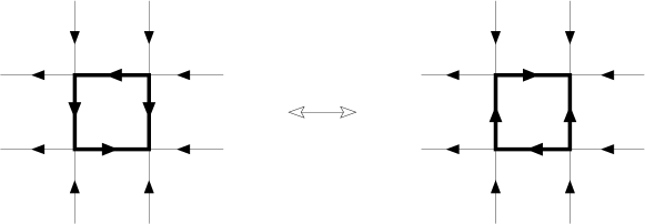
The kinetic term acts instead on a state by mapping it to a state (with coefficient ) such that configurations and differ by a single plaquette flip. Let us now define the set of local rearrangements needed to construct the reduced Hamiltonian fine-tuned to its RK point as the set of plaquette flips (i.e., reversal of the arrows on the edges of a plaquette) for all sites in the square lattice, and all the possible initial arrow orientations along the edges. An example of such plaquette rearrangements is given in Fig. 2.
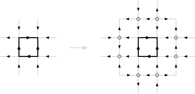
For reasons that will become clear in a moment, let us label these plaquette rearrangements by the set of all decorated and oriented plaquettes , defined by the site of their lower-left corner, by the orientations of the arrows along the edges of the plaquette, and by the orientations of the arrows on all eight dangling bonds that connect the sites of the plaquette to (nearest-neighboring) sites not belonging to the plaquette (see Fig. 2). We will also denote by the (unique) decorated and oriented plaquette that is obtained from by reversing all the four arrows along the edges of the plaquette. Notice that the number of elements in is times larger than the total number of simple oriented plaquettes (i.e., where only the directions of the arrows along the edges are specified). This redundancy, although superfluous for the kinetic operator alone, plays a crucial role when writing the potential energy term in the reduced form. We can now reinterpret Eq. (44) as
| (47a) | |||
| where [32] | |||
| (47b) | |||
| and | |||
| (47c) | |||
Here, is positive, is real-valued, [35, 36], and is the (unique) configuration that is obtained from after performing the plaquette flip . We stress that the role of the label in Eq. (47a) is two-fold. This label must specify the pair of classical configurations that “resonate” through a quantum tunneling process. This label must also carry the information needed to construct the difference between the classical configuration energies of the two classical configurations that “resonate”. For the eight-vortex model with no classical interactions between the vertices, is obtained by decorating the oriented plaquettes with the additional information on the orientations of the dangling bonds.
We have reinterpreted the quantum eight-vertex model fine-tuned to its RK point, introduced in Ref. [26], using the formalism presented in the past sections through Eq. (47a). It is now straightforward to generalize Eq. (47a), e.g., by adding interactions between the vertices as well as external fields. All this can easily be accommodated at the classical level, and thus at the quantum level as well, through a redefinition of , and possibly of . Notice in fact that the definition of decorated and oriented plaquettes given above, while sufficient to describe an applied field or chemical potential on the vertices (as in the original case by Ardonne et al.), needs to be modified if interactions between vertices are introduced. For example, in case of nearest-neighbor interactions one has to encode in the definition of a decorated and oriented loop the additional information about the types of nearest-neighboring vertices with respect to the ones belonging to the square plaquette, as illustrated in Fig. 3.
In the presence of interactions between vertices, the coupling constant can be interpreted as the inverse temperature of the classical problem defined by the GS. In addition to changing by extending the range of the decoration of an oriented plaquette, local rearrangements allowing moves in classical phase space different than single plaquette flips can be introduced. Any combination of these generalizations can change the zero-temperature phase diagram of the quantum model. Finally, we stress that the choice for the parameters can affect in a crucial way the classical stochastics (excitation spectrum) of the classical (quantum) system.
5.3 The quantum three-coloring model
So far we have illustrated how the formalism of the past sections reproduces quantum Hamiltonians fine-tuned to their RK points that have already been discussed in the literature, and how they can be generalized without spoiling the RK conditions (I-III). We devote the following discussion to the construction of a quantum Hamiltonian from an SMF decomposition whose classical counterpart exhibits dynamical glassiness.
Consider the classical three-coloring model on the honeycomb lattice with nearest-neighbor interactions [37, 38, 39, 40]. The model consists of classical degrees of freedom living on the nearest-neighbor bonds of a honeycomb lattice. Periodic boundary conditions are assumed. Any of these classical degrees of freedom can assume three different values or colors (say, A, B, and C). The system is also subjected to the hard constraint that each and every color emanates from any site of the honeycomb lattice. The classical configuration space is denoted by . To each coloring of the honeycomb lattice one can associate an Ising spin configuration with the Ising spins defined on the sites of the honeycomb lattice, according to the rule that a site is occupied by an up (down) Ising spin if the parity of the sequence of colors emanating from this site is even (odd) when encircling the site counter-clockwise, say. The classical energy of any coloring of the honeycomb lattice is taken to be the Heisenberg energy
| (48a) | |||
| Here, denotes an oriented pair of nearest-neighbor sites on the honeycomb lattice and is the spin stiffness. The classical partition function of the three-coloring model is then given by | |||
| (48b) | |||
The color constraint becomes the requirement that the sum over all the Ising spins around any elementary plaquette of the honeycomb lattice, a hexagon, be in the Ising spin representation. We refer the reader to Ref. [40] and references therein for a detailed analysis of the properties on the three-coloring model (48) in and out of thermal equilibrium. Suffice here to say that, in addition to the usual Ising ordered phases (Néel and ferromagnetic), there exists a large-temperature critical phase for in thermal equilibrium [41, 40]. This critical phase is expected to terminate in a first-order phase transition to the fully-magnetized ferromagnetic state for sufficiently positive . The ferromagnetic phase has very interesting properties out of thermal equilibrium. At and beyond this first order phase transition, the system encounters a dynamical obstruction to equilibration (classical dynamical glassiness) that gives origin to a supercooled liquid phase. The supercooled liquid phase freezes at a temperature into a polycrystallized phase with no interstitial liquid left. In view of the intimate connection between classical systems out of equilibrium and quantum Hamiltonians that admit SMF representations, it is then natural to ask if there is a signature of the classical dynamical glassiness in such quantum systems. The detailed answer to this question is beyond the scope of this paper. Below, we limit ourselves to the construction of an SMF decomposition of a quantum Hamiltonian that has the three-coloring model in thermal equilibrium emerging from its GS.
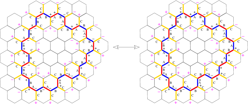
We define first the separable Hilbert space of the quantum problem as the span of the preferred, orthonormal basis states , labeled by the configurations of the three-coloring model. Since we are given the classical energy of any such configuration , we only need to construct the quantum kinetic energy to complete the definition of a quantum Hamiltonian that admits an SMF representation with the three-coloring model emerging from its GS. To this end, we note that the only classical updates allowed by the constraint involve exchanging the colors along closed, non-self-intersecting loops given by the sequence of two alternating colors starting at some site . In the spin language, any such update amounts to nothing but flipping all the spins along the loop, i.e., it can be thought of as being induced perturbatively by a transverse Ising field . Next, we need to construct the set of appropriately decorated loops so that: (i) they label all possible loop updates, and (ii) they carry enough information for the energy difference between two resonating configurations and to be written as a function . Both requirements are met when a decorated loop stands for: (1) The backbone structure of the loop, i.e., the sequence of sites visited by the loop. (2) The two-color sequence covering the loop. (3) The values of the spins that do not belong to the loop, but are connected to it by a single (dangling) bond. An example of such decorated loops is given in Fig. 4.
So far, the three-coloring model has been equipped with classical stochastics through Monte Carlo simulations using the Metropolis algorithm [40]. Correspondingly, we choose to implement the classical stochastics through a Master equation with transition matrix of the Metropolis form. We are now in the position to write the SMF decomposition of the quantum Hamiltonian whose GS normalization is nothing but the classical partition function of the classical three-coloring model,
| (49) |
The rescaling coefficient can be chosen at will. The loop energy is given by the integrability condition (14a): . The positive coefficient is chosen to obey the Metropolis condition (28a). The operators and are defined by their action on the basis states [32]
| (50) |
and
| (51) |
As it should be, the GS wavefunction in the preferred basis of the Hilbert space is
| (52) |
It is argued in Ref. [42] that a signature of dynamical glassiness can indeed be found in this quantum system when it is brought out of equilibrium through the local coupling to a heat bath.
We shall now refine what is meant above by locality. At the classical level in thermal equilibrium defined by Eqs. (48), locality is implemented by a pairwise interaction between the Ising spins that is short-ranged. Changing the range of the interaction leaves the backbone of a decorated loop unchanged while it does change its decoration. For example, if we modify (48a) by allowing a next-nearest neighbor Heisenberg interaction, we must then decorate a backbone with first and second nearest-neighbor dangling bonds. At the classical level out of equilibrium, i.e., at the quantum level, locality is implemented by the choice of the dependence on of . Since loops of all sizes participate to the classical stochastics (quantum dynamics) and since loops involve a number of Ising spins proportional to their perimeter, large loop updates (tunneling processes) must be penalized compared to small loop updates. Stochastic (dynamical) locality is thus achieved when decreases with the loop perimeter in an exponential fashion, say. We conclude that, in the Ising spin language, the (weak) coupling to the bath is local if it is between the and a bath of harmonic oscillators.
We close this discussion of the quantum three-coloring model that admits an SMF decomposition by illustrating how it can be thought of as a special point in parameter space of a more general quantum Hamiltonian, in the same preferred basis. Start from the quantum Ising model in a transverse field
| (53) |
defined on the honeycomb lattice. The large limit (i.e., ) restricts the physical Hilbert space to the one obtained by imposing on every elementary plaquette (hexagon) of the honeycomb lattice the hard constraint
| (54) |
In the same way as the model follows from the Hubbard model in the large limit, the quantum three-coloring Hamiltonian
| (55) |
follows from (53) when choosing the data properly [42]. The Hamiltonian (49) is another point in the parameter space specified by conditions (8) and conditions (14).
As a second example, we start from the medial lattice of the honeycomb lattice. This is the Kagome lattice obtained from the mid-points of the nearest-neighbor bonds of the honeycomb lattice. If we attach to any site of the Kagome lattice a quantum spin carrying angular momentum one, this gives a three-dimensional Hilbert space per site, and a global Hilbert space of dimension , with the total number of sites on the Kagome lattice. The three quantum numbers allowed for the component of the spin along the quantization (z) axis can be identified with the three colors , , and of the quantum three-coloring model. Next, we impose two constraints. First, we demand that the coarse-grained magnetization along the quantization axis vanishes. Here, the coarse-grained magnetization is defined locally on the honeycomb lattice by attaching to any site of the honeycomb lattice the arithmetic average over the spin quantum numbers along the quantization axis defined on the bonds meeting at this site. Second, we remove from any state that has all three spins with vanishing projection along the quantization axis when these three spins define a vertex of the honeycomb lattice. The combination of such two conditions on is equivalent to imposing the three-color constraint. Having defined the physical Hilbert space , we can then proceed as with the quantum Ising spin in a transverse magnetic field and identify a quantum Hamiltonian with nearest-neighbor spin-one interaction, say, with Hamiltonian (55). Closely related quantum spin-one models can be found in Ref. [43].
6 Conclusions
The study of quantum Hamiltonians that are of the Rokhsar-Kivelson type when represented in a preferred basis has proven fruitful in the study of quantum critical points. This is so because of an intimate relation between the matrix representations of these quantum Hamiltonians in preferred bases and some combinatorial problems of classical statistical physics.
We have shown in this paper that the examples of quantum Hamiltonians encountered this far, when fine-tuned to their RK points, belong to a broader class of real, symmetric, and irreducible matrices that are in one-to-one correspondence with matrices known in the mathematic literature as stochastic matrices. Any stochastic matrix can be used to define a Master equation of the matrix type that encodes the approach to thermal equilibrium of a classical system coupled to a heat bath. It is then natural to generalize the known examples of quantum Hamiltonians that are represented by matrices obeying the RK conditions (I-III) to any quantum Hamiltonian that admits a matrix representation in this broader class, that we dub the Stochastic Matrix Form (SMF) decomposition. Thus, some (not necessarily all) quantum phase transitions induced by tuning the coupling constants, say , , , etc., of a quantum Hamiltonian represented by a matrix which is SMF decomposable can be understood as classical phase transitions obtained by tuning the reduced inverse temperature , the chemical potential , the external field , etc., that enter a classical partition function as intensive thermal variables. This correspondence between the quantum GS and a classical partition function extends to the excitations of the quantum system and the relaxation modes of the classical system when the latter is properly coupled to a thermal bath.
The correspondence between a quantum Hamiltonian represented by a matrix which is SMF decomposable and Master equations of the Matrix type opens the intriguing possibility to find a signature in a quantum system for exotic properties of a stochastic classical system such as aging and dynamical glassiness. From a more practical point of view, this also suggests a classical Monte Carlo alternative to a quantum Monte Carlo simulation when probing numerically the excitation spectrum of a quantum system that allows for an SMF decomposition.
Finally, we have also proven that any quantum Hamiltonian, up to a shift of its eigenvalues, admits a continuous manifold of bases in which its representation is SMF decomposable. In this sense, the correspondence between a quantum Hamiltonian construed as an abstract operator acting on some separable Hilbert space and the stochastic dynamics describing the relaxation to thermal equilibrium of discrete classical statistical systems coupled to heat baths is one-to-continuously many.
We are indebted to Christopher Henley for a critical reading of our manuscript and for challenging us to explore the behavior of the SMF decomposition under a basis transformation.
References
- [1] R. H. Fowler and G. S. Rushbrooke, Trans. Faraday Soc. 33, 1272 (1937).
- [2] P. W. Kasteleyn, Physica (Amsterdam) 27, 1209 (1961) and J. Math. Phys. 4, 287 (1963).
- [3] M. E. Fisher, Phys. Rev. 124, 1664 (1961), J. Math. Phys. 4, 278 (1963), and J. Math. Phys. 7, 1776 (1966); M. E. Fisher and J. Stephenson, Phys. Rev. 132, 1411 (1963).
- [4] W. Thurston, Am. Math. Monthly 97, 757 (1990); Richard Kenyon, math-ph/0405052.
- [5] S. A. Kivelson, D. S. Rokhsar, and J. P. Sethna, Phys. Rev. B 35, 8865 (1987).
- [6] D. S. Rokhsar and S. A. Kivelson, Phys. Rev. Lett. 61, 2376 (1988).
- [7] S. Sachdev, Phys. Rev. B 40, 5204 (1989).
- [8] L. B. Ioffe and I. E. Larkin, Phys. Rev. B 40, 6941 (1989).
- [9] E. Fradkin and S. A. Kivelson, Mod. Phys. Lett. B 4, 225 (1990).
- [10] L. S. Levitov, Phys. Rev. Lett. 64, 92 (1990).
- [11] P. W. Leung, K. C. Chiu, and K. J. Runge, Phys. Rev. B 54, 12938 (1996).
- [12] C. L. Henley, J. Stat. Phys. 89, 483 (1997).
- [13] R. Moessner and S. L. Sondhi, Phys. Rev. Lett. 86, 1881 (2001).
- [14] X. G. Wen, Quantum Field Theory of Many-Body Systems (Oxford University Press, 2004).
- [15] R. Moessner, S. L. Sondhi, and P. Chandra, Phys. Rev. B 64, 144416 (2001).
- [16] R. Moessner, S. L. Sondhi, and E. Fradkin, Phys. Rev. B 65, 024504 (2001).
- [17] A. Ioselevich, D. A. Ivanov, and M. V. Feigelman, Phys. Rev. B 66, 174405 (2002).
- [18] P. Fendley, R. Moessner, and S. L. Sondhi, Phys. Rev. B 66, 214513 (2002).
- [19] G. Misguich, D. Serban, and V. Pasquier, Phys. Rev. Lett. 89, 137202 (2002) and Phys. Rev. B 67, 214413 (2003).
- [20] W. Krauth and R. Moessner, Phys. Rev. B 67, 064503 (2003).
- [21] R. Moessner and S. L. Sondhi, Phys. Rev. B 68, 054405 (2003).
- [22] D. A. Huse, W. Krauth, R. Moessner, and S. L. Sondhi, Phys. Rev. Lett. 91, 167004 (2003).
- [23] R. Moessner and S. L. Sondhi, Phys. Rev. B 68, 184512 (2003).
- [24] M. Hermele, M. P. A. Fisher, and L. Balents, Phys. Rev. B 69, 064404 (2004).
- [25] E. Fradkin, D. A. Huse, R. Moessner, V. Oganesyan, and S. L. Sondhi, Phys. Rev. B 69, 224415 (2004).
- [26] E. Ardonne, P. Fendley, and E. Fradkin, Annals of Physics (N.Y.) 310, 493 (2004).
- [27] C. L. Henley, J. Phys. C 16, S891 (2004).
- [28] The assumption that the Hilbert space is fully connected under the action of the time-evolution operator implies that the Hamiltonian matrix in the Hilbert space basis is irreducible. This requires in turn that no row or column in the matrix has less than one non-vanishing off-diagonal element. Since the Hamiltonian is symmetric, we immediately obtain a lower bound for , namely , and Eq. (3) holds.
- [29] See chapter 5 from “Matrices: Theory and Applications,” by D. Serre, Springer (New-York 2002). See also chapter A4.1 from “Quantum Field Theory and Critical Phenomena,” by J. Zinn-Justin, Oxford University Press (New-York 1996).
-
[30]
Notice that the operator acts on
the two-dimensional subspace of the Hilbert space given by the span of the
two basis states and . Hence,
can be represented by the
matrix
- [31] D. A. Ivanov, Phys. Rev. B 70, 094430 (2004).
- [32] For conciseness, the symbolic notation () means that the plaquette covering (decorated loop ) appears in configuration .
- [33] Provided we satisfy the conditions on the parameters , , and , which are: , , and integrable.
- [34] To be precise, there are cases when the change in energy, though local, cannot be written directly as a function of the simple rearrangements used in the noninteracting case (e.g., ). Typically however it is possible to redefine the rearrangements introducing an appropriate “decoration” that bears precisely the amount of information required to compute the energy difference . Examples of these decorated rearrangements will be given in Sections 5.2 and 5.3.
- [35] Notice that the simple additive nature of the energy in the eight-vertex model, where the Boltzmann weights are given by the product of the fugacities for the vertices, allows to satisfy trivially the integrability conditions on .
- [36] Notice the subtle difference between in Eq. (44c) and used here. The first counts the number of vertices of type that appear on plaquette in configuration , while the second counts the number of vertices of type that appear on the decorated and oriented plaquette . This is indeed the reason for the decoration of the oriented plaquettes: we want to be able to compute solely from the information contained in , without need of further knowledge of a configuration containing .
- [37] R. J. Baxter, J. Math. Phys. 11, 784 (1970).
- [38] P. Di Francesco and E. Guitter, Phys. Rev. E 50, 4418 (1994).
- [39] E. N. M. Cirillo, G. Gonnella, and A. Pelizzola, Phys. Rev. E 53, 1479 (1996).
- [40] C. Castelnovo, P. Pujol, and C. Chamon, Phys. Rev. B 69, 104529 (2004).
- [41] N. Read, reported in Kagome workshop (Jan. 1992), unpublished; J. Kondev and C. L. Henley, Nucl. Phys. B 464, 540 (1996); J. Kondev, J. de Gier, and B. Nienhuis, J. Phys. A 29, 6489 (1996).
- [42] C. Castelnovo, C. Chamon, C. Mudry, and P. Pujol, cond-mat/0410562.
- [43] Xiao-Gang Wen, Phys. Rev. B 68, 115413 (2003).