Inverse melting and inverse freezing: a spin model

Abstract

Systems of highly degenerate ordered or frozen state may exhibit inverse melting (reversible crystallization upon heating) or inverse freezing (reversible glass transition upon heating). This phenomena is reviewed, and a list of experimental demonstrations and theoretical models is presented. A simple spin model for inverse melting is introduced and solved analytically for infinite range, constant paramagnetic exchange interaction. The random exchange analogue of this model yields inverse freezing, as implied by the analytic solution based on the replica trick. The qualitative features of this system (generalized Blume-Capel spin model) are shown to resemble a large class of inverse melting phenomena. The appearance of inverse melting is related to an exact rescaling of one of the interaction parameters that measures the entropy of the system. For the case of almost degenerate spin states perturbative expansion is presented, and the first three terms correspond to the empiric formula for the Flory-Huggins $\chi$ parameter in the theory of polymer melts. Possible microscopic origin of this $\chi$ parameter and the limitations of the Flory-Huggins theory where the state degeneracy is associated with the different conformations of a single polymer or with the spatial structures of two interacting molecules are discussed.

I introduction

Inverse melting is a reversible transition between a liquid phase at low temperatures to a high temperature crystalline phase. This is an unusual and counter-intuitive phenomenon in which isobaric addition of heat causes liquids to crystallize, the reverse of the usual situation. For the opposite process, of melting a solid to a liquid, which is normally expected to produce cooling, in inverse melting heat is released as the solid melts. Clearly, inverse melting happens if, and only if, the so called ”ordered” phase (crystal) admits more entropy than the ”disordered” state; this may occur, e.g., if in the liquid phase some of the degrees of freedom of the elementary constituents are frozen, and melt in the crystalline phase.

Speaking about freezing and crystalization one should make the distinction between static phenomena, such as magnetization, degree of phase separation and crystalline order (Bragg peaks), and dynamical aspects, like the response functions, viscosity, ergodicity breakdown and so on. While the static features reflect the properties of the ”ground state” (lowest free energy state), the dynamics is dictated by the size of the potential barriers among different states. In the following, cases where the appearance of crystalline order is correlated with higher response functions will be mentioned, along with situations where ergodicity breaks down without the appearance of ordered structure, i.e., glass like transition. If such a transition occurs upon temperature increase we are speaking about ”inverse” glass transition, or inverse freezing, analogous to inverse melting.

Although rare, real substance examples of inverse melting phenomena have been found in a wide range of systems, as well as the formation, upon heating, of solid amorphous or glassy states. Since the transition that occurs on heating absorbs heat (as does normal melting), and the phase in equilibrium at higher temperatures has higher disorder or entropy, the crystalline or frozen amorphous phase are more disordered than the liquid phase. In each case, the greater order of average atomic positions in the crystal has to be offset by greater disorder in some other characteristic. Thus, all cases of inverse melting and inverse glass transition appear to involve a freezing of the center of mass location of the system constituents (molecules, polymers, flux lines). The loss of entropy due to this freezing is compensated by other microscopic degrees of freedom that are coupled to the center-of-mass position, where localization of the center of mass increases the amount of such excitations.

The aim of this paper is to survey the literature concerning the subject, to present and discuss an extremely simple spin model for inverse melting and inverse freezing, a model that has been recently presented by the authors schupper , and to extract some general features related to the phenomenon. The paper is organized as follows: in the second section we discuss the general characteristics of inverse melting and inverse glass transition and classify the different possible inverse melting scenarios. In section 3 we survey some real material examples from the literature, and ascribe them to the different classifications presented. Section 4 is devoted to modelling, where our simple spin model based on the well known Blume-Capel Blume model is presented along with previously discussed models. In section 5 we deal with the ordered version of our ”enriched” Blume-Capel model for inverse melting, and in the next section its disordered version and inverse freezing are discussed. Section 7 deals with the scaling properties of the model and we also show how its modification can be related to the temperature dependence of the interaction parameter of the Flory-Huggins like flory Huggins theories. Finally, some general conclusions and remarks are presented.

II Inverse melting and inverse freezing scenarios

II.1 Two types of first order inverse melting

Following Stillinger and Debenedetti, stillinger , we begin the discussion of inverse melting with the Clausius-Clapeyron equation that describes the slope of the melting curve in first order transition, e.g., the curve that describes the boundary between a crystal and a liquid in the T-P plane

$$\frac{dP}{dT}=\frac{S^{(2)}-S^{(1)}}{V^{(2)}-V^{(1)}}$$ (1)

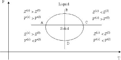
Figure 1: A sketch of the different melting curves in the T-P plane resulting from the Clausius-Clapeyron equation, including both types of inverse melting scenarios.

where $P(T)$ is the temperature dependent melting pressure, $S$ and $V$ denote the molar entropies and volumes, and the superscripts $2$ and $1$ denote the high and low temperature phases, respectively. Alternatively, these will be denoted by $l$ and $s$ for the liquid and solid phase. As noted first by Tammann Tammann , this thermodynamic equation offers schematically 4 different types of melting curves as shown in Figure (1) and will help to classify the known examples of first order transition scenarios. If the liquid-crystal transition is first order, at least one of $S^{(l)}-S^{(s)}$ and $V^{(l)}-V^{(s)}$ is non-zero at every point of the curve.

Let us identify the different regimes in this diagram. ’Normal’ melting involves an increase in both the entropy (the system absorbs latent heat) and the molar volume as the crystal becomes liquid. In that case, both $S^{(2)}-S^{(1)}$ and $V^{(2)}-V^{(1)}$ are positive, and therefore the slope of the curve is also positive. In figure (1) this is the portion of the curve between the points C and D. ”Anomalous”, or water-like, melting happens if the molar volume of the liquid is larger than that of the solid, $V^{(2)}-V^{(1)}$ becomes negative and the slope of the first order transition curve is also negative, i.e., the melting temperature decreases as pressure increases. The curve between the points B and C demonstrate this situation.

The left side of the circle, i.e., the intervals between A and B and between A and D are ranges of inverse melting, where isobaric heating takes the system from its liquid phase into the crystalline phase. If the transition involves latent heat, for any inverse melting situation $S^{(s)}-S^{(l)}>0$. For the interval from A to D $V^{(s)}-V^{(l)}$ is negative (the solid volume is smaller than the liquid) while the interval AB exhibits positive slope, since the solid is less dense than the liquid. Thus, there are two types of inverse melting, similar to the normal and anomalous usual melting. We shall denote the former case as inverse melting of type I, while the ”anomalous” case of larger molar volume in the ordered phase will be denoted as inverse melting of type II.

II.2 Order-disorder transition and response functions

As discussed in the introduction, the ”standard” solid-liquid transition involves both static (symmetry breakdown, Bragg peaks) and dynamic (diverging viscosity, rapid changes in the Young modulus, discontinuous susceptibility) aspects. In general, any of these may take place independently. For example, one may find an amorphous system with diverging (or at least very large) viscosity, like a glass. On the other hand, the order parameter may take a finite value but the ordered system is ”softer” than the disordered one, i.e., its response functions are larger, and therefore its viscosity smaller. In general we will speak about inverse melting when a liquid acquires crystalline structure upon heating, and about inverse freezing if the liquid becomes a glass (amorphus solid, with higher viscosity or an increase in other response functions, but no apparent order). An inverse solid-amorphous transition is another situation where an amorphous rigid material (similar to window glass) reversibly crystalizes as its temperature increases.

Although it is natural to associate an ”ordered” material with some sort of local structure, like a crystal, there are also other order parameters that one may define. In particular, phase separation of two liquids may be considered as a phase transition where the order parameter is associated with the local mixing of the fluids. Phase separation of polymer melts flory , for example, depends on the relation between the entropy gain of the mixture versus the energetic advantage of the separated state. It is well known polymerblends that some systems of polymer melts undergo phase separation when the temperature increases, a phenomena that, in some sense, is analogous to inverse melting (the ”ordered”, separated state is thermodynamically stable only above some temperature). In the Flory-Huggins flory Huggins theory of polymer melts, the free energy contains a temperature dependent interaction term. This implies that, to some extent, part of the internal entropy associated with the possible conformations of a single polymer is ”absorbed” into the interaction term to yield an effective, temperature-dependent interaction. The possible generalizations of this Flory-Huggins procedure for inverse melting is discussed in section VII.

II.3 Kinetics of inverse freezing

In any case of a first order transition between a liquid and a crystalline phase, the system freezes into a glassy state if the cooling is fast enough. The general kinetic description of this phenomenon is based on the distinction between the nucleation rate in a supercooled liquid (namely, the rate of creation of stable nuclei of the crystalline phase) and the growth rate of a crystal. Both processes are thermally activated and their rates admit maxima between the melting temperature and $T=0$. At the melting temperature, the bulk free energy associated with the two phases is the same, and there is no driving force towards nucleation, while as the temperature approaches zero, the kinetics of the system halts due to the divergence of viscosity [the rate of any thermally activated process depends on $exp(-\frac{\Delta E}{k_{B}T})$]. There is a difference, however, between the locations of these maxima, and in general one needs a lower temperature to get a reasonable nucleation rate, since there is a minimal size for a nucleus to be energetically favorable (the surface tension makes small nuclei thermodynamically unstable even below the melting temperature).

A good glass former liquid is associated, though, with diminishing overlap between the nucleation and the crystal growth zone, i.e., at temperatures just below the melting point there is no nucleation, while at lower temperatures, nucleation actually takes place but the crystal seeds could not grow as the viscosity diverges.

This picture yields a simple plausibility argument for inverse freezing, i.e., for a liquid that forms glass as it absorbs heat. Here, there is no decreasing kinetics as the temperature increases away from the melting point. Accordingly, any material that undergoes inverse melting is, generally, a very bad glass former. Unless some weird situation takes place, it is not plausible to get a glassy state of matter as a result of fast heating of a liquid. Accordingly, we suggest that inverse freezing appears, generically, only in systems with quenched disorder or, at least, if the glassy state is a true thermodynamic equilibrium state of the system.

III Examples of inverse melting and inverse freezing

Let us mention briefly some examples of systems displaying inverse melting which have been reported in the published literature, classify them as first or second order, type I or II, and attempt to explain their driving mechanisms shortly by the different sources of the entropy and volumes in the different phases involved. It should be stressed that the following list is by no means complete: a lot of literature is devoted to the glass-crystal transition under the name ”reentrent” reentrant , while the discovery of new systems is reported new .

Helium isotopes $He^{3}$ and $He^{4}$: Both isotopes display first order transition curves that qualitatively resemble the neighborhood of point D in figure (1), i.e. inverse melting of negative slope (type I) helium . For both isotopes the inverse melting happens at high pressures (about 25-30 bar) and, of course, at low temperature (less than 1K). There is, however, a difference in the character of the solid and the liquid phase. For $He^{4}$ a superfluid liquid becomes an hcp crystal upon heating (clearly the entropic gain here involves longitudinal phonons). For $He^{3}$, on the other hand, normal (i.e. non superfluid) liquid becomes a bcc crystal. This has to do with nuclear spin degrees of freedom that are relatively free to reorient independently in the crystal, thereby increasing its entropy relative to the liquid.

Metallic alloys: Inverse melting transformations have also been found in a number of binary alloys based on the early transition metals Ti, Nb, Zr, and Ta with later transition metals from groups V and VI. In inverse melting of alloys, a metastable supersaturated crystallic alloy transforms polymorphously to an amorphous state near the glass transition temperature upon heating metallicalloy . For example, metastable bcc $\beta$-TiCr phases with Cr contents between $40\%$ and $65\%$ which were prepared by mechanical alloying of elemental powder blends showed a polymorphous transformation of the bcc alloy into an amorphous phase. Furthermore, it was reported that this transition is reversible, such that the alloy can be switched back and forth between the amorphous and the bcc crystalline phase by application of alternating annealing steps at $800^{0}C$ and $600^{0}C$. From these results and also numerical thermodynamic calculations it was obtained that at those temperatures, a thermodynamic driving force must exist for the amorphization such that the free energy of the amorphous phase is lower than that of the bcc alloy for those configurations. The occurrence of inverse melting originates from a pronounced short-range ordering of the amorphous phase upon undercooling, which stabilizes the amorphous phase with respect to the bcc. Thus, although the crystal is much more topologically, long-range, ordered than the amorphous, the amorphous phase admits much more chemical short range order and therefore is of lower entropy.

Liquid crystals: An analogue to inverse melting, whose driving force is similar to the metallic alloys is provided by liquid crystals. It was shown that a first order boundary between smectic-A and nematic phases of 4-cyano-4’-octyloxybiphenyl (called 8OCB) looks very much like the portion A $\to$ B $\to$ C $\to$ D of Figure (1) Johari Cladis . The 8OCB liquid crystal molecule contains both a polar and a nonpolar part, as lipid bilayers. It consists of a flexible n-octane chain attached to a relatively rigid 4-cyano-biphenyloxy group. It was shown (by optical microscopy) that upon heating at a constant pressure the nematic phase transforms into a smectic-A phase, and on cooling again, it reversibly transforms back to the nematic phase. The nematic low temperature state possesses just molecular orientational order, while the smectic-A high temperature phase possesses both orientational and partial translational order. Long range attractive electrostatic forces stabilize layering, while the short range repulsive interactions stabilize the nematic phase at low temperatures. Thus, in this material many internal degrees of freedom are coupled to the orientational and positional order to produce an inverse melting analogue. In addition, ”re-entrant” nematic $\longleftrightarrow$ smectic-A transformations were observed in binary mixtures of analogous molecules. The thermodynamics of the binary mixtures may involve also an alloy-like chemical short range ordering in the nematic phase. It was proposed Johari , that tight but mobile configurations of associated molecular pairs reduce the entropy of that phase.

Ferroelectricity in Rochelle Salt Rochelle salt ($NaKC_{4}H_{4}O_{6}\cdot 4H_{2}O$, double sodium potassium tartrate tetrahydrate) is a ferroelectric material exhibiting two Curie points: one at $-18^{0}C$ and the other at $+24^{0}C$ rochelle . This material is ferroelectric with a monoclinic point group 2 and, in its non-ferroelectric region, its structure belongs to the orthorhombic point group 222. The higher Curie point is similar to regular ferroelectric transition, however, the lower point - the point where the spontaneous polarization is lost, and the system becomes paraelectric (disordered) - is not trivial, since the crystalline structure above the upper Curie point and below the lower Curie point are the same. This time the inverted transition is second order in type. Both the higher and the lower Curie point go up in temperature at higher pressure, i.e., $dP/dT>0$. In the next section the theoretical explanations for this behavior are presented.

Water The liquid-liquid transition theory for polyamorphous materials, i.e. materials that can have more than one amorphous form, predicts an inverse freezing transition even for the most known liquid, water. In the hypothesized phase diagram presented in stanley , below a second critical point with coordinates $T=220K$ and $P=100MPa$, the liquid phase separates into two distinct liquid phases: a low density liquid (LDL) phase at low pressures and a high density liquid (HDL) at high pressures. Between these points water is a fluctuating mixture of molecules whose local structures resemble the two phases, LDL and HDL. The small region between $100MPa$ and $150MPa$ and temperatures between $-50^{0}C$ to $-100^{0}C$ exhibits a range of inverse melting where the low density amorphous becomes a low density liquid upon cooling. Although the region of this hypothetic inverse freezing scenario is not accessible experimentally, it is interesting to note the possibility of an inverse transition even is the most familiar and important liquid on earth.

Magnetic films An inverse transition effect is also found in ultra-thin Fe films that are magnetized perpendicular to the film plane Portmann . The magnetization of these films is striped domains with opposite perpendicular magnetization. From scanning electron microscopy it was found that when the temperature is increased, the low temperature stripe domain structure transforms into a more symmetric, labyrinthine structure. However, at even higher temperatures and before the loss of magnetic order, a re-occurrence of the less symmetric stripe phase is found. The mechanism driving this transition is topological defects such as dislocations and disclinations. More specifically knee-bend and bridge instabilities lead to the straightening of the labyrinthine pattern when the temperature is increased. Thus the increase in topological disorder drives the transition.

Vortex lines in disordered high temperature superconductor: First order, type II transition from glassy to a crystalline state was discovered in the lattice formed by magnetic flux lines in a high temperature superconductor $Bi_{2}Sr_{2}CaCu_{2}O_{8}$ (BSCCO) pinning . The ordered hexagonal lattice has larger entropy than the low temperature disordered phase. The explanation suggested is that the transition from the lattice to the glass phase is driven by pinning of the flux lines to impurities in the crystal at low temperatures. The competition between thermal fluctuations and pinning disorder leads to inverse melting near the critical point. In this system, however, the intensive order parameter (bulk magnetization) is lower in the crystalline phase, and the response functions are higher, i.e., the disordered phase is stiffer than the ordered phase.

”Cold denaturation” of proteins: Most of the proteins denaturate, i.e., lose their biologically active, native state, at high temperatures. Since a protein is a complex object with many degrees of freedom, its denaturation transition resembles a ”true” first order transition in an infinite system Proteins . In contrast with the ”regular” denaturation upon heating, the protein ribonuclease A displays a reversible ”inverse denaturation” upon cooling (type II inverse melting) at high pressure (about 4kbarr). This phenomenon may be explained on the basis of the internal structure of the protein itself, as secondary or higher order structures are lost upon denaturation. A different explanation which has been proposed is the loss of ”low density water” as the cause for cold denaturation ColdDenat , this has been modelled and found in agreement with the experimental data. In addition to the study of ribonuclease A, cold denaturation at very high pressures has also been observed in other biological systems Biology .

Colloidal systems- PMM1 sticky spheres: A simple model system which was studied both theoretically and experimentally is a collection of hard spheres in a given volume. Hard sphere particles are increasingly caged by their neighbors as the density increases and at a critical density, the system becomes non-ergodic or glassy. The glass transition in that case depends only on the filling fraction of the system and is independent of temperature, as the thermal energy is negligible compared with the repulsion. The addition of short-range inter-particle attraction (stickiness) introduces new energy scale, and a corresponding temperature, into the problem. It was shown that, as temperature decreases, the attraction first ’melts’ the ”hard sphere” glass, thus causing an inverse freezing transition, and then, upon further decrease of the temperature, a second, qualitatively different, glassy state is formed due to the attractive interactions. Experimentally Pham2 the system consisted of a colloidal system of sterically stabilized polymethylmethacrylate (PMMA) particles, dispersed in cis-decalin, with short range attraction induced by adding a non-adsorbing polymer, polystyrene. The polymer is excluded from the region between the surfaces of two nearby particles, thus leading to an excess osmotic pressure attracting the particles together. From the behavior of the samples, it was found that the line of structural arrest at the high-density end of the phase diagram has a re-entrant phase. This has also been observed by MCT calculations Pham , MD simulations, and light scattering experiments which all suggest that the qualitatively distinct kinds of glasses are dominated by repulsion and attraction, respectively.

Polymeric systems:

(a) Poly (4-Methylpentene-1): A different inverse melting material is the polymeric substance poly(4-methylpentene-1) denoted more simply as P4MP1greer . This is a semi-crystalline one component polymeric system having a crystalline component of nearly $60\%$. Below the glass transition temperature (at around room temperature and atmospheric pressure), the crystal density of the polymer is lower than the amorphous phase. Therefore, on compression, the initially crystalline tetragonal phase loses order and becomes amorphous above a threshold value of 2kbar. This transformation is exothermic in nature, thus suggesting that the amorphous phase has lower entropy than the crystalline tetragonal phase. Indeed, a disordering on cooling of the crystalline phase, that is, inverse melting and crystallization on heating were observed. These structural changes have also been confirmed by other experimental methods. It was observed that the melting curve in the T-P plane possesses a maximum of the type shown in figure (1) by point B and its neighborhood, i.e. the slope of the inverse melting curve is positive (Type II). This ’solid state amorphization’ is in agreement with the unusual density relationship below the glass transition temperature of the polymer. The mechanism for the inverted transition is the larger amount of conformations of backbone and side-groups of the polymer in the crystal, which are due to its more open structure, and this contributes to its overall higher entropy.

(b) Methyl Cellulose: An interesting example in polymeric systems for inverse glass transition is the reversible thermogelation of Methyl Cellulose solution in water Chevillard . When a (soft and transparent) solution of Methyl Cellulose is heated (above $55^{\circ}$C, for a 5 gr/liter solution) it turns into a white, turbid and mechanically strong gel. This transition is reversible, and upon subsequent cooling, the polymer is redissolved again. In its high temperature phase, Methyl Cellulose gel exhibits, like many other gels gel , glassy features. In this case, the folded conformation is favored energetically while its unfolded conformation is favored entropically [See figure (2)]. The entropy growth of the open conformation may be related to the number of possible microscopic configurations of the polymer itself, but it may be attributed also to the spatial arrangement of the water molecules in its vicinity, similar to the process suggested before for protein denaturation. The mechanism proposed also for other systems displaying inverse transitions due to the hydrophobic effect hydrophob is as follows: In the liquid state the water molecules are kept in a highly constrained ’cage like’ structures formed by the hydrophobic constituents which move around in the solution. However, as the gel is formed, and the hydrophobic segments cluster together to form cross-links, these cages are opened, and the water molecules move freely around the network. As a consequence, the number of possible configurations and the entropy of the water molecules (which highly determines the entropy of the whole system consisting of $99\%$ water) is low in the liquid phase and increases when hydrophobic aggregates cluster together and form a gel haque . The main cause for inverse glass transition is that the ”open” high entropy conformations of the polymer are also the interacting structures, as they allow for the formation of hydrophobic links with other polymers in the solution, a process that leads to gelation.

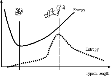
Figure 2: A sketch of the energy and entropy dependence on the linear size of a Methyl Cellulose polymer in water. The folded conformation costs less energy due to more favorable interactions between hydrophobic sequences along a single chain, but are less entropic as water molecules have less freedom around the hydrophobic constituents of the chain. The unfolded conformation admits much more microscopic configurations. The interaction with other polymers in the solution is suppressed in the folded state and therefore it constitutes the liquid.

(c) Other Polymers: Aqueous solutions of the triblock copolymer PEO-PPO-PEO (PPO - polypropylene oxide, PEO - polyethylene oxide) also show inverse melting behaviorMortensen . Similar to methyl Cellulose, due to the entropic mechanism, the PPO block is hydrophobic at high temperatures and hydrophilic at low temperatures. Above a certain concentration and a specific temperature, the Gaussian chains of these polymers form micelles. At even higher temperatures it is found that the micellar liquid transforms into a stable cubic (bcc) crystal. In contrast to the methyl Cellulose, the transition is to an ordered solid since the hydrophobic sequences are deposited at ordered positions along the chain. The entropy change due to crystallization may be small compared to the entropy change of molecular origin and this is the assumed mechanism for the inverse melting transition.

Table 1: A summary of the different known physical systems exhibiting inverse melting and the transition characteristics.

IV Theoretical Modelling

As mentioned above, the Flory-Huggins theory of phase separation in polymer melts may yield phase separation as temperature increases. In this theory, however, a temperature dependent interaction is included. In this section we try to review several ”first principle” models that exist in the literature. In these models, the ground state energy and the excitation spectrum are temperature independent, and the inverse transition is attained by applying the thermodynamic consideration to the given spectrum.

Rochelle salt: Perhaps the first theoretical considerations that dealt with inverse melting appeared in the context of the two Curie points for the ferroelectric phase of Rochelle salt mitsui . The model may be presented in a form of ”quantum” pseudo-spin model, where the Hamiltonian is non-diagonal in the $z$ direction blinc and two sublattices are defined with different local field and interactions. The combined effect of thermal and quantum tunneling dominate the system in some temperature range to yield a finite magnetization in the $z$ direction.

Random heteropolymer in a disordered medium: In a recent model presented by Shakhnovich et. al. randompoly , a random heteropolymer in a disordered medium is considered. Here, as in the flux line crystallization problem pinning , the low energy, low entropy state of the polymer involves pinning by quenched randomness that corresponds to a wandering exponent larger than the $1/2$ value associated with thermal wandering and crystallization is avoided. At larger temperatures the impurity pinning may be neglected and the thermally wandering polymers are free to form a structure based on their mutual interactions. In case of random heteropolymers, this structure is glassy, as opposed to the crystalline structure obtained in the flux line case.

Extended gaussian core model: In a recent work by Feeney, Debenedetti and Stillinger feeney , an extension of the Gaussian core model has been presented as a model that includes first order inverse melting transitions. The particles of this model are point particles that interact via a Gaussian repulsive potential, and in the extended model any single particle may be in one of two internal states, where the ground state is non degenerate and the excited state admits high degeneracy. If the interaction range of the excited states is shorter than the interaction range of a particle in the ground state, the effective density of particles decreases as temperature is increased. This leads to a type II (water like) inverse melting scenario, since the molar volume of the solid is larger than that of the liquid. On the other hand, if in the extended model the interaction range for the ground state is shorter, heating induces larger effective density that yields type I inverse melting scenario.

Extended Blume-Capel model: The spin model presented below contains the basic ingredients of the extended gaussian core model in a spin system. Its advantage relays on the simplicity of modeling and solutions, and it gives a unifying framework to analyze both inverse melting and inverse freezing of type I, type II, first and second order. Although this model is not directly related to any of the systems presented above, it may yield various general insights into the inverse transitions as shown in the next sections.

V Spin model for inverse melting: the ordered case

V.1 a model for inverse melting of type I

It has already been explained that, in order for inverse melting of type I to occur, the more frozen, interacting, state has to be of higher entropy, i.e. to have more internal configurations, than the liquid noninteracting state. In order to model this phenomenon in a most simple way one should look for the simplest model that incorporates all these features. Here we use a modified version of the Blume-Capel model Blume . The fundamental constituents are spin one particles, and there are two competing interactions: an exchange interaction that lowers the energy of the $\pm 1$ (interacting) states, and a ”lattice field” that favors the ”zero” (noninteracting) state. For $N$ interacting spins the Blume-Capel (BC) Hamiltonian takes the form:

$$H=-J\sum_{<i,j>}S_{i}S_{j}+D\sum_{i=1}^{N}S_{i}^{2}-h\sum_{i=1}^{N}S_{i}$$ (2)

where the spin variables are allowed to assume the values $S_{i}=0,\pm 1$. The summation over $<i,j>$ is over any interacting pair once and $h$ is the magnetic field applied. The magnetic field term that breaks the up down symmetry of the spins has no direct relevance to the inverse melting and is included here only for completeness of the discussion and for susceptibility calculations. Nevertheless, the phase diagrams below, will be plotted for $h=0$.

For positive $D$ the noninteracting state of a single spin is lowered in energy than the interacting state. For $D>qJ$ (where $q$ is the number of interacting particles, or ”nearest neighbors”, of the model), the ground state of the Hamiltonian is the ”folded” state, where all spins are zero, i.e., the system is in its noninteracting phase. For $D<qJ$ it is favorable for the system to be in its interacting phase, and at the ground state all spins are either at the $+1$ or at the $-1$ states. At zero temperature this implies a transition, upon increasing $D$, from the ferromagnetic state to the paramagnetic one, and spontaneous breakdown of the up-down symmetry in the interacting phase. Thus, this model already includes one basic ingredient of the inverse melting scheme, namely, the energetic preference of the non interacting state.

In order to explain the second constituent essential for our model let us use the Methyl Cellulose analogy [see Figure (2)] as an example. If the zero spin state of the BC model represents schematically the compact non-interacting polymer coil, the stretched polymer (interacting with its neighbors) is represented by spin $\pm 1$. Clearly there are many possible spatial configurations in which two polymers may attach to each other, and correspondingly many degenerate, or almost degenerate, frozen configurations of the gel; in our schematic model this is represented by the degeneracy between plus and minus states.

The new ingredient that should be added to the classical BC model in order to yield inverse melting is the entropic advantage of the interacting states. As a first approximation let the $0$ spin state to be k-fold degenerate, and the $\pm 1$ states to be are l-fold degenerate where $r=l/k\geq 1$ is the degeneracy ratio that dictates the entropic advantage. It turns out that all the results presented here are independent of the absolute degeneracies $k$ and $l$, and depend only on their ratio $r$. The parameter $r$ represents, of course, the more configurations available for a polymer in its opened (interacting) states relative to the number of configurations it can obtain in the closed (noninteracting) coil.

The Blume-Capel model, as well as its modification presented here may be easily solved in its infinite range limit, i.e., where there is no spatial structure and any pair of spins interact with each other. In order to keep the effective field finite one replaces the exchange factor in the Hamiltonian $J$ by $J/N$. Using standard gaussian integral techniques one finds an expression for the free energy per spin in the infinite range limit:

$$\beta f\equiv\beta F/N=\frac{\beta JM^{2}}{2}-ln\{1+2\ r\ cosh[\beta(JM+h)]e^{-\beta D}\}$$ (3)

where $M$ is the order parameter of the system (magnetization per spin), $M\equiv\langle\frac{1}{N}\sum_{i=1}^{N}S_{i}\rangle$. The phase transition curves are obtained numerically by solving for the minimum of Eq. (3) with respect to $M$, namely, the equation

$$M=\frac{2r\sinh[\beta(JM+h)]}{e^{\beta D}+2r\cosh[\beta(JM+h)]}$$ (4)

should be solved self consistently.

Figure 3: Phase diagram and spinodal lines for the ordered model Eq. (3) in the $D-T$ plane for $r=1$ (Blume-Capel model, inset) and for $r=6$. The value of $r=6$ has been chosen in order for the effect to be more pronounced, but inverse melting is seen as soon as $r>1$. As mentioned in the text, the effect of introducing a magnetic field will not be considered and all phase diagrams will be plotted for $h=0$.

Scaling the temperature and $D$ with the interaction strength $J$, the phase diagram is shown in Figure (3). In the inset, results are presented for the original Blume-Capel model (i.e., the $r=1$ case): the line AB is a second order regular transition line, above it is a paramagnetic ($M=0$) phase and below it the system is Ferromagnetic ($M\neq 0$). Below the tricritical point (B) the phase transition is first order, and the three lines plotted are: the spinodal line of the ferromagnetic phase BE (above this line the $M\neq 0$ solution ceases to exist), the spinodal line of the paramagnetic phase BC (below this line $M=0$ is not a minimum of the free energy) and the first order transition line BD. Along BD the free energy of the paramagnetic phase is equal to that of the ferromagnetic state. Clearly, the Blume-Capel model displays no inverse melting: an increase of the temperature induces smaller order parameter.

The situation is different as $r$ increases, as emphasized by the main part of Figure (3). The same phase diagram is presented, but now $r=6$, so the interacting states have larger entropy. The ferromagnetic phase now covers a larger area of the phase diagram, a fact that reflects its entropic advantage. The tricritical point is shifted to the left, relative to the point of infinite slope, leaving a region of second order inverse melting, and the orientation of the BD line also changes, establishing the possibility of first and second order inverse melting. Note that the $r=6$ transition lines converge to the $r=1$ lines as $T\to 0$, since the entropy has no effect on the free energy at that limit.

The value of $r=6$ was chosen only for illustration. In fact, as soon as $r$ gets larger than 1, inverse melting of first order is observed. For $r=1$, i.e. the original Blume-Capel model, the tricritical point is placed a bit higher then the point of infinite slope and the BD line curves to the right. However, as $r$ increases a bit, a small portion of the BD line obtains negative curvature, thus inserting a small region of first order inverse melting. However, the general trend of the first order transition line BD is still to the right. The tricritical point begins to move downwards through the AB line and continues to do so on a further increase of $r$. It crosses the point of infinite slope for $r\sim 1.1204$ and thus for larger values of $r$, first and second order regions of inverse melting occur as the tricritical point continues to move downwards on the melting curve to below the point of infinite slope. All in all, it seems that the original Blume-Capel, i.e. for $r=1$ is exactly ”marginal” in the sense of inverse melting.

To allow qualitative comparison of our cartoon model with experimental results, the appropriate parameters should be identified. There are three parameters in the model as it stands: $D$ represents the energetic advantage of the noninteracting state, $r$ (if larger than 1) is the entropic gain of the interacting state, and $J$ is the strength of the interaction. In most of the physical systems that display inverse melting, the controlled external parameter is the strength of the interaction: pressure (for $He^{3}$ and $He^{4}$) or concentration of the interacting objects (for polymeric and colloidal systems and Rochelle salt - Ammonium Rochelle salt mixtures). As long as the only effect of the pressure is to increase the strength of the effective interaction among constituents, it may be modelled by changing $J$. The resulting phase diagram should be compared, though, with the $T-J$ plot of our model presented in Figure (4) and shows type I, i.e. negative slope, inverse melting. The decrease of the transition temperature with the increase of interaction strength (pressure) is physically intuitive, as larger interaction favors energetically the ferromagnetic phase. As discussed previously, the slope of the first order transition line in the temperature-pressure plane is required by the corresponding Clausius-Clapeyron equation (1).

Inverse melting obtained by this model is type I, $V^{(s)}<V^{(l)}$, and one expects a negative slope of the transition line as was also shown in portion AD of figure (1). In real magnetic or electric system the intensive-extensive pairs [magnetic field-magnetization ($\textbf{H}\cdot d\textbf{M}$) or electric field-polarization ($\textbf{E}\cdot d\textbf{P}$)], appear in the free energy function with inverse sign relative to $PdV$. If the order parameter vanishes, or takes smaller values, in the ”liquid” (disordered) phase, this implies also negative slope of the first order transition line in the temperature-external field plane.

Figure 4: Phase diagram and spinodal lines for the ordered model Eq. (3) in the $T-J(P)$ plane for $r=6$. First and second order inverse melting of the first type are observed, i.e. the slope of the curve is negative.

V.2 a model for inverse melting of type II

The modelling of type II inverse melting, where the volume of the liquid is lower than that of the crystal is possible by slight modification of the Hamiltonian. Following ColdDenat we add an additional energetic ’cost’ to the interacting states of the hamiltonian, thereby reducing the net gain in the free energy obtained for a large $r$. Thus the frozen interacting state is also of higher volume than the noninteracting one and its energy increases. The Hamiltonian becomes

$$H=-J\sum_{<i,j>}S_{i}S_{j}+D\sum_{i=1}^{N}S_{i}^{2}+P\delta V\sum_{<i,j>}S_{i}S_{j},$$ (5)

where $\delta V$ is the access volume of the ”open”, interacting configurations. Plotting the locus of the phase transition, this time as a function of pressure, yields the phase diagram shown in figure (5). The slope of the $P(T)$ diagram is shown positive. This is analogous to raising the energetic cost of the interacting state to a state where $J_{eff}=J-P\delta V$. Therefore, for higher values of $P$, higher temperatures are needed to induce the inverted transition.

Figure 5: Phase diagram and spinodal lines for the ordered model Eq. (5) of the second type in the $T-P$ plane for $r=6$. The slope of the inverse melting curve is positive this time.

V.3 Response functions

To complete the picture let us calculate the values of some thermodynamic quantities that characterize the transitions in the first version of the model. The heat capacity, given by

$$C_{H}=2rk_{B}\beta^{2}\exp(\beta D)\cdot\frac{2rJ^{2}M^{2}-2DJM\sinh[\beta(JM+h)]+(D^{2}+J^{2}M^{2})\cosh[\beta(JM+h)]}{\left[\exp(\beta D)+2r\cosh[\beta(JM+h)]\right]^{2}}$$ (6)

In figure (6) the heat capacity as a function of temperature is shown for different values of $D/J$ (i.e., along vertical sections of the phase diagram (3). For small $D/J$, where there is no inverted phase transition (demonstrated in the figure by $D/J=0.3$), the heat capacity shows only a monotonic increase to a maximum followed by a decrease as expected by thermal changes. In the point of second order (normal) melting, the slope changes suddenly. Since the model is globally coupled, there is no meaning to the correlation length and domain size and therefore, the diverging heat capacity associated with second order transitions is avoided. For higher values of $D/J$ (shown for $D/J=0.8$), as the first order inverse transition sets in, there is a discontinuity of the heat capacity. Following this is an increase, then a decrease, of the heat capacity with the temperature and again an abrupt change of the slope when the second order melting occurs. Second order inverse melting, (as obtained for $D/J=1.2$) also shows an abrupt change in the derivative of the specific heat at the transitions (not easily seen in the figure at $T=0.5$ and $T=0.75$). For higher values of $D/J$ there are no phase transitions so the heat capacity is a monotonic function.

Figure 6: Heat capacity as a function of the scaled temperature $T/J$ for the ordered model, Eq. (3), for different values of $D/J$. First order inverse melting shows a jumps in the heat capacity while second order transitions show a discontinuity in the derivative of the heat capacity.

The susceptibility as a function of temperature is given by

$$\chi=\left(\frac{2r\sinh^{2}(\beta JM)^{2}}{\beta M^{2}[2r+\exp(\beta D)\cosh(\beta JM)]}-J\right)^{-1}$$ (7)

and several vertical cuts are shown in Figure (7). First order inverse melting yields a small discontinuity in the susceptibility as seen more clearly in the inset for $D/J=0.8$. However, all second order transitions in the system, including the inverted ones give diverging values of the susceptibility at the transitions, as expected.

Figure 7: Susceptibility as a function of the scaled temperature $T/J$ for the ordered model, Eq. (3), for different values of $D/J$. First order inverse melting shows a discontinuity in the susceptibility while second order transitions show divergences.

VI spin model for inverse freezing

VI.1 Model system and the replica trick

As already explained in the introduction, inverse freezing is the (reversible) appearance of glassy features in a system upon raising the temperature. This may be incorporated in our spin model by introducing random coupling $J_{ij}$, as in the standard spin-glass models binder . The random-exchange generalization of the Hamiltonian (2) is:

$$H=\sum_{<i,j>}J_{ij}S_{i}S_{j}+D\sum_{i=1}^{N}S_{i}^{2}-h\sum_{i=1}^{N}S_{i}$$ (8)

where the exchange interaction between the $i$ and the $j$ spin is taken at random from some predetermined distribution. Following the paradigmatic Sherrington-Kirkpatrick (SK) analysis binder of the infinite range spin glass, we assume gaussian distribution of the exchange term with zero mean:

$$P(J_{ij})=\sqrt{\frac{N}{2\pi J^{2}}}\exp-[\frac{N(J_{ij}-\frac{J_{0}}{N})^{2}}{2J^{2}}],$$ (9)

where $\frac{J_{0}}{N}$ is the mean of the distribution and $\frac{J}{\sqrt{N}}$ is its width. The replica trick is then implemented to get the free energy at the large $N$ limit.

The case $r=1$, namely the random exchange version of the Blume-Capel model, was first introduced and discussed by Ghatak and Sherrington (GS) Ghatak who used symmetric replica to obtain the relevant phase diagram. The GS solution seems to display inverse freezing very pronouncedly even for the $r=1$ case, but more detailed analysis by da Costa et. al. Costa revealed errors in the numerical stability analysis of GS. They discovered that the glass order-parameter takes nonzero values (with a variety of stability features) in the area below the GS transition line, and the temperature dependence is monotonic. In their corrected solution only a very tiny ”inverse melting” region exists. Recently, the full replica symmetry breaking analysis has been implemented for the GS model crisanti , and the results admit no inverse glass transition. Here we present a replica symmetric analysis of the same hamiltonian where the interacting states are highly degenerate, i.e., $r>1$. Following Costa , we obtain the phase transition and the spinodal lines, and the results support, again, both first and second order inverse glass transition. The generalization of the replica symmetry breaking technique to both the Blume-Capel and the Blume-Emery-Griffith models has been carried out by Arenzon .

The replica technique Edwards relies on the identity

$$\overline{ln[Z]}=lim_{n\rightarrow 0}\frac{1}{n}(\overline{Z^{n}}-1),$$ (10)

where $Z$ is the partition function of the system and $Z^{n}$ is interpreted as the partition function of an n-fold replicated system $S_{i}\rightarrow S_{ia},a=1...n$. The average free energy per spin may be computed using

$$\beta f=-lim_{n\rightarrow 0}\frac{1}{Nn}(\overline{Z^{n}}-1).$$ (11)

The disorder average is taken for $Z^{n}$ using the Gaussian distribution (9) and yields:

$$\overline{Z^{n}}=Tr_{\{S_{i,a}\}}\exp\left[\frac{\beta^{2}J^{2}}{2N}\sum_{a>b}\left(\sum_{i}S_{ia}S_{ib}\right)^{2}+\frac{\beta^{2}J^{2}}{4N}\sum_{a}\left(\sum_{i}S_{ia}^{2}\right)^{2}-\beta D\sum_{a}\sum_{i}S_{ia}^{2}\right.$$ (12)

$$\left.+\frac{\beta J_{0}}{2N}\sum_{a}\left(\sum_{i}S_{ia}\right)^{2}+\beta h\sum_{a}\sum_{i}S_{ia}\right]$$

where $a,b=1...n$ are the replica indices. Implementing the Hubbard-Stratanovitch identity yields the free energy per spin:

$$-\beta f=-\beta\frac{F}{N}=\lim_{n\rightarrow 0}\frac{1}{n}\{-\frac{\beta^{2}J^{2}}{2}\sum_{a>b}q_{ab}^{2}\ -\frac{\beta^{2}J^{2}}{4}\sum_{a}q_{aa}^{2}-\frac{\beta J_{0}}{2}\sum_{a}M_{a}^{2}+lnTre^{\hat{L}}\}$$ (13)

where

$$\hat{L}=\beta^{2}J^{2}\sum_{a>b}q_{ab}S_{a}S_{b}+\frac{\beta^{2}J^{2}}{2}\sum_{a}q_{aa}S_{a}^{2}-\beta D\sum_{a}S_{a}^{2}+\beta J_{0}\sum_{a}M_{a}S_{a}+\beta h\sum_{a}S_{a}$$ (14)

with $M_{a}$ the magnetization in each replica and $q_{aa}$, $q_{ab}$, are the diagonal and the off diagonal entries of the ”order parameter matrix”. All these quantities are given self-consistently by the saddle-point conditions:

$$M_{a}=\langle{S_{a}}\rangle\qquad q_{aa}=\langle{S_{a}^{2}}\rangle\qquad q_{ab}=\langle{S_{a}S_{b}}\rangle$$ (15)

as $\langle...\rangle$ stands for thermal average over the effective hamiltonian $\hat{L}$.

VI.2 replica symmetric solution

In order to solve this model it is necessary to make assumptions on the order parameter matrix elements $q_{ab}$. In order to get a general qualitative picture of the phase diagram of the system we first make the simplest ansatz, which is symmetry with respect to permutations of any pair of the replicas: $m_{a}=m,q_{aa}=p,\ \ \forall a$, and $q_{ab}=q,\ \ \forall a\neq b$. Using this replica symmetric assumption one obtains

$$-\beta f_{rs}=\frac{\beta^{2}J^{2}}{4}(q^{2}-p^{2})-\frac{\beta J_{0}}{2}M^{2}+\frac{1}{\sqrt{2\pi}}\int_{-\infty}^{\infty}dz\exp(-\frac{z^{2}}{2})ln[1+2\ r\ e^{\gamma}\cosh(\beta\tilde{H}(z))]$$ (16)

with

$$\tilde{H}(z)=J\sqrt{q}z+J_{0}M+h$$ (17)

and

$$\gamma=\frac{\beta^{2}J^{2}}{2}(p-q)-\beta D$$ (18)

Extremizing the free energy with respect to $q$, $p$ and $M$ one gets the following set of coupled equations:

$$q=\int_{-\infty}^{\infty}\frac{dz\ exp(-\frac{z^{2}}{2})}{\sqrt{2\pi}}\left[\frac{2re^{\gamma}\sinh(\beta\tilde{H}(z))}{1+2re^{\gamma}\cosh(\beta\tilde{H}(z))}\right]^{2}$$ (19)

$$p=\int_{-\infty}^{\infty}\frac{dz\ exp(-\frac{z^{2}}{2})}{\sqrt{2\pi}}\frac{2re^{\gamma}\cosh(\beta\tilde{H}(z))}{1+2re^{\gamma}\cosh(\beta\tilde{H}(z))}$$ (20)

$$M=\int_{-\infty}^{\infty}\frac{dz\ exp(-\frac{z^{2}}{2})}{\sqrt{2\pi}}\frac{2re^{\gamma}\sinh(\beta\tilde{H}(z))}{1+2re^{\gamma}\cosh(\beta\tilde{H}(z))}$$ (21)

The coupled equations (19),(20) and (21) are solved numerically (with the possibility of multiple solutions if more than one stable state exists). In the limit where $h\rightarrow 0$ and $J_{0}\rightarrow 0$ the last equation vanishes. We will solve the equations in that limit and then determine the location of the first order transition line by comparison of the free energy values (plugging $q$ and $p$ into (16)), a procedure that ensures the continuity of the free energy at the transition. The resulting phase diagram is shown in Fig. (8) for the case $r=6$, and displays all the essential features that exist in the ordered model, including inverse freezing of first and second order, a tricritical point and spinodal lines.

Figure 8: Phase diagram and spinodal lines for the disordered model in the D-T plane for a constant interaction $J$ for $r=6$.

The susceptibility of the glassy model is given by

$$\chi=\beta(p-q)$$ (22)

and shown in figure (9). For low values of $D/J$ ($D/J=0.3$) where there is no inverse freezing transition, the susceptibility is a continuous function and only shows a cusp in the spin glass transition. However, as the inverse glass transition sets in as a first order transition, the susceptibility shows a discontinuity as shown for $D/J=1.2$ , and when it is second order, the susceptibility consists of another cusp, similar to the normal transition.

Figure 9: Susceptibility as a function of temperature for the glassy model for different values of $D/J$. First order inverse melting shows an abrupt jump in the susceptibility while cusps are seen for all of the spin glass second order transitions.

The internal energy of the system is given by

$$U=\frac{\beta J^{2}}{2}\left(q^{2}-p^{2}\right)+Dp-\left(h+\frac{J_{0}M}{2}\right)M$$ (23)

From the internal energy the heat capacity at a constant magnetic field is calculated as:

$$C_{H}=\frac{1}{2}k_{B}\beta^{2}J^{2}(p^{2}-q^{2})$$ (24)

as seen from Figure (10). Only first order transitions show a feature of discontinuous heat capacity.

Figure 10: Heat capacity as a function of temperature for the glassy model for different values of $D/J$. First order inverse melting shows a discontinuity in the heat capacity while second order transitions do not show special features.

VI.3 Replica symmetry breaking

It is well known that the replica symmetric solution suffers from several problems, associated with ergodicity breaking in the glassy state of matter, and that better and better solutions are obtained by more steps in the replica symmetry breaking procedure Mezard . Here we briefly discuss the one step replica symmetry breaking (1RSB) and comment about the full RSB in order to clarify, in the next section, the basic features associated with the degeneracy and inverse freezing.

One step RSB involves the division of the off-diagonal elements of the $n\times n$ matrix of $q_{ab}$ into $n/m$ blocks containing $m$ replicas each. Different replicas in the same block have overlap $q_{1}$ while those in different blocks have overlap $q_{0}$.

Thus, the 1RSB free energy is given by

$$-\beta f_{1rsb}=\frac{\beta^{2}J^{2}}{4}[m(q_{0}^{2}-q_{1}^{2})+q_{1}^{2}-p^{2}]-\frac{\beta J_{0}M^{2}}{2}\\ +\frac{1}{m\sqrt{2\pi}}\int_{-\infty}^{\infty}dz\exp(-\frac{z^{2}}{2})\\ ln\left[\frac{1}{\sqrt{2\pi}}\int_{-\infty}^{\infty}d\zeta\exp(-\frac{\zeta^{2}}{2})\cdot\left\{(1+2re^{\gamma}\cosh[\beta\tilde{H}(z,\zeta)])\right\}^{m}\right]$$

where

$$\gamma=\frac{\beta^{2}J^{2}}{2}(p-q_{1})-\beta D$$ (25)

and

$$\tilde{H}(z,\zeta)=J\sqrt{(q_{1}-q_{0})}\zeta+J\sqrt{q_{0}}z+J_{0}M+h$$ (26)

As usual in spin glass theory, we have to maximize the free energy as a function of $q_{1}$, $q_{0}$, $p$, $m$ and $M$, and the saddle point equations are:

$$q_{1}=\int_{-\infty}^{\infty}\frac{dz\ exp(-\frac{z^{2}}{2})}{\sqrt{2\pi}}\left\langle\left[\frac{2re^{\gamma}\sinh[\beta\tilde{H}(z,\zeta)]}{1+2re^{\gamma}\cosh[\beta\tilde{H}(z,\zeta)]}\right]^{2}\right\rangle_{A}$$ (27)

$$q_{0}=\int_{-\infty}^{\infty}\frac{dz\ exp(-\frac{z^{2}}{2})}{\sqrt{2\pi}}\left[\left\langle\frac{2re^{\gamma}\sinh[\beta\tilde{H}(z,\zeta)]}{1+2re^{\gamma}\cosh[\beta\tilde{H}(z,\zeta)]}\right\rangle_{A}\right]^{2}$$ (28)

$$p=\int_{-\infty}^{\infty}\frac{dz\ exp(-\frac{z^{2}}{2})}{\sqrt{2\pi}}\left\langle\frac{2re^{\gamma}\cosh[\beta\tilde{H}(z,\zeta)]}{1+2re^{\gamma}\cosh([\beta\tilde{H}(z,\zeta)])}\right\rangle_{A}$$ (29)

$$M=\int_{-\infty}^{\infty}\frac{dz\ exp(-\frac{z^{2}}{2})}{\sqrt{2\pi}}\left\langle\frac{2re^{\gamma}\sinh[\beta\tilde{H}(z,\zeta)]}{1+2re^{\gamma}\cosh([\beta\tilde{H}(z,\zeta)])}\right\rangle_{A}$$ (30)

The size of the inner blocks, $m$, satisfies

$$\frac{\beta J^{2}}{4}(q_{1}^{2}-q_{0}^{2})+\frac{1}{\beta m^{2}}\int_{-\infty}^{\infty}\frac{dz\ exp(-\frac{z^{2}}{2})}{\sqrt{2\pi}}\ln[\frac{1}{\sqrt{2\pi}}\int_{-\infty}^{\infty}d\zeta\exp(-\frac{\zeta^{2}}{2})A^{m}]$$ (31)

$$-\frac{1}{\beta m}\int_{-\infty}^{\infty}\frac{dz\ exp(-\frac{z^{2}}{2})}{\sqrt{2\pi}}\left\langle ln[1+2re^{\gamma}\cosh[\beta\tilde{H}(z,\zeta)]\right\rangle_{A}=0$$

All these expressions need the definitions

$$A(z,\zeta)=1+2re^{\gamma}\cosh[\beta\tilde{H}(z,\zeta)]$$ (32)

and

$$\langle X\rangle_{A}=\frac{\int_{-\infty}^{\infty}d\zeta\exp(-\frac{\zeta^{2}}{2})XA^{m}}{\int_{-\infty}^{\infty}d\zeta\exp(-\frac{\zeta^{2}}{2})A^{m}}$$ (33)

where $q_{1}>q_{0}$ and all parameters are in the region $[0,1]$. The numerical solutions are now obtained by either maximizing the free energy or by solving the coupled system of saddle point equations (27),(28), (29), (30) and (31). In the resulting phase diagram, although the phase transition line is shifted a little to the right the essential features of inverse melting remain the same. The effect of replica symmetry breaking on $q_{1}$ is small, similar to the SK model and other previously discussed models Arenzon .

This result is anticipated also from the following physical intuition based on qualitative comparison to the ordered model. The main difference, in the context of inverse melting, of the disordered model from the ordered one, is the advantage of the ”frozen” state to be is less pronounced. Thus, although frustration yield less effective freezing then in the ordered model, and therefore the free energy of the glass is higher, still the interplay between the energy and entropy terms as a function of the temperature remain the same. Therefore the qualitative picture of the glassy system also, to any order of replica symmetry breaking, should not be altered. In addition, quantitatively, the ABC line that marks the spinodal of the $q=0$ phase is unaffected by the need to break the replica symmetry. Since the points C,D,and E are $r$ - independent (at $T=0$ there is no effect of entropy) one can choose always a large enough $r$ (like the one presented in the figure) in order to ensure that some sort of inverse melting takes place, independent of the degree of the symmetry breaking calculations.

Let us comment, now, on the full replica symmetry breaking (FRSB) for this model. The FRSB involves an infinite process of blocks within blocks, with an order parameter $q(x)$, $x\in[0,1]$ binder . It is easy to see that, to any order in the RSB process, the parameter $\gamma$ in (34) involves only the inner $q$, i.e., the order parameter associated with the smallest blocks. As a result, the $\gamma_{FRSB}$ is:

$$\gamma=\frac{\beta^{2}J^{2}}{2}[p-q(x=1)]-\beta D$$ (34)

where $q(x=1)$ is the Edwards-Anderson order parameter, ($q_{EA}$) of the glassy model binder . This simple observation will be useful in the next section, when the results of a lift of the $r$ times degeneracy are discussed.

VII Density of states and Flory-Huggins series

The reader may have already noticed that the only effect of the addition of $r$ times degeneracy to the (ordered or glassy) Blume-Capel model is the simple relation

$$exp(-\beta D)\to r\ exp(-\beta D)$$ (35)

i.e., one can solve the original model with the temperature dependent rescaling of $D$

$$D\rightarrow D-T\ln r.$$ (36)

This is not an incident or an artifact of an approximation (infinite range model, replica trick) but an exact result. In fact, for any microscopic configuration of the spin system there is an excess entropy $\Delta S$ associated with the $r$ times degeneracy of any ”open” spin, i.e.,

$$\Delta S=r^{\sum_{i}S_{i}^{2}}.$$ (37)

Correspondingly, the free energy $E-TS$ of an $r$ times degenerate Blume-Capel model is equivalent to the free energy of the original, nondegenerate, BC model with the rescaling given by (36).

A very similar argument has been used by Flory and Huggins in their discussion of miscibility of polymer melts flory Huggins . In the Flory-Huggins theory, if the filling fraction of one polymer is $\phi$ [and, accordingly, the fraction of the other polymer is ($1-\phi$)] the free energy of the system is written as

$$\beta f=\phi ln(\phi)+(1-\phi)ln(1-\phi)+\chi\phi(1-\phi).$$ (38)

While the first two terms measure the entropy associated with the mixture, the last term stands for the energy associated with the blend. The Flory-Huggins $\chi$ parameter, however, depends on temperature:

$$\chi=A+\frac{B}{T}+\frac{C}{T^{2}}$$ (39)

where the constants A, B and C are determined experimentally. Clearly, only the constant B is a ”real” interaction parameter, as it does not depend on the temperature. The other, temperature dependent constants reflect the ”residual entropy” associated with the interaction between polymers; for example, if a polymer of one species tends to take a more compact shape when it is surrounded by polymers of the opposite species, the corresponding contribution to the entropy is not included in the first two terms of (38), but in one of the T-dependent factors A or C.

One may easily identify the shift $D\to D-Tln(r)$ with the A parameter of the Flory-Huggins series, so this contribution comes from an exact degeneracy of states. In terms of the modified Blume-Capel model one recognizes the other parameter, C, as related to the finite width of the density of states distribution maxima. What happens if the degeneracy of the $r$ ”open” states is not exact? In order to consider this problem, let us assume that there are $r$ interacting states in an interval of width $\Delta$ centered at $S=\pm 1$. The case $\Delta=0$ corresponds to the exact degeneracy as before, and we are interested in the corrections to the effective Hamiltonian for a small interval width.

We begin with numerical examples. In Figure (11) the phase diagram is shown, for the ”almost degenerate” Blume-Capel model, with $\Delta=1$ for different values of $r$. As expected, higher values of $r$ imply more pronounced inverse inverse melting phenomena and an increase of the ferromagnetic region, since the ”active” spin state is favored by entropy. Of course, all the lines encounter at the same point for $T=0$, where entropy has no effect on the state of the system.

In Figure (12), on the other hand, $r$ is kept constant while $\Delta$ changes from zero (degenerate BC model) to $1.4$. The inverse melting manifestation is stronger for the degenerate case and weakened as $\Delta$ increases. Interestingly, all curves cross at two points in the $D-T$ plane: one is the point at $T=0$, where only energetic consideration are important and the system crosses from the zero spin state to the maximal spin state. As the temperature increases, the phase transition involves finite populations of other (not maximal) spin states, in order to increase the entropy of the ferromagnet. At the point where (below the transition) all active spin states are equally populated there is no significance of the value of $\Delta$, and all curves converge again at the same point.

Figure 11: Phase diagram for a modified, mean field, version of the ordered model in the D-T plane. There is no exact degeneracy of the ”interacting” states. Instead, $r$ spin states are equally distributed around the $\pm 1$ state, with level spacing $\Delta/r$. As seen in the figure, larger density of spin states corresponds to more pronounced inverse melting.

Figure 12: The same as Figure (11), but with a constant number of spin levels ($r=7$) of different widths $\Delta$ around $S=1$. Again larger density of spin (hence energy) states implies inverse melting. The occurrence of two common points for all curves is discussed in the text.

Before making an explicit theoretical considerations, let us make a distinction between one particle and interaction degeneracies. If a small perturbation lifts the $r$-fold degeneracy of the spin, it may come from one of two sources, namely, an intrinsic, ”one particle” splitting (e.g., the polymer in its open conformation admits many spatial configuration, each of them with slightly different energy) and an interaction splitting (e.g., the energetic differences between various conformations of a single polymer are negligible, but the splitting is induced by the different energies associated with the relative conformations of two interacting polymers). In our Blume-Capel Hamiltonian, the first, single particle situation implies degenerate exchange term while the second, interacting situation corresponds to degenerate lattice splitting term.

Let us consider the single particle situation. Here one should replace any trace on internal single-spin degrees of freedom by the summation:

$$\sum_{k=-r/2}^{r/2}exp[-\beta D(1+k\frac{\Delta}{r})^{2}]\approx\frac{r}{\Delta}\int_{-\Delta/2}^{\Delta/2}e^{-\beta D(1+x)^{2}}dx$$ (40)

This integral yields some error function, but we are interested in the small $\Delta$ corrections to (36). To order $\Delta^{2}$, these are:

$$D\rightarrow D+\frac{D\Delta^{2}}{12}-T\ln r-\frac{D^{2}\Delta^{2}}{6T}$$ (41)

These correction are to be identified with the Flory-Huggins constants, i.e., as long as the energy associated with the finite width of the density of states maxima, $\beta D\Delta$, is smaller then the thermal energy $k_{B}T$ and one writes the Flory-Huggins $\chi$ parameter as an infinite series in inverse powers of $T$, where the actual parametrization of Flory and Huggins corresponds to the first three terms in this series. As long as the main contribution to the splitting in the DOS maxima comes from a single particle, this argument is applicable to the ordered system, as well as the disordered one, and to all orders in the replica symmetry breaking procedure.

The situation changes when the splitting comes from different exchange interactions associated with various microscopic conformations of the ”open” states. Here one should make a distinction between the ordered and the disordered states, and a possibility of deviations from a Flory-Huggins like series.

The simplest case is the ordered one, where now the trace over single particle states involves the summation:

$$\sum_{k=-r/2}^{r/2}cosh[\beta Jm(1+k\frac{\Delta}{r})]\approx\frac{r}{\Delta}\int_{-\Delta/2}^{\Delta/2}cosh[\beta J(1+x)]dx$$ (42)

Preforming the integration and expanding the result for small $\Delta$ one finds, to the leading order in $\Delta$, the rescaling of D:

$$D\rightarrow D-T\ln r-\frac{J^{2}m^{2}\Delta^{2}}{24T}$$ (43)

Notice that the small parameter in the series is the relation between the energy splitting due to the effective field, $Jm\Delta$, and the energy of temperature fluctuations $k_{B}T$. As long as the system is paramagnetic, i.e., the order parameter $m$ vanishes, there is no effect of this type of splitting at all. Accordingly, the exchange splitting has no effect on the location of second order transition line and the paramagnetic spinodal line where the order parameters disappear.

It is important to note the difference, for interaction splitting, between the ordered and the disordered case. Looking at the replica symmetric solution where the trace over single spin configurations is taken, Eq. (14 - 16) one clearly recognizes another term that contributes to the rescaling of $D$, even in the paramagnetic phase: this is the term $exp(\frac{\beta^{2}J^{2}(p-q)}{2}\sum S^{2})$ in (14) that, for $q=0$, yields the following corrections:

$$D\rightarrow D-T\ln r+\frac{J^{2}\Delta^{2}p}{12T}\left(1-\frac{2J^{2}p^{2}}{T^{2}}\right).$$ (44)

This result, again, holds for any order in the replica symmetry breaking series as long as none of the $q(x)$ parameters differ from zero. Moreover, even if the glass order parameter takes finite value, and to any order in the RSB process, the only change in this expression is the replacement of $p$ by $p-q_{EA}$, as explained in the previous section.

The intuition beyond this result is simple: in the ordered, infinite range interaction Blume Capel model there is no local field from the exchange interaction on a spin as long as the system is in its paramagnetic state. In the disordered system, on the other hand, clusters of spins are formed, even above the transition. While below the transition these clusters are frozen, above the transition they oscillate coherently at long times, so the $q$ parameters remains zero, but the spins tend to be in the interacting state instead of at the zero state. As a result, the parameter $p$ that measures the tendency of a spin to be in the interacting state takes finite values even above the transition, and there is a corresponding local field, $J\sqrt{(}p)$, that ”pushes” the spin out of the zero state to either the plus or the minus state. The new measure for the degeneracy is the ratio between this local field splitting, $J\sqrt{(}p)\Delta$, and the temperature smearing. Turning to the polymer analogy, even before the gelation where the system is not yet frozen, one expects the polymers to have a tendency for the open conformation. At this stage, the free energy of the system is effected by tiny differences in the inter polymer interactions associated with different spatial conformations, although there is no global freezing. As $p$ itself is temperature dependent, deviations from Flory-Huggins behavior are expected mendez and non-integer powers appear in the inverse temperature series.

VIII concluding remarks

There is a difference between the ”objective”, thermodynamic definition about order and the subjective perception of this concept. The objective measure for order and disorder is the entropy of the system. For an unbounded system this quantity monotonically increases with temperature, giving rise to the definition of temperature as a measure of the disorder and fluctuations in the system.

Subjectively, however, one associates order with crystalline structure, frozen molecules or phase separation. These features may be only part of the global pictures, leading to the concept of larger ”order parameter” as temperature increases. As reviewed in this paper, this situation does happens in many physical systems, and then one speaks about inverse melting or inverse freezing.

We believe that the basic ingredients that appear in the ”minimal” model presented here, namely, a degenerate, entropically favored interacting state and energetically favored noninteracting state appear in almost all the physical system that show inverse melting or inverse freezing. The degenerate Blume-Capel model presented here, along with its random exchange generalization, supply a basic framework within which some of the basic qualitative features of all these systems are demonstrated.

In a generic system, an exact degeneracy of the density of states never occurs, there is only a peak in the density of states, corresponding to almost degenerate microscopic states. As shown here, there is a distinction between a ”single particle” (almost) degeneracy, like the one associated with various conformations of a polymer, and a ”many body” entropically favored states. In the first case, a Flory-Huggins like theory may be constructed, with an effective parameter (corresponding to the $\chi$ parameter of the polymer blends theory) that reflects the effect of the entropy. In the second case, this Flory-Huggins like description fails, but the entropy has no effect in the ”disordered” (paramagnetic) phase.

IX acknowledgements

The authors wish to thank Jefferson Arenzon, Pablo Debenedetti, Yizhak Rabin, David Mukamel and Georg Foltin for most helpful discussions and comments. This work was supported by the Israel Science Foundation (ISF) and by Y. Horowitz Association.

References

- (1) N. Schupper and N.M. Shnerb, Phys. Rev. Lett. 93, 037202 (2004).
- (2) M. Blume, Phys. Rev. 141, 517 (1966). H. W. Capel, Physica 32, 966 (1966).
- (3) P.J. Flory, Principles of polymer chemistry, Cornell University Press, Ithaca (1973).
- (4) Huggins M. L. J. Phys. Chem. 46,161,(1942).
- (5) F. H. Stillinger and P. G. Debenedetti, Biophysical Chemistry 105, 211 (2003).
- (6) Tammann, G. In: Kristallisieren und Schmelzen, Johann Ambrosius Barth, Leipzig , 26 (1903).
- (7) See, e.g., Physical Properties of Polymers Handbook, Editor: J. E. Mark, AIP Press, 257, (1996) and references therein.
- (8) see e.g. S.H. Chen. W.R. Chen and F. Mallamace, Science 300,619, (2003); E. Loudghiri, M. Taibi, and A. Belayachi, M. J. Cond. Mat. 5 ,62, (2004); R. P. A. Dullens and W. K. Kegel, Phys. Rev. Lett. 93, 195702 (2004).
- (9) M. Plazanet, C. Floare, M.R. Johnson, R. Schweins and H.P. Trommsdorf, Jour. of Chem. Phys. 121, 5031 (2004).
- (10) E.R. Dobbs, Helium Three, Oxford University press, Oxford UK (2002). C. La Pair et. al., Physica 29, 755 (1963).
- (11) Z. H. Yan, T. Klassen, C. Michaelson, M. Oehering, and R. Bormann Phys. Rev. B 47, 8520 (1993); A. Blatter, and M. von Allmen, Phys. Res. Lett. 54, 2103 (1985); W. Sinkler, C. Michaelsen, R. Bormann, D. Spilsbury, and N. Cowlam, Phys. Rev. B 55, 2874 (1997);
- (12) G. P. Johari, Phys. Chem. Chem. Phys., 2001, 3 (12), 2483.
- (13) P. E. Cladis, D. Guillon, F. R. Bouchet, and P.L. Finn, Phys. Rev. A, 1981, 23, 2594 - 2601; P.E. Cladis, R.K. Bogardus, W.B. Daniels, and G. N. Taylor, Phys. Rev. Lett., 39(11),720 (1977).
- (14) See, e.g., C. Kittel, Introduction to solid state physics (John Wiley, NY 1966) chapter 13. T. Mitsui, Phys. Rev. 111, 1259 (1958). U. Schneider, P. Lunkenheimer, J. Hemberger and A. Loidl, Ferroelectrics 242 , 71 (2000); R. R. Levittskii, I.R. Zachek, A.P.Moina, A. Ya. Andrusyk, Cond. Mat. Phys. 7,111 (2004).
- (15) O. Mishima and H. G. Stanley, Nature 396, 329 (1998); O. Mishima and H. G. Stanley, Nature 392, 164 (1998).
- (16) O. Portmann, A. Vaterlaus, and D. Pescia, Nature 422, 701 (2003).
- (17) D. Ertas and D. R. Nelson, Physica C 272, 79 (1996); N. Avraham et. al., Nature, 411, 451 (2001).
- (18) J. Zhang, X. Peng, A. Jonas, and J. Jonas Biochemistry 1995, 34, 8631 - 8641.
- (19) M. I. Marques, J. M. Borroguero, H. E. Stanley, and N. V. Dokholyan, Phys. Rev. Lett. 91, 138103 (2003).
- (20) S. A. Biochemistry 10, 2436 (1971); J. zipp and W. Kauzmann, Biochemistry 12, 4217 (1973); G. Panick, et. al. Biochemistry, 38, 4157 (1999).
- (21) K.N. Pham ,S.U. Egelhaaf, P.N. Pusey, and W.C.K. Poon, Phys. Rev. E. 69, 011503 (2004).
- (22) K.N. Pham, A.M. Puertas, J. Bergenholtz, S.U. Egelhaaf, A. Moussaid, P.N. Pusey, A.B. Schofield, M.E. Cates, M. Fuchs, and W.C.K. Poon, Science 296, 104 (2002).
- (23) S. Rastogi, G. W. H. Hohne, and A. Keller, Macromolecules 32, 8897 (1999); A. L. Greer, Nature 404, 134 (2000).
- (24) C. Chevillard, M. Axelos, Colloid. Polym. sci.,275, 537,(1997); J. Desbrieres, M.A.V. Axelos and M. Rinaudo, Polymer 39, 6251 (1998).
- (25) A.Y.C. Koh, C. Prestidge, I. Ametov and B.R. Saun ders, Phys. Chem. Chem. Phys. 4, 96 (2002); E. Eteshola, M. Karpasas, S. (Malis) Arad, and M. Gottleib , Acta Polymrica, 49, 549 (1998); I.W. Hamley, S.M. Mai, A.J. Patrick, A. Fairclough and c. Booth JCCP, 3, 2972 (2001)
- (26) S. Z. Ren and C. M. Sorensen, Phys. Rev. Lett. 70, 1727 (1993).
- (27) Haque A. and Morris E., Carbohydrates Polymers 22, 161 (1993).
- (28) K. Mortensen, W. Brown, and B. Norden, Phys. Rev. Lett. 68, 2340 (1992), M. O. Robbins, K. Kremer, and G.S. Grest, J. Chem Phys. 88, 3286 (1988).
- (29) see, e.g., Muller, H. Phys. Rev. 74, 175, (1935). ; Mitsui T., Phys. Rev. 111, 1259 (1958).
- (30) B. Zeks, G.C. Shuklla and R. Blinc, Phys. Rev. B 3 2306, (1971); J. Phys. C2, 67 (1971).
- (31) A. K. Chakraborty and E.I. Shakhnovich, J. Chem. Phys. 103, 10751 (1995); D. Bratko, A. K. Chakraborty and E.I. Shakhnovich,J. Chem. Phys. 106,) 1264 (1997);
- (32) M. R. Feeney, P. G. Debenedetti and F.H. Stillinger, Jour. of Chemical Physics 119, 4582 (2003).
- (33) See, e.g., Binder K. and Young A. P., Rev. Mod. Phys. 58, 801 (1985) and references therein.
- (34) S. K. Ghatak and D. Sherrington, J. Phys. C: Solid State Phys. 10, 3149 (1997).
- (35) F. A. da Costa, C. S. O. Yokoi, and S. R. A. Salinas, J. Phys. A: 27, 3365 (1994);
- (36) A. Crisanti and L. Leuzzi, Phys. Rev. Lett. 89, 237204 (2002).
- (37) M. Sellitto, M. Nicodemi and J. J. Arenzon, J. Phys. I France 7, 945 (1997); J. J. Arenzon, M. Nicodemi, and M. Sellitto J. Phys. I France 6, 1143 (1996).
- (38) S. F. Edwards and P. W. Anderson, J. Phys. F: Met. Phys. 5, 965 (1975).
- (39) Mezard M., Parisi G. and Virasoro M., Spin Glass Theory and Beyond (World Scientific, Singapore, 1987).
- (40) See, e.g., S. Mendez, J.G. Curro, M. Putz, D. Berdrov and G.D. Smith, Jour. of Chemical Physics, 115, 5669 (2001).