Entanglement entropy with interface defects
Abstract
We consider a section of a half-filled chain of free electrons and its entanglement with the rest of the system in the presence of one or two interface defects. We find a logarithmic behaviour of the entanglement entropy with constants depending continuously on the defect strength.
The entanglement of different parts of a quantum system in the total
wave function can be viewed as the result of a coupling across their
common interface. Correspondingly, the entanglement entropy turns
out to be proportional to the interface area in simple models
[1, 2, 3].
Modifications of the interface will therefore modify the entanglement
and in one-dimensional systems with short-range interactions, where the
interface reduces to a point, a single defect is expected to have a marked
influence. This was recently pointed out by Levine [4] who
applied this idea to the case of a Luttinger liquid with one impurity. He
obtained within
perturbation theory a reduction of the entanglement entropy which is
strong for repulsive and weak for attractive interactions, if one considers
a large subsystem. Roughly speaking, this corresponds to the known influence
of interactions on the impurity strength in this case [5].
Levine’s approach using bosonization is interesting, but it also suggests
to look directly at the simplest case and to investigate the problem for
non-interacting electrons with specific defects.
In the present paper we therefore study free electrons hopping on a chain for the case of half filling. In spin language, this corresponds to an XX model. This is a critical system and the entanglement entropy between a subsystem of length and the rest is given by the conformal result [6, 7, 8, 9, 10]
| (1) |
with the value for the central charge. How does this change in the presence of a defect at the chosen interface ? For one case, the answer is known : if the defect is such that it cuts the chain, the subsystem has a free end and thus only one connection to the rest remains. This changes and , but the logarithm is unaffected [7]. In the following we show that the same holds for arbitrary defects, either at one or at both interfaces. These defects can be changed bonds or changed site energies. The calculations are numerical and based on the determination of the reduced density matrix from the one-particle correlation function of the total chain [11, 8, 12]. The necessary formulae are given in Section I. Eigenvalue spectra of for various defects, which differ in a characteristic way from the spectrum of the homogeneous system, are presented in Section II. From the eigenvalues, the entanglement entropy is obtained and discussed in Section III. We determine the effective central charge for bond and site defects and discuss its behaviour in terms of a simple model. In contrast to the constant , it is always reduced by a defect and therefore the entanglement always becomes smaller if the size of the subsystem is large enough. A brief summary is given in Section IV.
I Basic formulae
We consider a system of free fermions hopping between neighbouring
sites of an infinite linear chain. The corresponding Hamiltonian reads
| (2) |
where
is the hopping matrix element and the ’hat’ denotes quantities of the
total system. In the following, we set and except at the boundaries
of the subsystem which consists of the sites . We will mainly consider the case
of one bond defect at the left boundary, , but we will also give results for
two equal bond defects at the two boundaries, ,
and one or two site defects next to the boundary,
or .
The total system is assumed to be half filled and in its ground state . The reduced density matrix then has the form [11, 14]
| (3) |
where is a normalization constant and the matrix follows from the one-particle correlation function of the total system
| (4) |
via the relation
| (5) |
Here denotes the submatrix of with the sites restricted to the subsystem. For a homogeneous infinite system, is given by
| (6) |
With defects, the translational invariance is lost and for single defects has the general form
| (7) |
Thus is the difference of a Toeplitz matrix depending on and a Hankel matrix depending on . Physically, the term leads to oscillatory behaviour of the correlations as one moves along the chain. For site defects, these are the Ruderman- Kittel oscillations if one looks at the density . For bond defects, the density is unaffected but the oscillations appear e.g. in the nearest-neighbour (bond) correlation function . The quantity can be obtained by using the scattering phase shifts and including the contribution of possible localized states caused by the defect. Thus a single weak bond in an infinite total system leads to
| (8) |
where
| (9) |
For , this simplifies to and assumes the known form for a system with an open end. For a strong bond, , one has to add the contribution
| (10) |
from the occupied bound state at energy below the band. Similarly, a site defect leads to
| (11) |
By diagonalizing one obtains its eigenvalues (), from which the eigenvalues of () follow. The reduced density matrix then takes the diagonal form
| (12) |
The entanglement entropy is defined by (we are using the natural logarithm, not the one to basis 2) and reads in terms of the
| (13) |
and in terms of the
| (14) |
Only the which are not too close to 0 or 1 resp. the which are not much larger than 1 in magnitude give a sizeable contribution to the entropy.
II Density-matrix spectra
We have calculated the correlation matrix for the case of single defects
by evaluating the integrals for numerically. From this the low-lying
single-particle eigenvalues with
were obtained. Higher values cannot be reached with standard double precision
routines because the corresponding lie too close to 0 or 1. However, as
noted above, they are unimportant for . In the following
we always consider even .
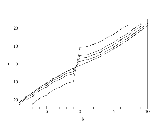
Spectra for one bond defect are shown in Fig. 1 for a subsystem of sites.
The eigenvalues come in pairs () due to the particle-hole
symmetry of the problem.
For a homogeneous system, , one finds the slightly bent curve known
from previous investigations [15, 13].
For a weak defect, one can see a shift of the dispersion curve which is upward
for positive and downward for negative ones. This shift
becomes stronger as the bond becomes weaker. In addition, oscillations appear which
also increase for weaker bonds. Most importantly, however, more and more of the low
follow a steeper dispersion curve as approaches zero. This
curve has a slope approximately twice as large as for the homogeneous system and no wiggles
and represents the result one obtains directly for the system with a free end.
Thus the spectrum with the defect is a mixture of those for the two cases and .
For a strong defect, the situation is basically the same. However, here the two lowest eigenvalues and play a special role because they approach zero as . This moves the left and right part of the spectra two units apart. This feature can be understood from the correlations in this limit. The two
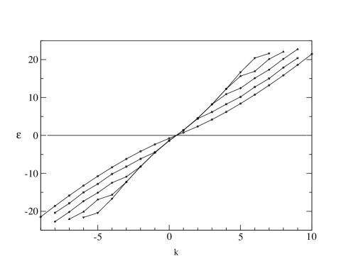
Left : Weak defects, (from bottom to top in the right part of the figure).
Right : Strong defects, (also from bottom to top). The lines are guides for the eye.
The numbering is such that positive have positive values of .
localized states below and above the band then exhaust the local Hilbert space at the two bond sites and effectively cut the system. Thus for and the diagonal term gives one eigenvalue zero. The other one appears because the remaining part of the subsystem has an odd number () of sites. It is absent, if the full subsystem has sites. Then the spectrum for is exactly the same as for sites and up to the remaining zero eigenvalue.
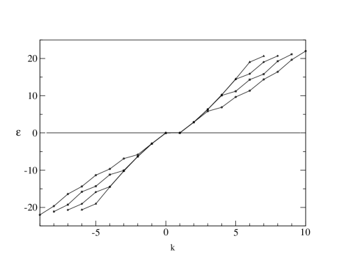
Left : weak bond defects. Right : strong bond defects. The parameters are the same as in Fig. 1.
Spectra for two bond defects are shown in Fig. 2. These were calculated by finding
the eigenfunctions of for a total system of size numerically. This
introduces small finite-size effects but these are not visible on the scale of the figure.
There
is a shift of the curves as for a single defect, but now it affects eigenvalues
if the defects are weak. Thus a gap is opened in the spectrum. For
all diverge. This is reflects the fact that the
subsystem is, in this limit, completely decoupled from the rest and the ground state
becomes a product state. Then has one eigenvalue 1 if all single-particle
levels are unoccupied and all other eigenvalues vanish. If the defects are strong,
two go to zero while the remaining eigenvalues again diverge. The
zero eigenvalues are related to the localized states at the two bonds which belong
to the subsystem as well as to the environment. The ground state then has four
components which differ by the location of the electrons on the two bonds and the four
resulting eigenvalues 1/4 of are produced by the two vanishing .
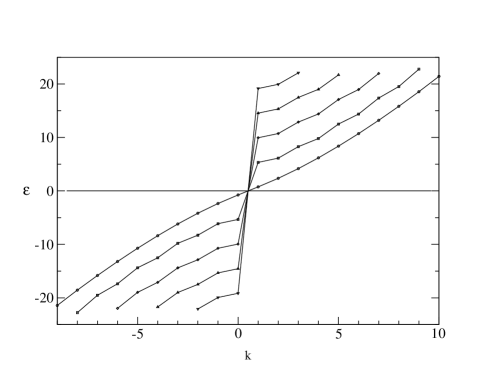
For comparison, the spectra for two site defects are shown in Fig. 2. These defects destroy the particle-hole symmetry of the problem and therefore the spectrum of the is in general no longer symmetric with respect to zero. Apart from that, it shows the same features as for two bond defects. In particular, also the site defects cut off the subsystem if the site energy becomes large and thus all except two diverge for . In this limit, the reflection symmetry of the spectrum is also restored.
III Entanglement entropy
Using the values of the or the , one can obtain the the entanglement entropy from (13),(14). Results for single bond defects are shown in Fig. 4 for system sizes between and .
The plot on the right hand side shows that varies logarithmically with in all cases. There is no indication of a -term as found in [4]. There is only a small variation of the slope with and its asymptotic value can be determined very well by an extrapolation in . It is remarkable that one can see this logarithmic behaviour so well, since for all sizes considered here only about 20 single-particle eigenvalues contribute if the accuracy is set to . Thus one is far away from a limit in which the eigenvalue spectrum becomes dense and where the logarithmic dependence could result from the density of states.
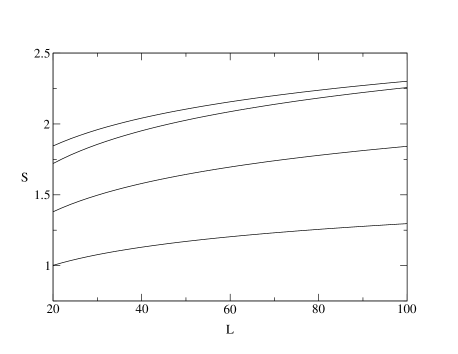
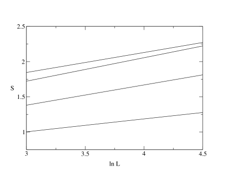
Thus we find that the entanglement entropy has the same form (1)
as for the homogeneous system, but with an effective value which
depends on the strength of the defect. The same holds for two bond defects
and also for site defects (see below). We first discuss the case of one bond
defect further.
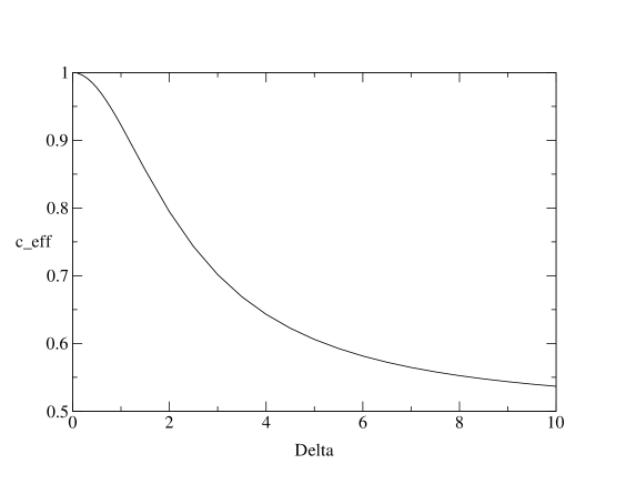
The asymptotic value of , determined by extrapolating the data from , is shown in Fig. 5 as a function of the defect strength.
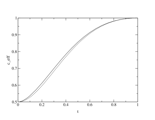
One sees that it varies smoothly between the limits for a subsystem with a free end and for a homogeneous system. The figure shows only for because one finds that is symmetric under .
One can try to find a simple analytic function which fits the numerical curve in Fig. 5. Since the defect is characterized by the scattering phases, one could expect that depends on these. Because one is dealing with an asymptotic property, the phase shifts at the Fermi surface should enter. These are given by
| (15) |
for functions symmetric and antisymmetric about the defect, respectively. One is then lead to the expression
| (16) |
The expression in the brackets also appears (as an exponent) if one calculates the time
autocorrelation function of a spin in an XX spin chain with a bond defect
[16]. The function
(16) has the correct limits for and and is symmetric under
. As can be seen from the figure, it approximates the numerical data
quite well. The deviations are less than , but the agreement is not perfect.
Especially for , the data do not seem to vary quadratically in but
with a power 1.8. Replacing the power 2 in (16) by this value improves the
fit over the whole intervall substantially. The deviations become less than
and are almost invisible on the scale of the figure.
The two terms in (16) can be viewed as the contributions of the unperturbed and the perturbed interface, respectively. One can understand this result from the form of the single-particle spectrum. In the previous section it was found that it consists of two pieces. If one assumes that in the limit the levels in these two branches become equidistant and dense such that (for positive )
| (17) |
where depends on such that for and for and is a constant, the entanglement entropy can be written as
| (18) |
Here is given by the bracket in (14) and the factor of 2 in front takes care of the negative levels. Denoting the second integral by , one obtains
| (19) |
Thus each interface brings its own amplitude for the logarithm : the unperturbed one and the perturbed one . For the homogeneous system the bracket must have the value 1/3, from which follows. Therefore (19) gives for
| (20) |
If the exact dependence of on were known, one could evaluate the
integral and determine in this way. The oscillations of the
which are neglected in (17) could also be included.
The discussion so far has dealt with one defect. However, one can apply it also to the case of two defects. The results of Section III show that then the lowest eigenvalues are just missing and one also finds that the gap in the spectrum for two defects corresponds roughly to the bending point in the spectrum for one defect. Therefore one has only the second region in (17) and finds instead of (19)
| (21) |
from which the value of can be read off. This also gives the relation
| (22) |
between the effective c-values for two defects and for one defect. Due to the
lower accuracy of the calculations for two defects, this relation could not be
checked precisely, but the deviations are less than some percent and vanish near
and .
Results for the case of one site defect are shown in Fig. 6. Here the entanglement entropy is symmetric under and only positive values of have to be considered. One sees that decreases again from the value 1 to 1/2 as the perturbation becomes stronger, because the defect cuts the chain in the limit and thus acts like a bond with or .
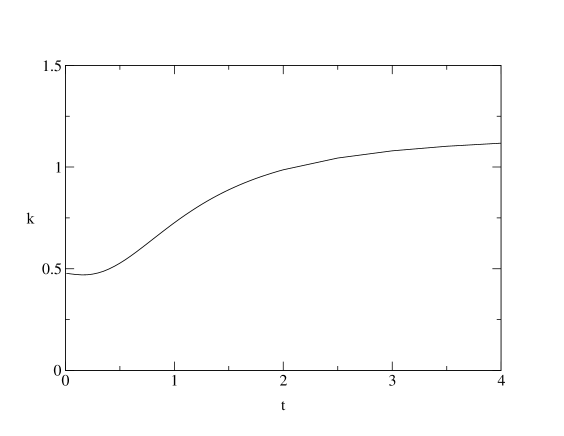
Finally, we present results for the constant in the entropy, see (1). They were obtained by extrapolating from the values . As Fig. 7 shows, this quantity is not symmetric under for one bond defect. Rather it increases from about 0.5 for to about 1.2 for large values of , with a small initial dip (which depends sensitively on ). At we find a value which is in agreement with the findings in [9] but differs slightly from the value obtained from the asymptotic analysis in [10]. The limiting value for is found to differ from the value at by . If one considers systems with an odd number of sites for , this also holds and follows in this case directly from the identity of the single-particle spectra up to one zero eigenvalue (which contributes ) noted in Section III. The relatively large value of can make the entropy with a defect larger than without one if the subsystem is small enough (compare Fig. 4). However, in the limit the effect of the reduced always dominates and leads to a reduction of the entanglement.
IV Conclusion
We have investigated a chain of free electrons in its ground state at half filling.
The entanglement properties were calculated for the case of one or
two defects located at the contact points between the subsystem and the rest of the
chain. The density-matrix spectra were seen to differ in a characteristic way from
those for a homogeneous system. Nevertheless, the logarithmic dependence of
the entanglement entropy on the size persists, only the amplitude changes
and becomes dependent on the defect strength.
The mechanism could be described by a simple model based on the features of
the single-particle spectra. A simple approximate formula for the effective central
charge was also given. Although we focussed on bond defects, the same
features are found for site defects. The logarithmic law means that the system remains
critical, as expected for a localized perturbation. In the two-dimensional system
associated with the quantum chain, the defect becomes a line as noted and used
in [4].
Such a two-dimensional system with a cut (because one considers the reduced density
matrix) and one or two straight defect lines perpendicular to this cut can be mapped
conformally to a strip [14] but the defect lines are bent by
the mapping. For a single defect, the line runs only in the left or right half of the strip,
coming from one point on the boundary and going back to another one.
For two defects, the two lines are attached to different edges and touch in
the center of the strip. The more complicated density-matrix spectra found here must
be related to this feature. It would be interesting to derive them analytically. Also
one wonders if the asymptotic formulae used in [10, 17] to
calculate can be generalized to the present case.
The author thanks K.D. Schotte for discussions and help with the figures.
REFERENCES
- [1] L. Bombelli, R. K. Koul, J. Lee and R. D. Sorkin, Phys. Rev. D 34, 373 (1986)
- [2] M. Srednicki Phys. Rev. Lett. 71, 666 (1993)
- [3] M. B. Plenio, J. Eisert, J. Dreissig and M. Cramer, preprint quant-phys/0405142
- [4] G. C. Levine, Phys. Rev. Lett. 93 266402 (2004)
- [5] C. L. Kane and M. P. Fisher, Phys. Rev. B 46, 15233 (1992)
- [6] Ch. Holzhey, F. Larsen and F. Wilczek, Nucl. Phys. B 424, 443 (1994)
- [7] P. Calabrese and J. Cardy, J. of Statistical Mechanics, P06002 (2004)
- [8] G. Vidal, J. I. Latorre, E. Rico and A. Kitaev, Phys. Rev. Lett. 90, 227902 (2003)
- [9] J. I. Latorre, E. Rico and G. Vidal, Quant. Inf. and Comp. 4, 48 (2004), preprint: quant-ph/0304098
- [10] B.-Q. Jin and V. E. Korepin, J. Stat. Phys. 116, 79 (2004),
- [11] I. Peschel, J. Phys. A 36, L205 (2003)
- [12] S.-A. Cheong and C. L. Henley, Phys. Rev. B 69, 075111 (2004), preprint: cond-mat/0206196
- [13] S.-A. Cheong and C. L. Henley, Phys. Rev. B 69, 075112 (2004)
- [14] I. Peschel, J. of Statistical Mechanics P06004 (2004)
- [15] M.-C. Chung and I. Peschel, Phys. Rev. B 64, 064412 (2001)
- [16] I. Peschel and K. D. Schotte, Z. Physik B 54 305 (1984)
- [17] J. P. Keating and F. Mezzadri, Preprint quant-ph/0407047