Bistable Clustering in Driven Granular Mixtures

Abstract

The behavior of a bidisperse inelastic gas vertically shaken in a compartmentalized container is investigated using two different approaches: the first is a mean-field dynamical model, which treats the number of particles in the two compartments and the associated kinetic temperatures in a self-consistent fashion; the second is an event-driven numerical simulation. Both approaches reveal a non-stationary regime, which has no counterpart in the case of monodisperse granular gases. Specifically, when the mass difference between the two species exceeds a certain threshold the populations display a bistable behavior, with particles of each species switching back and forth between compartments. The reason for such an unexpected behavior is attributed to the interplay of kinetic energy non-equipartition due to inelasticity with the energy redistribution induced by collisions. The mean-field model and numerical simulation are found to agree qualitatively.

I Introduction

Granular fluids are currently attracting growing interest in view of their unusual properties, some of which are not fully understood yet. Moreover, new experiments continue to reveal unexpected phenomena, which have no counterpart in molecular fluids. Clustering, shear instability, non-Maxwellian velocity distributions, long range velocity correlations, non-equipartition in a binary mixture are just a few of these peculiarities gases ; general ; Kadanoff . Recently, another fascinating phenomenon was reported. It is the so called “Maxwell sand daemon” experiment experiment , where a system consisting of inelastic particles enclosed in a two-compartment container is shaken vertically. Particles can flow from one compartment to the other through a small orifice located at a certain height from the basal vibrating plate. For strong shaking, the right and left populations are statistically equal, whereas for weak shaking the system spontaneously breaks the left-right symmetry. The mechanism behind such an unusual ordering process is the clustering induced by inelasticity.

In fact, an imbalance in populations induced by a fluctuation can be amplified, since it causes a larger energy dissipation on the overpopulated side, thus suppressing the outflow from that compartment. At the same time, inflow from the underpopulated compartment is enhanced because of its lower occupation, which results in higher kinetic energies per particle Eggers .

Quite recently, the Twente collaboration Mikkelsen investigated the behavior of a bidisperse granular mixture of small and large particles using a similar experimental setup. Their experiments demonstrated that a bidisperse compartmentalized granular mixture has a tendency to cluster competitively. Depending on the shaking strength, one can observe different asymptotic configurations.

Theoretical treatments of granular gases in compartmentalized systems range from phenomenological flux models Eggers ; Mikkelsen ; Lohse ; Lohse1 ; Lohse2 ; Droz ; Droz1 ; Droz2 , to molecular dynamics dererumpallettarum ; ceccojcp , to more refined kinetic approaches Brey . Whereas the full solution of the inelastic Boltzmann equation remains a formidable task, a simple set of mean-field dynamical equations can be derived Puglio ; Conti . According to this method, the kinetic temperatures and the occupation numbers in each compartment are assumed to be the only relevant dynamical variables and treated on equal footing, a technique which naturally lends itself to capture the more complex phenomenology expected in mixtures.

Here we study a binary mixture of inelastic hard disks in a two-compartment system. The two species have different masses, are subjected to gravity and driven by a vibrating base. We extend the mean-field treatment of ref.Puglio and compare its predictions with the results of even-driven simulations.

The paper is organized as follows: after introducing our model in section II, we develop our mean-field treatment in section III. In section IV we report the predictions of our model and summarize our findings with a mean-field “phase diagram”, where the boundaries between different regimes are studied as function of the control parameters. In section V we turn to the event-driven simulation and find qualitative agreement with the previous picture. Finally, in section VI, we present our conclusions.

II The model

Let us consider a two-dimensional rectangular container with horizontal and vertical sides of length $L_{x}$ and $L_{z}$, respectively, divided in two equal compartments by a wall of height $h<L_{z}$. The box contains a mixture of $\mathcal{N}_{1}$ and $\mathcal{N}_{2}$ inelastic hard disks of diameter $\sigma$ and masses $m_{1}$ and $m_{2}$, respectively. The disks are subjected to a gravitational force acting along the negative $z$ direction and are fluidized by the sawtooth-like movement of the base, which oscillates with frequency $\nu$ and amplitude $A$. The side and top walls are fixed, and particles collide with them in a perfectly elastic fashion. The collisions between particles are inelastic, and will be described by means of a velocity-dependent coefficient of restitution Daniela : $\alpha(V_{n})$,

$$\alpha(V_{n})=\left\{\begin{array}[]{lll}1-(1-r)\left(\frac{|V_{n}|}{v_{0}}\right)^{\frac{3}{4}}&\mbox{ for }&|V_{n}|<v_{0}\\ r&\mbox{ for }&|V_{n}|>v_{0}\,\,,\end{array}\right.$$

where $V_{n}$ is the pre-collisional relative velocity along the direction joining the centers of the two particles, $v_{0}=\sqrt{g\sigma}$ is a cutoff velocity and $g$ is the gravitational acceleration. For large values of relative normal velocities, the function $\alpha(V_{n})$ assumes a constant value $r$, while for $V_{n}\to 0$ the elastic behavior $\alpha(0)=1$ is approached according to a power law. We checked the robustness of our results with respect to variations in $v_{0}$. For the sake of simplicity, the law $\alpha(V_{n})$ is the same for all types of collision. Binary collision between a particle of species $\mu$ and another particle of species $\nu$ change pre-collisional velocities $\bf{v}_{1}$ and $\bf{v}_{2}$ into post-collisional velocities $\bf{v}_{1}^{\prime}$ and $\bf{v}_{2}^{\prime}$ according to:

$${\bf v}_{1}^{\prime}={\bf v}_{1}-\mu_{\nu\mu}(1+\alpha)(\widehat{\bf{n}}\cdot{\bf v}_{12})\widehat{{\bf n}}$$ (1)

$${\bf v}_{2}^{\prime}={\bf v}_{2}+\mu_{\mu\nu}(1+\alpha)(\widehat{\bf{n}}\cdot{\bf v}_{12})\widehat{{\bf n}}$$ (2)

where $\mu_{\mu\nu}=m_{\mu}/(m_{\mu}+m_{\nu})$, $\widehat{\bf{n}}$ is a unit vector directed from the center of the particle of type $\mu$ to the center of particle $\nu$, and $\bf{v}_{12}=\bf{v}_{1}-\bf{v}_{2}$. Inter-particle collisions conserve momentum, but result in an energy loss proportional to $(1-\alpha^{2})$.

The space of the control parameters is large since the system properties are functions of several dimensionless quantities, such as the coefficient of restitution $r$, the total number of particles $\mathcal{N}=\mathcal{N}_{1}+\mathcal{N}_{2}$, the mass ratio, the ratio of lengths $L_{x}/\sigma$, the ratio between the typical energy transferred from the piston to the particles and their gravitational energy, and so on. We study the system behavior by considering a combination of the above parameters,

$$R=\frac{gh}{A^{2}\nu^{2}}(1-r^{2})\frac{\mathcal{N}^{2}\sigma^{2}}{L_{x}^{2}}\,,$$ (3)

whose relevance has been pointed out in Lohse1 . The dimensionless parameter $R$ decreases as the driving intensity $A\nu$ increases, while increases as the dissipation becomes larger.

III Mean-Field Theory

In this section we shall extend the mean-field treatment of the compartmentalized inelastic gas, which was introduced in refs. Puglio ; Conti , to include the case of different species, non-equal occupation numbers and different partial temperatures of the system. In a realistic scenario, the presence of strong inhomogeneity and of the ensuing gradients make the analysis of the Boltzmann transport equation far too complex. The Twente collaboration proposed a simple flux model Lohse , while in ref. Puglio a simple coarse-grained version of the Boltzmann equation was introduced, leading to equations for the occupation numbers that appear to be very similar to those of the flux model. Such an approach has also the advantage of treating occupation numbers and granular temperatures on equal footing. In the following, we extend this method to the case of a granular mixture.

In order to obtain our mean-field equations we shall make a series of simplifying assumptions:

1. the system properties are regarded as homogeneous within each compartment, so that only the numbers of particles and the kinetic energy of the two species in each compartment are the only relevant variables;

2. the coefficient of restitution is velocity-independent, i.e. $\alpha(V_{n})=r$;

3. the driving mechanism is spatially homogeneous and representable by means of a stochastic thermostat;

4. the velocity distributions are Gaussian, and their variances are derived in a self-consistent fashion;

5. the effect of collisions is adequately described by the inelastic homogeneous Boltzmann equation;

6. particles whose kinetic energy exceeds an assigned threshold switch to the adjacent compartment at a fixed rate $\tau_{s}^{-1}$.

The assumption of spatial homogeneity allows us to write the phase-space distribution function for species $\mu$ (with $\mu=1,2$) as

$$f_{\mu}({\bf r},{\bf v},t)=f_{a,\mu}({\bf v},t)\,\,.$$

Here $a=1$ when point ${\bf r}$ falls within the left side of the container (relative to the barrier) and $a=2$ when ${\bf r}$ falls on the right side. Such a coarse-graining procedure allows us to write the following Boltzmann-like equation:

$$\partial_{t}f_{a,\mu}({\bf v},t)=\sum_{\nu=1}^{2}I_{\mu\nu}[{\bf v}|f_{a,\mu},f_{a,\nu}]+{\cal B}f_{a,\mu}+{\cal X}[{\bf v}|f_{a,\mu},f_{b,\mu}]\,\,,$$ (4)

where $I_{\mu\nu}$ is the collision term which describes the effect of inelastic collisions among particles belonging to the same compartment, ${\cal B}f_{a,\mu}$ represents the action of the stochastic driving force associated to the heat bath, and ${\cal X}[{\bf v}|f_{a,\mu},f_{b,\mu}]$ represents the flow of particles of species $\mu$ between the two compartments.

The integral $I_{\mu\nu}$ describing collisions between a particle of type $\mu$ and a particle of type $\nu$ can be represented as

$$I_{\mu\nu}[{\bf v}_{1}|f_{a,\mu},f_{a,\nu}]=\sigma\int d{\bf v}_{2}\int^{\prime}d\widehat{{\bf n}}(\widehat{{\bf n}}\cdot{\bf v}_{12})\left(\frac{1}{r^{2}}f_{a,\mu}({\bf v}_{1}^{\prime\prime})f_{a,\nu}({\bf v}_{2}^{\prime\prime})-f_{a,\mu}({\bf v}_{1})f_{a,\nu}({\bf v}_{2})\right)\,,$$ (5)

where doubly primed symbols stand for pre-collisional velocities and the $r^{2}$ factor in the denominator stems from inelasticity vannoije .

The number of particles of species $\mu$ in compartment $a$ is defined as

$$n_{a,\mu}(t)=\int d{\bf r}\int d{\bf v}f_{a,\mu}({\bf v},t)\ .$$ (6)

Similarly, we define four partial granular temperatures:

$$n_{a,\mu}T_{a,\mu}(t)=\int d{\bf r}\int d{\bf v}\frac{m_{\mu}v^{2}}{2}f_{a,\mu}({\bf v},t)\ .$$ (7)

Now we derive the governing equations for occupation numbers and kinetic temperatures. By integrating eq. (4) with respect to velocity ${\bf v_{1}}$, and recalling that both the collision integral and the heat bath term conserve the number of particles in each compartment, one can see that the rate of change of $n_{a,\mu}$ is determined solely by the exchange term ${\cal X}$:

$$\partial_{t}n_{a,\mu}(t)=\int d{\bf v}{\cal X}[{\bf v}|f_{a,\mu},f_{b,\mu}]\,\,.$$ (8)

According to the assumption of point 6 (see list above), the exchange term has the form

$${\cal X}[{\bf v}|f_{a,\mu},f_{b,\mu}]=-\frac{1}{\tau_{s}}\theta(|{\bf v}|-u_{s})[f_{a,\mu}({\bf v},t)-f_{b,\mu}({\bf v},t)]\,\,.$$ (9)

In other words, one assumes that particles having velocities larger than a given threshold $u_{s}$ cross the barrier with probability $\tau_{s}^{-1}$ per unit time. The resulting equation for $n_{a,\mu}$ is

$$\frac{{\rm d}n_{a,\mu}(t)}{{\rm d}t}=-\frac{V}{\tau_{s}}\int{\rm d}{\bf v}[f_{a,\mu}({\bf v},t)-f_{b,\mu}({\bf v},t)]\theta(|{\bf v}|-u_{s})\,.$$ (10)

Mathematical convenience suggests an additional assumption for the form of the heat bath operator ${\cal B}$: we replace the effect of the periodic vibration of the piston with a sequence of uncorrelated random kicks whose amplitude is distributed according to a Gaussian Puglisi2 ; Vibrated . The effect of this stochastic acceleration is described by the Langevin equation

$$\frac{{\rm d}{\bf v}_{i}}{{\rm d}t}=\hat{\bf{\xi}_{i}}\,,$$ (11)

where ${\bf{\xi}_{i}}$ is a a Gaussian white noise with zero average, and variance given by

$$\langle{\xi}_{i}(t){\xi}_{j}(t^{\prime})\rangle=\eta^{2}\delta_{ij}\delta(t-t^{\prime})\,.$$ (12)

Here $\eta^{2}$ measures the intensity of the stochastic driving. This leads to the following forcing term:

$${\cal B}f_{a,\mu}=\frac{\eta^{2}}{2}\frac{\partial^{2}}{\partial v^{2}}f_{a,\mu}({\bf v},t)\,.$$ (13)

Notice that particles receive an energy proportional to their masses. Next, we consider the time evolution of partial kinetic energies $T_{\mu}$, which is obtained by multiplying eq.(4) by $m_{\mu}{\bf v}^{2}/{2}$ and integrating over velocity.

$$\frac{1}{V}\partial_{t}(n_{a,\mu}T_{a,\mu})=\frac{m_{\mu}}{2}\sum_{\nu}\int d{\bf v}v^{2}I_{\mu\nu}[{\bf v}|f_{a,\mu},f_{a,\nu}]+\frac{m_{\mu}}{2}\int d{\bf v}v^{2}{\cal B}f_{a,\mu}$$

$$-\frac{m_{\mu}}{2\tau_{s}}\int{\rm d}{\bf v}v^{2}[f_{a,\mu}({\bf v},t)-f_{b,\mu}({\bf v},t)]\theta(|{\bf v}|-u_{s}),\qquad$$ (14)

Finally, in order to derive an explicit expression for the governing equations we assume Gaussian velocity distributions:

$$f_{a,\mu}({\bf v},t)=\frac{n_{a,\mu}}{V}\frac{m_{\mu}}{2\pi T_{a,\mu}}\exp\left(-\frac{m_{\mu}{\bf v}^{2}}{2T_{a,\mu}}\right)\,.$$ (15)

Inserting eq. (15) into equation (10) we obtain

$$\frac{{\rm d}n_{a,\mu}(t)}{{\rm d}t}=\frac{1}{\tau_{s}}\left[n_{b,\mu}e^{-T_{\mu s}/T_{b,\mu}}-n_{a,\mu}e^{-T_{\mu s}/T_{a,\mu}}\right]\,,$$ (16)

where the temperature $T_{\mu s}$ is given by $T_{\mu s}=\frac{1}{2}m_{\mu}u_{s}^{2}$ and the right-hand side represents the difference between the incoming flux and the outgoing flux of compartment $a$, as in the flux model.

The calculations involving the collision term are quite lengthy, but straightforward. Here we will not report the detailed derivation, which can be found in refs. Garzo ; Equipart . The final form of the governing equation for the granular temperature (say, of species 1 in compartment a) is:

$$n_{a,1}(t)\frac{{\rm d}T_{a,1}(t)}{{\rm d}t} = -\frac{2}{\tau_{s}}\left[n_{a,1}T_{a,1}e^{-T_{1s}/T_{a,1}}-n_{b,1}T_{b,1}e^{-T_{1s}/T_{b,1}}\right]$$ (17)

$$- \frac{1}{\tau_{s}}\left[(n_{a,1}e^{-T_{1s}/T_{a,1}}-n_{b,1}e^{-T_{1s}/T_{b,1}})(2T_{1s}-T_{a,1})\right]$$

$$- \gamma_{11}n_{a,1}T_{a,1}-\gamma_{12}m_{1}n_{a,1}\left(\frac{T_{a,1}}{m_{1}}+\frac{T_{a,2}}{m_{2}}\right)$$

$$- \kappa_{12}m_{1}n_{a,1}(\frac{T_{a,1}-T_{a,2}}{m_{1}+m_{2}})+m_{1}\eta^{2}n_{a,1}\,\,,$$

The corresponding equations for other choices of species and compartment are obtained by simple substitution of indices. where the coefficients $\gamma_{\mu\nu}$ and $\kappa_{\mu\nu}$ are given by

$$\gamma_{\mu\nu}=(1-r^{2})\sigma\mu_{\nu\mu}^{2}\frac{n_{a,\nu}}{A}\left(\frac{2T_{a,\mu}}{m_{\mu}}+\frac{2T_{a,\nu}}{m_{\nu}}\right)^{1/2}\,,$$ (18)

$$\kappa_{\mu\nu}=2(1+r)\sigma\mu_{\nu\mu}^{2}\frac{n_{a,\nu}}{A}\left(\frac{2T_{a,\mu}}{m_{\mu}}+\frac{2T_{a,\nu}}{m_{\nu}}\right)^{1/2}\,.$$ (19)

The constant $A$ is the area available to the particles in each compartment. $\gamma_{\mu\nu}$ takes into account the effect of collisions between particles belonging to species $\mu$ and $\nu$, respectively. Interestingly, $\kappa_{\mu\nu}$ does not vanish in the elastic limit ($r\to 1$), since it is associated with the restoring mechanism which tends to equalize the partial kinetic temperatures of two different components in a standard fluid.

The complete set of equations (16) and (17) consists of eight non-linear coupled equations, of which only six are independent, because the occupation numbers – being globally conserved – have to satisfy $n_{1,\mu}+n_{2,\mu}=\mathcal{N}_{\mu}$.

IV The mean-field scenario

To be able to compare the predictions of the proposed mean-field model against the results of numerical simulation, we need to introduce a suitable definition of $R$ (eq. 3) for the case of our thermal bath. Specifically, we rewrite the first factor of equation (3) as $mgh/(P^{2}/m)$, where $P$ is the typical momentum transferred to a particle that collides with the piston. We replace the energy scale $mgh$ – associated to barrier crossing – with the analogous scale $T_{\mu s}$, and the transferred momentum scale $P$ with its equivalent for the stochastic forcing of eq. 12, $m\eta\sqrt{\tau_{s}}$. Thus, for the mean-field model, the analogous of eq. 3 can be written as:

$$R_{MF}=\frac{T_{\mu s}}{m_{\mu}\eta^{2}\tau_{s}}(1-r^{2})\frac{N^{2}\sigma^{2}}{L_{x}^{2}}\,.$$ (20)

Obviously we expect the correspondence between $R$ and $R_{MF}$ to be useful only for qualitative comparison of the mean-field model against numerical simulation.

We shall now consider some of the properties of the asymptotic solutions of eqs.(16) and (17). The specific numerical values of the control parameters correspond approximately to those used in the experiments by Mikkelsen .

A symmetric solution, characterized by equal state variables in the two compartments, $n_{1,\mu}=n_{2,\mu}$ and $T_{1,\mu}=T_{2,\mu}$, always represents a fixed point for the governing equations. However, as the parameter $R_{MF}$ increases, such a symmetric fixed point becomes unstable. At small driving intensity or high dissipation the solution ceases to be symmetric and the particles of both species tend to cluster in one of the two compartments. Such a symmetry breaking behavior was studied experimentally and explained in terms of flux models Lambiotte ; Mikkelsen . By numerically integrating eqs.(16) and (17), we are also able to observe the same simmetry-breaking behavior for the case of our mean-field description.

In fig. 1 we show the temporal evolution of occupation numbers for the two species (in a single compartment) for different choices of the driving intensity. We observe two dynamical scenarios. In the first scenario, the occupation numbers approach a stationary symmetry-broken solution via a simple bifurcation (i.e a critical point). This corresponds to the situation considered in ref. Ioepuglio , and occurs for small mass differences or small concentrations ($m_{2}/m_{1}=2$, for example). In the second scenario, the temporal evolution of the occupation numbers approaches a limit cycle so that that particles of each species oscillate back and forth between compartments. This occurs when the difference in mass is large, or when masses are equal but sizes are different enough, in analogy to the observations of Lambiotte et al. Lambiotte .

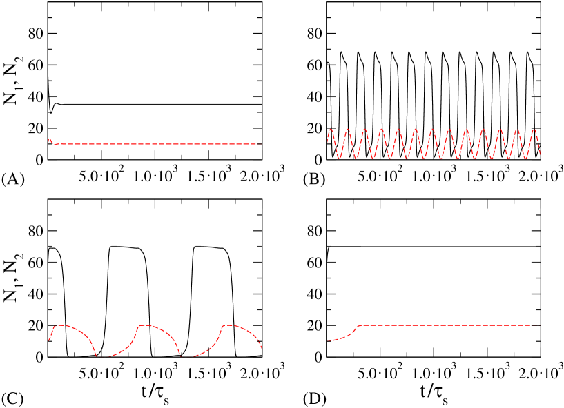
Figure 1: Four different behaviors obtained by varying the dimensionless parameter $R_{MF}$, and keeping the mass ratio $m_{2}/m_{1}=8$ and the population ratio $\mathcal{N}_{1}/\mathcal{N}_{2}=70/20$. The continuous line ($N_{1}$) refers to the light species and the dotted line ($N_{2}$) to the heavy species, both in the right compartment. In panel A ($R_{MF}=6.0$) the asymptotic solution is symmetric. In panel B ($R_{MF}=12$) the occupation numbers oscillate in time. Panel C ($R_{MF}=24$) shows a case where the solution displays oscillations with longer periods. Finally, panel D ($R_{MF}=48$) illustrates a typical simmetry breaking solution, where occupation numbers in the two compartments are different, for each species. The time is measured in units $\tau_{s}$.

Although the system is far from equilibrium and has a finite extension we shall employ the term “phase diagram” in order to stress the existence of different dynamic regimes. The resulting phase diagram in the plane $R_{MF}$ vs. $m_{2}/m_{1}$ is shown in fig. 2. No oscillations can be observed for small mass asymmetry ($\frac{m1}{m2}\simeq 1$) and the crossover from the symmetric phase to the asymmetric phase is similar to what occurs in the case of a one-component system. However, when the mass asymmetry increases ($m_{2}/m_{1}\gtrsim 3$) an intermediate oscillatory regime appears, and no stationary solution is attained anymore.

The effect of concentration on the appearance of oscillations is instead shown in fig. 3. For small concentrations of the heavy species $\mathcal{N}_{2}/(\mathcal{N}_{1}+\mathcal{N}_{2})$ there is a direct crossover, as $R$ decreases, from the asymmetric “phase” to the symmetric “phase”. When the concentration $\mathcal{N}_{2}/(\mathcal{N}_{1}+\mathcal{N}_{2})$ of the heavy particles increases, there appears an island of the oscillating “phase”, which subsequently disappears when the concentration of heavy particles becomes too large. The oscillation period decreases as $R_{MF}$ decreases and is larger near the boundary between the “broken phase” and the “oscillatory phase”. In the following, in order to simplify the notation, we shall denote $N_{1}=n_{1,1}$ and $N_{2}=n_{2,1}$.

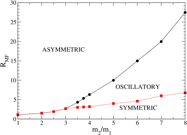
Figure 2: Phase diagram for a system with $\mathcal{N}_{1}=70$ light particles and $\mathcal{N}_{2}=20$ heavy particles. The transition values of $R_{MF}$ are plotted as functions of the mass ratio $m_{2}/m_{1}$.

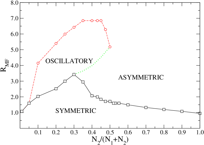
Figure 3: Phase diagram for a system with $\mathcal{N}_{1}+\mathcal{N}_{2}=90$ particles as function of $\mathcal{N}_{2}/(\mathcal{N}_{1}+\mathcal{N}_{2})$, for a mass ratio $m_{2}/m_{1}=4$.

V Numerical experiments

In order to verify whether the hard disk model correctly describes experimental observations Lohse and also to probe the qualitative validity of our mean-field scenario, we now turn to discuss a set of numerical experiments. We confirm that the behavior of the mixture, as already revealed by mean-field calculations, strongly depends on the specific choice of control parameters.

The simulated dynamics consists of a succession of ballistic trajectories and inter-particle or wall-particle collisions. With respect to the code employed previously (see references Daniela and convection ) we introduce a dividing, elastic barrier, visibile in fig. 4. The two species are chosen to be smooth rigid disks of equal diameters $\sigma=0.5$ cm and unequal masses $m_{1}=6.545\cdot 10^{-2}g$ and $m_{2}=5.236\cdot 10^{-1}g$, respectively. The mixture is composed of $\mathcal{N}_{1}=60$ light particles and $\mathcal{N}_{2}=30$ heavy particles. The vibrating base is driven according to a symmetric sawtooth waveform and the vibration amplitude is set to $A=0.4\sigma$. Finally, the width $L_{x}$ of the compartment ranges from $34\sigma$ to $240\sigma$, while its vertical dimension is $L_{z}=82.4\sigma$, and the height of the dividing wall is $h=12\sigma$.

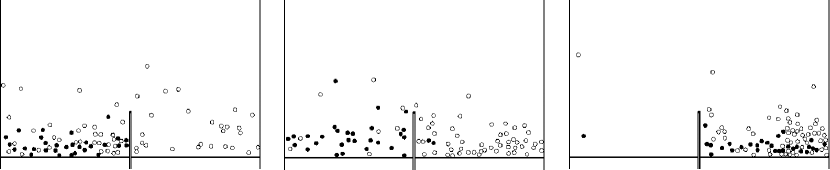
Figure 4: Typical snapshots of the process described in Section V. Open circles indicate the light particles, black circles the heavy particles. System parameters are $\nu=47$ Hz, $L_{x}=34\sigma$, $m_{2}/m_{1}=8$, $\mathcal{N}_{1}=60$, $\mathcal{N}_{2}=30$, $A=0.4\sigma$ and $\sigma=0.5cm$.

Our observables are computed as instantaneous averages in the case of global quantities, such as the occupation numbers for the two species and the partial kinetic energy per particle, and as time averages (ergodic averages) for other quantities, such as densities, temperatures and velocity distribution functions.

For strong driving (i.e. small $R$, as already shown in the mean-field case) the system approaches a stationary state where the number of particles in each compartment, or average, is the same. Such a steady state is maintained by a continuous exchange of particles of both species between the compartments. The average kinetic energies are sufficiently high so that particles can jump over the barrier. Upon increasing $R$ the symmetry is spontaneously broken: the system can either attain an asymmetric stationary state, or approach a limit cycle where populations keep switching back and forth between compartments in a coherent fashion. These scenarios are shown in figures 5 for $m_{2}/m_{1}=8$, $r=0.85$ and $\nu=47$ Hz, where the crossover from one regime to the other occurs by varying the value of $L_{x}$. For $L_{x}=160\sigma$ and $L_{x}=120\sigma$ the particles are nearly equidistributed among the compartments. On the other hand, when the system is narrow enough ($L_{x}=62\sigma$) the particles – after an initial transient – tend to localize in the same compartment for time intervals longer than our observation time. However, when we change the width of the compartment from $L_{x}=62\sigma$ to $L_{x}=80\sigma$, pronounced oscillations appear and the populations appear to move back and forth. The global picture is consistent with our previous mean-field analysis.

We also explore the effect of varying the driving frequency at fixed $L_{x}$, and we find that the breakdown of the symmetric stationary state still occurs, as shown in fig. 6. Moreover, the oscillatory behavior only appears for large mass asymmetry. On the other hand, the time series of fig. 7 shows that the corresponding mass asymmetry ($m_{2}/m_{1}=2$) is not large enough to induce clean oscillations, so that only the phenomenology of one-component driven granular gases can be observed.

Finally, we remark that the same kind of oscillations may occur when the diameters of the two species are different enough, even in the case of equal masses (data not shown).

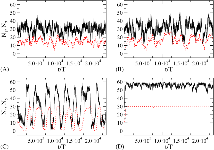
Figure 5: Number of light particles (solid line, $N_{1}$) and heavy particles (dotted line, $N_{2}$) in the left compartment, as a function of time, for different values of $L_{x}$: $L_{x}=160\sigma$ (A), $L_{x}=120\sigma$ (B), $L_{x}=80\sigma$ (C) and $L_{x}=62\sigma$ (D). System parameters: $r=0.85$, $\nu=47$ Hz (period $T=1/\nu$), $A=0.4\sigma$, $\sigma=0.5cm$ and $m_{2}/m_{1}=8$. The panels correspond to $R=5.8$ (A), $10.4$ (B), $23.4$ (C), $39.0$ (D).

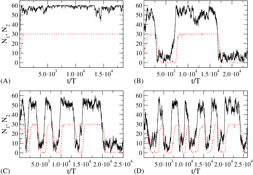
Figure 6: Number of light particles (solid line, $N_{1}$) and heavy particles (dotted line, $N_{2}$) in the left compartment, as a function of time, for different driving frequencies $\nu$ (period $T=1/\nu$): $\nu=37$ Hz (A), $\nu=47$ Hz (B), $\nu=50$ Hz (C), $\nu=52$ Hz (D). System parameters: $r=0.85$, $L_{x}=68\sigma$, $A=0.4\sigma$, $\sigma=0.5~{}cm$ and $m_{1}/m_{2}=8$.

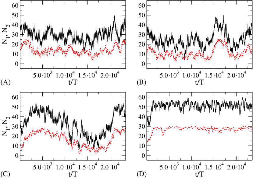
Figure 7: Number of light particles (solid line, $N_{1}$) and heavy particles (dotted line, $N_{2}$) particle in the left compartment, as a function of time, for different choices of $L_{x}$: $L_{x}=240\sigma$ (A), $L_{x}=220\sigma$ (B), $L_{x}=200\sigma$ (C) and $L_{x}=160\sigma$ (D). System parameters: $\nu=47$ Hz, $A=0.4\sigma$, $\sigma=0.5cm$ and $m_{2}/m_{1}=2$. The panels correspond to $R=2.6$ (A), $3.1$ (B), $3.7$ (C), $5.8$ (D).

Let us consider in more detail the oscillatory behavior we observe (for example, refer to panel C of figure 6). After an initial clustering of both species in a compartment – say the left – a net rightward flux of light particles establishes and persists until a sufficient number of them have changed compartment. At this point the heavy particles, too, start jumping to the right, eventually creating in the right compartment a cluster of both species which is totally similar to the initial situation of the left compartment. After reaching this stage, the process repeats itself in the opposite direction.

Such a peculiar behavior has its origin in the mass and/or size difference between the two species and in the associated breakdown of energy equipartition that occurs in a binary vibrated granular gas Feitosa ; Pagnani ; Ciroart . Krouskop and Talbot Talbot studied how the mass ratio affects the exchange of energy of each species and computed the average energy change of a particle of species $\mu$ colliding with a particle of species $\nu$. Assuming that each component has a Maxwell velocity distribution and a partial temperature $T_{\mu}$, the average energy change in 2D is

$$\Delta E_{\mu\nu}=\mu_{\mu\nu}\frac{(1+r)}{2\sqrt{2}}\biggl{[}(1+r)\frac{T_{\nu}m_{\mu}+T_{\mu}m_{\nu}}{m_{\mu}(m_{\mu}+m_{\nu})}-2\frac{T_{\mu}}{m_{\mu}}\biggr{]}\,.$$ (21)

Such an equation shows that for $T_{2}/T_{1}>1$ a light particle – on average – gains energy on colliding with a heavy particle. In our case, the imbalance in temperatures is guaranteed by the fact that heavy particles receive more energy than light ones when colliding with the vibrating base. Such an imbalance is roughly proportional to the mass ratio. Thus heavy particles are able to gain more energy from the driving base, and they can also tranfer it to light particles, effectively heating them. Since the system is not in equilibrium, kinetic temperatures depend on the particle numbers in each compartment and are not known a priori.

In order to check the validity of the above argument, we focused on the steady-state dynamics between transitions, and numerically evaluated the partial temperatures $T_{1}$ and $T_{2}$ in the compartment hosting the majority of heavy particles. Such temperatures mainly depend on the number $\tilde{N}$ of light particles, while they are not signifcantly affected by the number of heavy particles, because the latter population is basically constant between transitions (see fig. 8). On inserting the above partial temperatures into equation (21), and weighting the energy changes with the numerically evaluated collision frequencies, we obtain the average energy changes per particle and per collision, separately for each species:

$$\Delta K_{1}=\frac{\Delta E_{11}M_{11}+\Delta E_{12}M_{12}}{M_{11}+M_{12}}$$ (22)

and

$$\Delta K_{2}=\frac{\Delta E_{21}M_{12}+\Delta E_{22}M_{22}}{M_{22}+M_{12}}\,\,.$$ (23)

Here $M_{\mu\nu}$ represents the number of collisions per unit time between species $\mu$ and $\nu$. Fig. 9 shows $\Delta K_{1}$ and $\Delta K_{2}$ as a function of ${\tilde{N}}$. We observe that light particles, on average, gain energy. Such a gain increases as ${\tilde{N}}$ decreases, because in this situation $M_{12}$ is much larger than $M_{11}$. Thus light particles are more likely to jump into the empty compartment, leaving the heavy ones behind. At this point the heavy particles – no longer transferring energy to the other species – become more energetic and also move to the other compartment, joining the light particles once more.

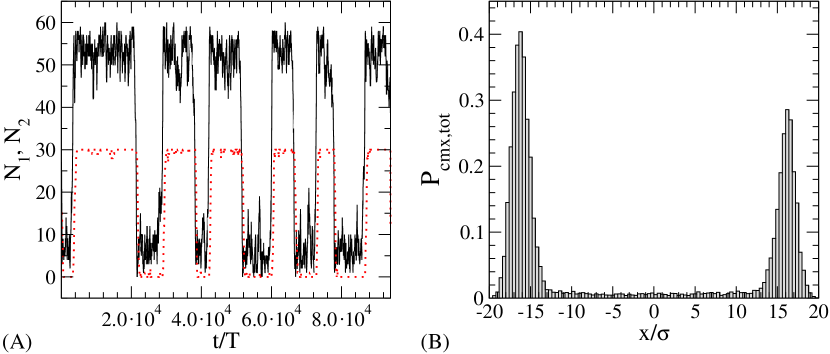
Figure 8: Panel A: time evolution of the occupation numbers $N_{1}$ and $N_{2}$ in the left compartment. Panel B: probability distribution of the horizontal position $x$ of the center of mass (whole system). The left-right asymmetry is due to the limited size of the sample used to compute the histogram. System parameters are $\nu=47$ Hz, $A=0.8\sigma$, $L_{x}=68\sigma$ and $m_{2}/m_{1}=8$.

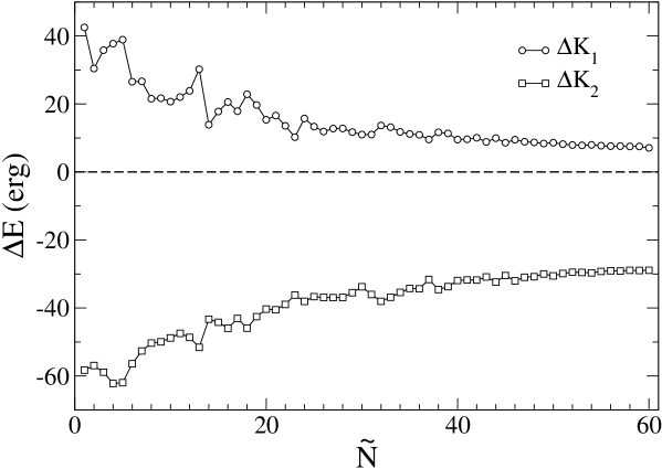
Figure 9: Average energy change for particle-particle collisions, as a function of the number of light particles $\tilde{N}$ present in the compartment where the majority of the heavy particles is located. $\Delta K_{1}$ (open circles) and $\Delta K_{2}$ (squares) correspond to the energy change for light and heavy particles respectively, in the full compartment.

Let us now consider in more detail the statistical properties of the system by analyzing a particular case shown in fig. 8A. One can observe that the occupation numbers fluctuate around well defined plateau values for periods as long as several thousands driving cycles (of duration $T\equiv 1/\nu$).

Interestingly, the distribution of the horizontal position of the center of mass displays a double peak structure, indicating that the system spends most of the time in configurations where the majority of the particles is on one side – an asymmetric situation.

We can better study the switching dynamics of fig.8A by defining a collective residence time $\tau$ as the period during which at least $80$% of the heavy particles persist in a given compartment. The ensuing distribution of residence times is shown in fig. 10. The average residence time is about $6\cdot 10^{3}T$ and the distribution appears to be exponential. In order to ascertain whether the oscillations are periodic, as reported by Lambiotte et al. Lambiotte and predicted by our mean-field model, we study the signal of fig. 8 in the frequency domain. The resulting power spectrum $P(\omega)$ is shown in the inset of fig. 10 and displays no evidence of periodicity. As a further check, we generated a “synthetic” bistable signal by assuming that the occupation numbers of the heavy species in each compartment can assume only two values (say $N_{2}$ and $0$), and that the residence times are randomly distributed according to an exponential density distribution whose characteristic time is the same as the one we measured. The corresponding power spectrum is also shown in inset of fig. 10, and appears to be very close to the original one. Thus the numerically observed bistability is not periodic, but has a stochastic nature. Such a stochastic switching resembles what occurs in thermally activated processes dererumpallettarum . Our mean-field model is of course unable to reproduce non-deterministic features, but it can still account for the non-stationary, bistable character of the reported dynamics.

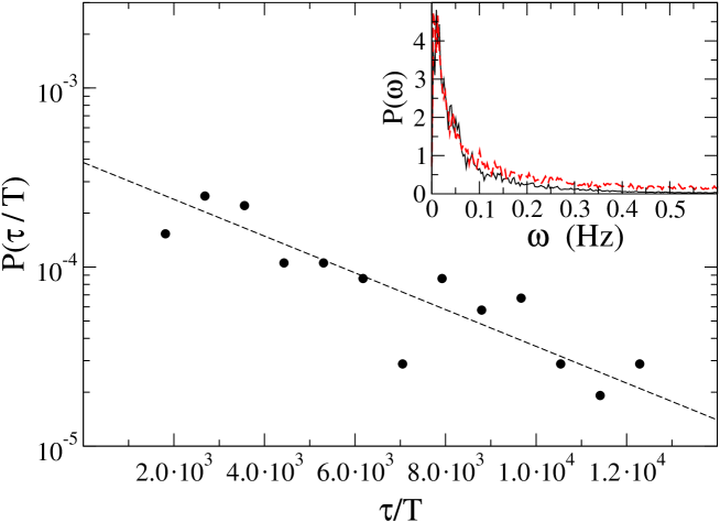
Figure 10: Probability distribution of the residence time $\tau$ for the (hardened) occupation number $N_{2}(t)$ of heavy particles. The dashed line is an exponential fit. In inset: power spectrum $P(\omega)$ of the hardened occupation number (solid line) and power spectrum of the synthetic dichotomic signal used for comparison in the text (dashed line). Simulation parameters are the same as in fig. 8.

Since the fast particles play a major role in activated processes, we computed the velocity probability distributions for the two species, in each compartment. Such distributions are shown in fig. 11, for the horizontal component of the velocity. On rescaling by the corresponding mean squared velocities, they appear to collapse on two curves, one for the “empty” compartment and another for the “full” one. The two distributions deviate from a Gaussian law and can be fitted by $f(v_{x})=A/(exp(\beta v_{x}^{\lambda})+exp(-\beta v_{x}^{\lambda}))$ (as already found in ref Daniela ) with the following values for the fitting parameters: $A_{f}=0.9,~{}\beta_{f}=1.38,~{}\lambda_{f}=1.14$ for both components in the “full” compartment and $A_{e}^{(1)}=0.8,~{}\beta_{e}^{(1)}=1.1,~{}\lambda_{e}^{(1)}=1.35$ and $A_{e}^{(2)}=1.03,~{}\beta_{e}^{(2)}=1.6,~{}\lambda_{e}^{(2)}=0.98$ for the component 1 and 2, respectively, in the “empty” one. It is interesting to observe that the exponent $\lambda$ increases with the occupation number, in agreement with the idea that high velocity tails are associated with those particle that underwent a smaller number of inter-particle collisions.

We now turn to consider the vertical temperature and density profiles (see fig. 12). The temperature profiles indicate that the kinetic temperature of the heavy species is larger than that of the light one (being the values of these two quantities dominated by the bulk of the distributions). Remarkably, in the upper region the light particles are more energetic than the heavy ones.

The density profiles show peaks at different positions for the two species, indicating that the light particles tend to stay above the heavy ones. One can also observe that the upper region, well above the top of the dividing barrier, contains mostly light grains.

For the sake of comparison, we also performed simulations of a reference system with a single compartment Meerson . For small values of $z$ the density profiles $n_{1}(z)$ and $n_{2}(z)$ result very similar to the case of the two-compartment system. For higher values of $z$, both $n_{1}(z)$ and $n_{2}(z)$ are larger than the corresponding profiles in the reference system. The local granular temperatures $T_{1}(z)$ and $T_{2}(z)$ display a similar behavior. For small values of $z$, $T_{2}(z)$ is larger that $T_{1}(z)$, because heavy grains gain a larger amount of energy when colliding with the vibrating base, but for large values of $z$ this relation is reversed: light particles are “hotter” and their temperature profile is characterized by a slower exponential decay. This is consistent with the mechanisms discussed in section V.

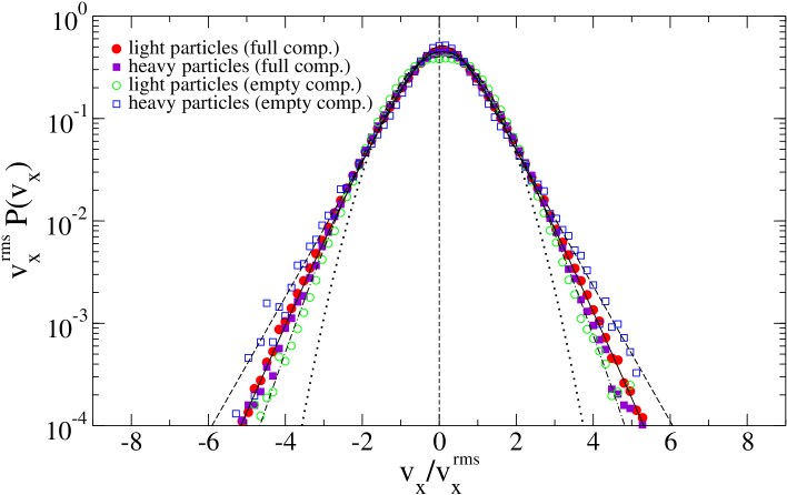
Figure 11: The rescaled velocity distribution functions $v_{x}^{rms}P(v_{x})=f(v_{x}/v_{x}^{rms})$ for horizontal velocities. The open and closed symbols correspond to the “empty” and “full” compartment, respectively. Circles and the squares correspond to the light and heavy species, respectively. The independent variable $v_{x}$ was rescaled by its mean squared value $v_{x}^{rms}$: $38.29cm/s$ (component 1) and $22.12cm/s$ (component 2) for the “full” compartment; $59.44cm/s$ (component 1) and $32.40cm/s$ (component 2) for the “empty” compartment. The solid and dash-dotted lines are the fitting laws discussed in the text, while the dotted curve is a Gaussian distribution, as an aid for the eye.

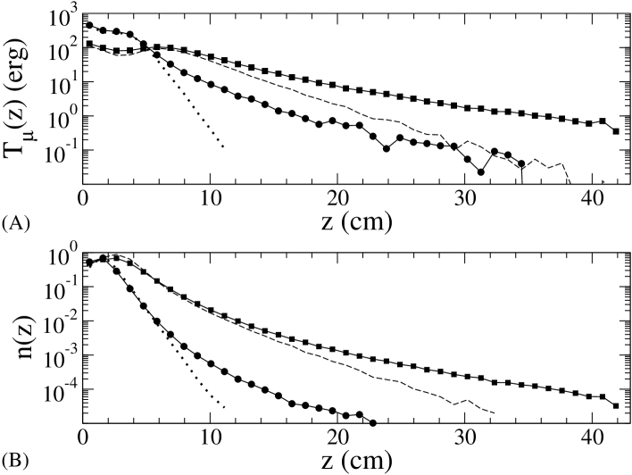
Figure 12: The granular temperature (a) and density (b) profiles versus height, for the “full” compartment. Square and circles correspond to light and heavy components, respectively, for the case with two compartments. The dashed and the dotted lines correspond to light and heavy components in the case of a single compartment.

VI Conclusions

In this paper we studied the behavior of a two-dimensional, driven, inelastic granular mixture in a compartmentalized container. Our work is hinged on two complementary approaches. The first approach consists in reducing the dynamics, by means of an appropriate coarse-graining procedure, to a simple set of non-linear coupled ordinary differential equations for the relevant observables, namely the number of particles and the average kinetic energies in each compartment. These mean-field equations are solved numerically and show the existence of three qualitatively different regimes: 1) for “low” values of the dimensionless parameter $R_{MF}$ the asymptotic state of the system is symmetric, i.e. the particles of each species are equidistributed in the two compartments; 2) for intermediate values of $R_{MF}$ the system attains a limit cycle where the populations in each compartment exhibit an oscillatory behavior, and segregation of species is observed; 3) for high values of $R_{MF}$ the system approaches an asymptotically steady state, with unequal populations in the two compartments and no segregation of species.

The second approach is a more realistic event-driven simulation with physical parameters similar to those employed in laboratory experiments. Our simulations show qualitatively similar scenarios. However, whereas in the mean-field description we find two stationary regimes, a symmetric configuration and an asymmetric one, separated by an oscillatory regime, our numerics indicate that the intermediate oscillatory “phase” is indeed a stochastic, bistable regime. In both cases, the bistability emerges only when the masses or diameters of the species are different enough. In addition to that, the typical time scale characterizing transitions in the bistable regime grows as one departs from the asymmetric phase and moves towards the symmetric phase. The mechanism that sustains such a non-stationary dynamics was explained in terms of the microscopic kinetics of a mixture of inelastic particles.

VII Acknowledgments

We wish to thank Renaud Lambiotte for sending us a preprint concerning the behavior of a granular mixture of grains of different sizes. We also thank G. Mari for having participated to the early stages of the present work. U.M.B.M. acknowledges the support of the Project Complex Systems and Many-Body Problems Cofin-MIUR 2003 prot. 2003020230.

References

- (1) Granular Gases, volume 564 of Lectures Notes in Physics, T. Pöschel and S. Luding editors, Berlin Heidelberg, Springer-Verlag (2001).
- (2) H.M. Jaeger, S.R. Nagel and R.P. Behringer, Rev. Mod. Phys. 68, 1259 (1996) and references therein.
- (3) L.P. Kadanoff, Rev. Mod. Phys. 71, 435 (1999).
- (4) H. J. Schlichting and V. Nordmeier, Math. Naturwiss. Unterr., 49, 323 (1996).
- (5) J. Eggers, Phys. Rev. Lett. 83, 5322 (1999).
- (6) R. Mikkelsen, D. van der Meer, K. van der Weele, and D. Lohse, Phys. Rev. Lett. 89, 214301 (2001).
- (7) K. van der Weele, D. van der Meer and D. Lohse, Europhys. Lett. 53, 328 (2001).
- (8) D. van der Meer, K. van der Weele and D. Lohse, Phys. Rev. Lett. 88, 174302 (2002).
- (9) D. van der Meer, K. van der Weele, and D. Lohse, Phys. Rev. E 63, 061304 (2001).
- (10) A.Lipowski and M.Droz, Phys. Rev. E 65, 031307 (2002);
- (11) A. Lipowski et al., Phys. Rev. E 66, 016118 (2002);
- (12) F. Coppex et al., Phys. Rev. E 66, 011305 (2002).
- (13) F. Cecconi, U. Marini Bettolo Marconi, A. Puglisi and A.Vulpiani, Phys. Rev. Lett. 90, 064301 (2003).
- (14) F. Cecconi, U. Marini Bettolo Marconi, A. Puglisi and F. Diotallevi, J. Chem. Phys. 121, 5125 (2004) and 120, 35 (2004).
- (15) J. Javier Brey, F. Moreno, R. García-Rojo, and M. J. Ruiz-Montero, Phys. Rev. E 65, 011305 (2002).
- (16) U. Marini Bettolo Marconi and A.Puglisi, Phys. Rev. E 68 031306 (2003).
- (17) U. Marini Bettolo Marconi and M.Conti, Phys. Rev. E 69, 011302 (2004).
- (18) D. Paolotti, C. Cattuto, U. Marini Bettolo Marconi and A. Puglisi, Granular Matter 5, 75 (2003).
- (19) T.P.C. van Noije and M.H. Ernst, Granular Matter 1, 57 (1998).
- (20) U. Marini Bettolo Marconi and A. Puglisi, Phys. Rev. E 65, 051305 (2002) and Phys. Rev. E 66, 011301 (2002).
- (21) A. Barrat and E. Trizac, Phys. Rev. E 66, 051303 (2002).
- (22) V. Garzó and J. Dufty, Phys. Rev. E 60 5706 (1999).
- (23) A. Barrat and E. Trizac, Granular Matter 4, 57 (2002).
- (24) Renaud Lambiotte and M. Salazar, preprint (2003).
- (25) U. Marini Bettolo Marconi and A.Puglisi, Phys. Rev. E 66, 011301 (2002).
- (26) D. Paolotti, A.Barrat, U. Marini Bettolo Marconi, A. Puglisi, Phys. Rev. E 61, 061304 (2004).
- (27) R. Pagnani, U.Marini Bettolo Marconi and A. Puglisi, Phys. Rev. E 66, 051304 (2002).
- (28) K. Feitosa and N. Menon, Phys. Rev. Lett. 88, 198301 (2002).
- (29) C. Cattuto and U. Marini Bettolo Marconi, Phys. Rev. Lett. 92 174502 (2004).
- (30) P. E. Krouskop and J. Talbot, Phys. Rev. E 68, 021304 (2003)
- (31) B. Meerson, T. Pöschel and Y. Bromberg, Phys. Rev. Lett. 91, 024301 (2003)