Plug Conveying in a Horizontal Tube

Abstract

Plug conveying along a horizontal tube has been investigated through simulation, using a discrete element simulation approach for the granulate particles and a pressure field approach for the gas. The result is compared with the simulation of the vertical plug conveying. The dynamics of a slug are described by porosity, velocity and force profiles. Their dependence on simulation parameters provides an overall picture of slug conveying.

1 Introduction

A quite common method for the transportation of granular media is pneumatic conveying, where grains are driven through pipes by air flow. Practical applications for pneumatic conveying can be found in food industry and in civil and chemical engineering. One distinguishes two modes of pneumatic conveying: dilute and dense phase conveying. Dilute phase conveying has been studied in much detail [1; 7; 30; 24; 21; 3; 41; 20] and is well understood. The grains are dispersed and dragged individually by the gas flow and the interaction between grains is weak. This is not true for dense phase conveying, where the particle interaction is important and where particle density waves can be observed. The behavior of these density waves depends strongly on the orientation of the tube. In vertical plug conveying, most of the particles are located in “plugs” (dense regions) that are pushed up the tube by the pressure gradient [32]. In a horizontal tube the granular medium separates into two layers, the slowly moving bed at the bottom of the pipe and the traveling ripples or the “slugs” [36; 34; 22; 45; 39], where slugs are accumulations of particles which fill up the cross-section of the tube and move quickly in the direction of transportation. Slug conveying occurs when the ratio of grain flux to gas flux is high. This transport mode is sometimes also called “plug conveying”, in this paper this term is used in reference to vertical conveying. Currently plug conveying is gaining importance in industry, because it causes less product degradation and pipeline erosion than dilute phase conveying.

Unfortunately, current models [16; 31] of slug conveying disagree even on the prediction of such basic quantities as the pressure drop and the total mass flow, and these quantities have a great impact in the industrial application. One of the reasons for the lack of valid models is that it is difficult to study slugs experimentally in a detailed way. Usually experimental setups are limited to the measurement of the local pressure drop, the total mass flux and the velocity of the slugs. The most promising experimental studies have been performed by electrical capacity tomography [14; 45; 2] and stress detectors [27; 26; 39]. Plenty of experimental research has been done on the prediction of the total pressure drop along a horizontal conveying line [9; 28; 25; 29; 22; 17] Simulational studies are handicapped by the high computational cost for solving the gas flow and the particle-particle interaction, and are therefore mostly limited to two dimensions. For the dense phase regime, simulations have been done for bubbling fluidized beds [42; 37; 15; 13; 8; 44], which show at high gas velocities the first signs of pneumatic transport [19; 40; 12], for the strand type of conveying [10; 35; 38; 43], and for slug conveying. The simulation results on slugs published by Tsuji et al [36], Tomita et al [34] and Levy [18] are discussed later in this paper.

The goal of this paper is to provide a detailed view of slugs, by using a discrete element simulation combined with a solver for the pressure drop. This approach provides access to important parameters like the porosity and velocity of the granulate and the shear stress on the wall at relatively low computational cost. Contrary to the experiments, it is possible to access these parameters with high spatial resolution and without influencing the process of transportation. Additionally to slug profiles, characteristic curves of the pressure drop and the influence of simulation parameters are measured. The simulation results are compared to the results for vertical plug conveying [32].

2 Simulation Model

Plug conveying is a special case of the two phase flow of grains and gas. It is therefore necessary to calculate the motion of both phases, as well as the interaction between them. In the following, we explain how our algorithm treats each of these problems.

2.1 Gas Algorithm

The model for the gas simulation was first introduced by McNamara and Flekkøy [23] and has been implemented for the two dimensional case to simulate the rising of bubbles within a fluidized bed. For the simulation of slug conveying we developed a three dimensional version of this algorithm.

The algorithm is based on the mass conservation of the gas and the granular medium. Conservation of grains implies that the density $\rho_{p}$ of the granular medium obeys

$$\frac{\partial{\rho_{p}}}{\partial{t}}+\vec{\nabla}\cdot(\vec{u}\rho_{p})=0,\qquad\rho_{p}=\rho_{s}(1-\phi),$$ (1)

where the specific density of the particle material is $\rho_{s}$, the porosity of the medium is $\phi$ (i.e. the fraction of the space available to the gas), and the velocity of the granulate is $\vec{u}$.

The mass conservation equation for the gas is

$$\frac{\partial{\rho_{g}}}{\partial{t}}+\vec{\nabla}\cdot(\vec{v}_{g}\rho_{g})=0,$$ (2)

where $\rho_{g}$ is the density of the gas and $\vec{v}_{g}$ its velocity. This equation can be transformed into a differential equation for the gas pressure $P$ using the ideal gas equation $\rho_{g}\propto\phi P$, together with the assumption of uniform temperature.

For small Reynolds numbers the velocity $\vec{v}_{g}$ of the gas is related to the granulate velocity $\vec{u}$ through the d’Arcy relation:

$$-\vec{\nabla}P=\frac{\eta}{\kappa(\phi)}\phi(\vec{v}_{g}-\vec{u}),$$ (3)

where $\eta$ is the dynamic viscosity of the air and $\kappa$ is the permeability of the granular medium. This relation was first given by d’Arcy in 1856 [6]. For the permeability $\kappa$ the Carman-Kozeny relation [4] was chosen, which provides a relation between the porosity $\phi$, the particle diameter $d$ and the permeability of a granular medium of monodisperse spheres,

$$\kappa(\phi)=\frac{d^{2}\phi^{3}}{180(1-\phi)^{2}}.$$ (4)

After linearizing around the normal atmospheric pressure $P_{0}$ the resulting differential equation only depends on the relative pressure $P^{\prime}$ ($P=P_{0}+P^{\prime}$), the porosity $\phi$ and the granular velocity $\vec{u}$, which can be obtained from the particle simulation, and some material constants like the viscosity $\eta$:

$$\frac{\partial{P^{\prime}}}{\partial{t}}=\frac{P_{0}}{\eta\phi}\vec{\nabla}(\kappa(\phi)\vec{\nabla}P^{\prime})-\frac{P_{0}}{\phi}\vec{\nabla}\vec{u}.$$ (5)

This differential equation can be interpreted as a diffusion equation with a diffusion constant $D=\phi\kappa(\phi)/\eta$. The equation is solved numerically, using a Crank-Nickelson approach for the discretization. Each dimension is integrated separately.

The boundary conditions are imposed by adding a term $\mp S$ on the right hand side of equation (5) at the top and the bottom of the tube, where $S\propto v_{g}P_{0}$. This mimics a constant gas flux with velocity $v_{g}$ at a pressure $P_{0}$ into and out of the tube.

2.2 Granulate Algorithm

The model for the granular medium simulates each grain individually using a discrete element simulation (DES). For the implementation of the discrete element simulation we used a version of the molecular dynamics method described by Cundall and Strack [5]. The particles are approximated by monodisperse spheres and rotations in three dimensions are taken into account.

The equation of motion for an individual particle is

$$m\ddot{\vec{x}}=m\vec{g}+\vec{F}_{c}-\frac{\vec{\nabla}P}{\rho_{s}(1-\phi)},$$ (6)

where $m$ is the mass of a particle, $\vec{g}$ the gravitation constant and $\vec{F}_{c}$ the sum over all contact forces. The last term, the drag force, is assumed to be a volume force given by the pressure drop $\vec{\nabla}P$ and the local mass density of the granular medium $\rho_{s}(1-\phi)$.

The interaction between two particles in contact is given by two force components: a normal and a tangential component with respect to the particle surface. The normal force is the sum of a repulsive elastic force (Hooke’s law) and a viscous damping. The tangential force is proportional to the minimum of the normal force (sliding Coulomb friction) and a viscous damping. The viscous damping is used when the relative surface velocity of the particles in contact is small. The same force laws are considered for the interaction between particles and the tube wall.

2.3 Gas-Grain Interaction

The simulation method uses both a continuum and a discrete element approach. While the gas algorithm uses fields, which are discretized on a cubic grid, the granulate algorithm describes discrete particles in a continuum. An interpolation is needed for the algorithms to interact. For the interpolation a tent function $F(\vec{x})$ is used:

$$F(\vec{x})=f(x)f(y)f(z),\qquad f(x)=\begin{cases}1-|x/l|,&|x/l|\leq 1,\\ 0,&1<|x/l|,\end{cases}$$ (7)

where $l$ is the grid size used for the discretization of the gas simulation.

For the gas algorithm the porosity $\phi_{j}$ and the granular velocity $\vec{u}_{j}$ must be derived from the particle positions $x_{i}$ and velocities $v_{i}$, where $i$ is the particle index and $j$ is the index of the grid node. The tent function distributes the particle properties around the particle position smoothly on the grid:

$$\phi_{j}=1-\sum_{i}F(\vec{x}_{i}-\vec{x}_{j}),\qquad\vec{u}_{j}=\frac{1}{1-\phi_{j}}\sum_{i}\vec{v}_{i}F(\vec{x}_{i}-\vec{x}_{j}),$$ (8)

where $x_{j}$ is the position of the grid point and the sum is taken over all particles.

For the computation of the drag force on a particle the pressure drop $\vec{\nabla}P_{i}$ and the porosity $\phi_{i}$ at the position of the particle are needed. These can be obtained by a linear interpolation of the fields $\vec{\nabla}P_{j}$ and $\phi_{j}$ from the gas algorithm:

$$\phi_{i}=\sum_{j}\phi_{j}F(\vec{x}_{j}-\vec{x}_{i}),\qquad\vec{\nabla}P_{i}=\sum_{j}\vec{\nabla}P_{j}F(\vec{x}_{j}-\vec{x}_{i}),$$ (9)

where the sum is taken over all grid points.

3 Simulational Results

The setup for the simulation consists of a horizontal tube of length $L_{t}=52.5\,cm$ and of internal diameter $D_{t}=7mm$. The air and the granular medium is injected at a constant mass flow rate at on end of the tube. At the beginning of a simulation the tube is empty. The default parameters were chosen to be the same as in an earlier paper [32] for vertical plug conveying. As default the mass flow rate of the granular medium is $2.49\,kg/h$. Default parameters for the particles are: diameter $d=1.4\,mm$, density $\rho_{s}=937\,kg/m^{3}$, Coulomb coefficient $\mu=0.5$ and restitution coefficient $e=0.5$. The gas volume has been discretized into 150x2x2 grid nodes, which corresponds to a grid constant of $3.5\,cm$. The gas pressure is set to $P_{0}=1013.25\,hPa$, Simulations are preformed for gas viscosities $\eta$ from $0.045\,cP$ to $0.085\,cP$ and gas flows $\dot{V}$ between $1.1\,l/min$ and $9.2\,l/min$. The gas flow is usually given by the superficial gas velocity $v_{s}=\phi v_{g}=4\dot{V}/\pi D_{t}^{2}$ [11], where $v_{g}$ is the equivalent gas velocity for an empty tube.

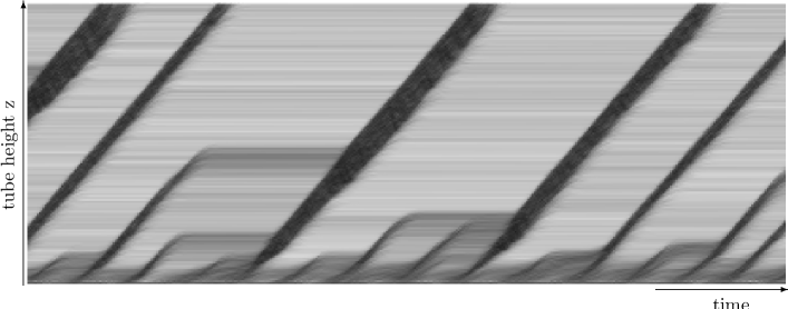
Figure 1: Spatio-temporal image of the porosity along the horizontal tube. The dark regions correspond to low porosity, light regions to high porosity. The entire tube ($52.5\,cm$) is displayed, the elapsed time is $4\,s$. Default parameters for the simulation were used; the superficial gas velocity is $1\,m/s$, the gas viscosity is $0.0673\,cP$, and the Coulomb coefficient is $0.5$. Particles are introduced at the bottom. On average 3200 particles are inside the tube, and the pressure drop is $10\,hPa/m$.

The flow in the corresponding experiment for the vertical conveying [32] is turbulent (particle $Re\approx 65$). In the simulation, an effective gas viscosity is used to account for the effect of turbulence. For an effective gas viscosity $\eta=0.0673\,cP$, a gas flow $\dot{V}=2.3\,l/min$ and a Coulomb coefficient $\mu=0.5$ slug conveying is observed as shown in figure 1. The measured pressure drop is $10\,hPa/m$, the slug velocity is $0.42\,m/s$, and the slug length is 4-8$\,cm$. An image of a corresponding slug is shown in figure 2.

Figure 2: Image of a slug corresponding to the slug conveying shown in figure 1. The direction of motion is from left to right with a superficial gas velocity of $1\,m/s$. A stretch of $11.3\,cm$ length is displayed. The slug contains about 470 particles with diameter $1.4\,mm$.

As pointed out in the introduction, some simulations of horizontal slug conveying have already been published. The horizontal transport of a slug has been studied by Tsuji et al [33]. The tube with diameter $5\,cm$ and length $80\,cm$ contained 1000 particles with a diameter of 1 cm, which the same diameter ratio as used in this study. Contrary to our simulations, the slug was created by the initial conditions, where a given range of the tube was filled with particles. Nevertheless the qualitative behavior of the particles is the same as shown in figure 2 and 17.

Tomita et al [34] assumed the slugs to be indivisible objects. The computed trajectories of the slugs are similar to the trajectories observed in our studies, however he neglects the possibility of slugs to grow or even to dissolve which is seen in our results.

Levy [18] applied a two fluid approach on the horizontal conveying. He observes the break up of a large artificially build slug into smaller slug. Such behavior is observed neither in our simulation nor in Tsuji’s.

3.1 Characteristic curves

The “characteristic curves” of a pneumatic transport system are plots of the pressure drop against the superficial gas velocity $v_{s}=\phi v_{g}$ for different mass flows of the granulate. This kind of diagram is highly dependent on the material characteristics of the tube wall and the granulate and can be used to predict the overall transport performance for given parameter sets. Such a diagram, from data of our simulation, is shown in figure 3.

Figure 3: Total pressure drop against superficial gas velocity for different granular mass flows. Plotted are characteristic curves from the simulation for the granular mass flows $2.49\,kg/h$ and $9.95\,kg/h$. For mass flow $2.49\,kg/h$ bulk transport is observed when the superficial gas velocity is below $0.25\,m/s$.

The diagram provides the typical qualitative behavior for pneumatic transport. From top left to bottom right with increasing superficial gas velocity, three regions can be distinguished. First, for small superficial gas velocities ($v_{s}<0.38\,m/s$), one has bulk transport. The tube is completely filled with granulate, so the pressure drop is high. Nevertheless the drag force on the bulk is too small to overcome the friction between the granular medium and the wall. In this case the transport comes through the enforced granular mass flow at the inlet of the tube.

For moderate velocities ($0.38\,m/s\leq v_{s}<4\,m/s$), slug conveying is observed (fig. 1). The particles injected at the inlet organize into slugs. After a short acceleration, the slugs move forward with a constant velocity. A slug always leaves particles behind it and usually maintains its length by collecting particles in front of it. A slug disintegrates when it gets too small. The particles behind the slug rest at the bottom of the tube. The amount of particles left behind a slug is independent of the slug size. Larger particle amounts left by a dissolved slug are collected by the following slug and cause it to grow. The porosity of the granular medium inside a slug is close to the minimum porosity, and the slug edges are smooth.

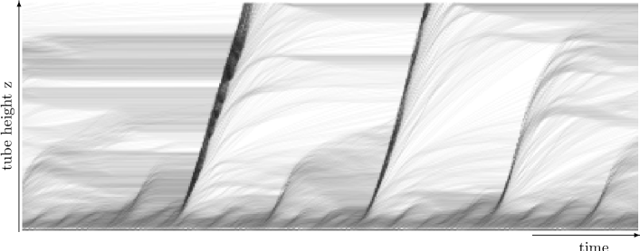
Figure 4: Spatio-temporal image of the porosity along the horizontal tube. The dark regions correspond to low porosity, light regions to high porosity. The entire tube ($52.5\,cm$) is displayed, the elapsed time is $4\,s$. A higher superficial gas velocity (4 m/s) has been used compared to the spatio-temporal image in figure 1 ($1\,m/s$). On average 1400 particles are within the tube, and the pressure drop is $10\,hPa/m$.

For high superficial gas velocities ($v_{s}>4\,m/s$) the tube is almost empty (fig. 4); in the simulation the particles are pushed out either as small slugs or as individual particles sliding on the bottom of the tube. The porosity increases with the superficial gas velocity. In this region the simulation method underestimates the pressure drop, because it does not consider the increasing drag force on single particles, which in the experiment dominates in this region. The boundaries between the described regions depend on the simulation parameters.

A nearly proportional relation is observed between the total pressure drop and the total number of particles in the tube. This can be explained by the observation that the amount of particles between the slugs is small and in the slugs most particles are densely packed at a well defined porosity. Through d’Arcy’s law, the total pressure drop depends linearly on the tube length filled with this porosity, since the pressure drop on the granulate between the slugs is negligible and causes only a small deviation. At high gas velocities this is no longer true, because the plugs no longer contain the majority of the particles.

In the following, the dependence of the pressure drop on the mass flux of the granulate, the air viscosity $\eta$, the atmospheric pressure $P_{0}$ and the Coulomb coefficient $\mu$ is discussed. For the parameter studies the superficial gas velocity has been fixed to $1\,m/s$. For higher velocities the sensitivity to the parameter values decreases.

Figure 5: Dependence of the pressure drop on the mass flux of the granulate at a superficial gas velocity $1\,m/s$.

As one can see in figure 5 the pressure drop increases linearly with mass flux of the granulate. The increase in the pressure drop is associated with an increase of the number of slugs within the tube.

The gas flow can be influenced by changing the atmospheric pressure $P_{0}$ or the diffusion constant $D$. An increase in background pressure $P_{0}$ combined with an increase in superficial velocity leaves the pressure drop unchanged. This can be deduced directly from equation (5) by noting that both terms on the right hand side are proportional to $P_{0}$.

Figure 6: Dependence of the pressure drop on the dynamic viscosity $\eta$ of the gas at a superficial gas velocity $1\,m/s$.

The diffusion constant $D\propto d^{2}/\eta$ can be changed through the particle diameter $d$ and the viscosity $\eta$. Therefore it is sufficient to analyze the parameter space for the viscosity at a constant diameter as shown in figure 6. The pressure drop is decreasing with increasing viscosity.

The parameter of the particle simulation with most influence on the transport of the granular medium is the Coulomb coefficient $\mu$. The restitution coefficient has only a small effect, except when it is unrealistically large.

Figure 7: Dependence of the pressure drop on the Coulomb coefficient $\mu$. The superficial gas velocity is $1\,m/s$. For low Coulomb coefficients ($\mu<0.1$) even small particle groups are able to slide within the tube, so slugs do not occur.

As one can see in figure 7 the pressure drop increases with $\mu$. For low Coulomb coefficients ($\mu<0.1$) the injected particles are sliding individually along the tube with accelerating speed. As most of the tube is empty, the total pressure drop is small. As $\mu$ increases, the particles start first to slide as one layer. Then the particle layer gets slower and thicker and therefore causes an higher pressure drop. At a Coulomb coefficient of $\mu=0.1$, a peak in the pressure drop coincides with the transition from the conveying by a sliding particle layer to slug conveying. Slugs first occur when the cross-section of the tube is filled locally somewhere along the tube. They are more efficient in transporting particles, therefore the pressure drop first decreases until a pure slug conveying is reached ($0.1<\mu<0.15$). For higher coefficients ($\mu>0.15$) the slugs become slower due to the growing friction and cause therefore a rising pressure drop.

3.2 Slug statistics

The spatio-temporal image of the porosity along the horizontal tube (fig. 1) provides a rough picture of slugs and their movement along the tube. A statistical approach is necessary to get more precise values. Properties of interest are the porosity and the granular velocity within a slug, the slug length, and their dependence on the horizontal position $x$ of the slug within the tube. To get some average values for the porosity and the granular velocity, the tube was segmented into horizontal slices of length $3.5\,mm$. For each slice the average porosity and granular velocity was computed every $0.01\,s$. The contribution of a particle was weighed by the volume occupied by that particle within a given slice.

The resulting vertical porosity was used to identify slugs. Every region with a porosity lower than 0.6 is defined to belong to a slug.

Figure 8: Number of slugs per time as a function of tube position $x$. The corresponding spatio-temporal image is shown in figure 1. The total tube length is $52.5\,cm$, and default parameters are used. The data is averaged over $22.5\,s$.

Figure 8 shows the slug rate, or number of slugs per time as a function of the position along the tube. At the inlet of the tube the incoming granular medium fragments into many small slugs. Even though their velocity is low, the resulting slug rate is high. As can be seen in figure 1, many slugs dissolve along the tube, therefore the slug rate decreases. Most slugs dissolve within the first $0.3\,m$ along the tube. Beyond $x=0.3\,m$ the number of slugs remains stable until they leave the system.

For each slug, the center of mass, the minimal porosity, the maximal granular velocity and the slug length have been computed.

Figure 9: Minimal porosity in slugs at tube position $x$, corresponding to the slug rate shown in figure 8. The bars denote the uncertainty of the average, and the dotted lines indicate the width of the distribution; at each value of $x$, half of the observed slugs have a porosity lying between the upper and the lower dotted lines. The slug porosity decreases when the granulate enters the tube ($x<0.2\,m$) and increases when it leaves the tube ($x>0.45\,m$).

Figure 9 shows the minimum slug porosity as a function of the horizontal position $x$ of a slug. At each value of $x$, the mean porosity and its uncertainty (standard deviation divided by the square root of the number of slugs) were calculated. These quantities are shown by the bars in figure 9. To show the distribution of porosity about the mean, the two dotted lines were added. At each position $x$, half of the slugs have a porosity lying between these two lines. The same analysis was carried out for the data in Figures 10 and 11. As one can see in figure 9 at the left of the graph, the granular medium is inserted at the inlet of the tube with a porosity of 0.57. From there the porosity decreases quickly to about 0.47 at a height $x=0.2\,m$ and then remains almost constant until $x=0.45\,m$. At the end of the tube ($x>0.45\,m$) the porosity increases again until the grains leave the simulation space at $x=0.525\,m$.

Figure 10: Maximal granular velocity in slugs at tube position $x$, corresponding to the slug rate shown in figure 8. The bars and dotted lines have the same meaning as in figure 9. The granular velocity saturates in the middle of the tube, the increase of the granular velocity at the beginning and at the end of the tube is due to the boundary effects described in figure 9.

Figure 10 shows the corresponding particle velocity. The change in porosity comes along with an increase of the granular velocity within the slugs. The granulate is inserted with an initial velocity of $0.04\,m/s$. The granular velocity saturates to a final velocity ($0.3\,m/s$) at a position of $0.2\,m$. Starting at about $0.45\,m$, the granular medium accelerates until the grains leave the tube.

An explanation for the constant slug velocity in the middle of the tube can be derived using the balance equation for the forces on a slug:

$$F=-F_{c}+\alpha(\phi)(v_{g}-u).$$ (10)

where $F_{c}$ is the force on the slug due to the friction with the wall. The last term $\alpha(\phi)(v_{g}-u)$ is the drag force on the slug, which is proportional to the relative velocity between the particles and the gas within the slug. At the middle of the tube the porosity of the slug $\phi$ is constant. On small time scales the gas velocity $v_{g}$ can be assumed constant. Only the drag force depends on the granular velocity $u$ through equation (3). For a certain granular velocity the drag force balances the friction forces, and thus $u$ remains constant. The solution is stable under small fluctuations in $u$.

Figure 11: Mean slug length at tube position $x$, corresponding to the slug rate shown in figure 8. The bars and dotted lines have the same meaning as in figure 9. The average slug length increases along the tube, consistent with the decrease in the slug rate (fig. 8).

Figure 11 shows the mean slug length along the tube. The average slug length increases along the tube, due to the collection of particles of dissolved slugs by the following ones. Beyond $x=0.3\,m$ a stable slug length is reached. The increase of the slug length combined with the decrease of the number of slugs per time (fig. 8) conserves the mass flux of the granulate.

As can one seen from Figs. 9, 10 and 11, the boundary condition at $x=0.525\,m$ affects only a small region close to the end of the tube. In vertical plug conveying, this boundary region is much larger. This difference arises because the grains between the plugs or slugs have different behaviors. In vertical conveying, particles are falling downwards, so that when a plug is removed at the top of the tube, the flux of particles onto the next plug is reduced shortly thereafter. On the other hand, in horizontal conveying, the grains between the slugs are simply lying on the bottom of the tube. When a slug is removed at the end of the tube, this information is not transmitted to the next plug. The succeeding slug is only influenced by the thickness of the particle layer left behind. Another consequence of this difference is that, contrary to the vertical conveying, the distance between slugs has no effect on their interaction.

The slug profiles (Fig. 12-16) indicate that the slugs only interact through the thickness of the particle layer left behind them. Defining everything with a porosity lower then 0.6 as belonging to a slug, the interaction range with the particle layer is of the size of the slug length.

The diagrams in figures 9 to 11 imply that there is a typical porosity, granular velocity and length of slugs and a characteristic slug profile for a given position along the tube exists. In the following averaged vertical and radial profiles of slugs at the position of $0.26\,m$ are discussed. To get some sensible profiles, slugs with length and granular velocity close to the mean values ($L_{p}=0.05\pm 0.03\,m$, $u=0.29\pm 0.1\,m/s$) were selected.

3.3 Horizontal slug profiles

While in experiments recognizing and measuring parameters for global slug conveying are rather simple, the measurement of profiles for individual slugs remains a nearly impossible task. So one of the reasons for simulating slug conveying is to provide a detailed picture of what happens within a slug, and how parameters like porosity, granular velocity, or shear stress change along the slug.

Figure 12 to 16 present averages of different quantities over six slugs. These slugs were taken from the middle of the tube $x=0.26\,m$ with granular velocity $0.29\pm 0.1\,m/s$ and slug length $0.05\pm 0.03\,m$. The coordinate $\Delta x$ denotes the relative vertical position along the tube with respect to the center of mass.

Figure 12: Horizontal porosity profile along an averaged slug, containing about 470 particles, positioned at the middle of the tube. The profile was averaged over six slugs with granular velocity $0.29\pm 0.1\,m/s$ and slug length $0.05\pm 0.03\,m$. The data belong to the simulation displayed in figure 1. The horizontal axis denotes the relative horizontal position $\Delta x$ along the tube with respect to the center of mass. The horizontal position is given in multiples of the particle diameter $d=1.4\,mm$.

The porosity profile of the slugs is shown in Figure 12. At the front side of the slug, on the right hand side of figure 12, the porosity decreases from 85% to $50\%$. In the middle the porosity of the slug remains almost constant, and increases at the backside of the slug. The high porosity before and after the slug corresponds to a dense particle layer at the bottom of the tube and a region devoid of particles above this layer (fig. 17).

Figure 13 displays the velocity profile of the granular medium for the slugs shown in Figure 12. One can distinguish four different regions: Ahead of the slug ($\Delta x/d\geq 30$), the high porosity corresponds to the few particles resting at the bottom of the tube, averaged over the cross-section of the tube.

Figure 13: Averaged velocity of the granular medium along the averaged slug of figure 12. Inside the region around the slug ($\Delta x/d<-40$ & $\Delta x/d>30$) the granular medium is moving forward, outside it is resting.

These particles originate from the backside of a preceding slug. The friction outweighs the drag force on the particles. At the front side of the slug ($10\geq\Delta x/d>30$), the particles accelerate, as they are pushed by the low porosity region. In the following, this region at the front of the slug will be called collision region. Inside the slug, where the porosity settles to a low value, the average granulate velocity is almost constant ($|\Delta x/d|>10$). At the back side ($-10<\Delta x/d\leq-40$) of the slug the granular medium slows down until it rests again. Thus the slug is always loosing material at the back side. This region will be called disintegration region.

Figure 14: Forces in the direction of motion acting on particles along the averaged slug in figure 12. Interparticle forces and friction are summed up and displayed as particle force. The drag force corresponds to the pressure drop of the gas. Outside of the slug ($\Delta x/d<-40$ & $\Delta x/d>30$) the particle force is zero. The fluctuations in the particle force ($x/d\approx 20$) are strongest in the collision region, where the moving particles within the slug collide with the resting particles before the slug.

The trajectory of a single particle through the slug can be sketched by a snapshot of the horizontal forces acting on it. Figure 14 displays the drag force $F_{d}$ and the sum over the interparticle and friction forces on a particle (here called particle forces) $F_{p}$. These forces are averaged over the cross-section of the tube. Before entering the slug, the drag force on the particles is small, because the air is able to pass above the particles. The large fluctuations in the particle force arise when the moving particles within the slug collide with the resting particles before the slug. Within this region the particles are piled up, until the cross-section of the tube is completely filled. In the slug the drag force and the friction force balance each other. Behind the slug, the drag force becomes negligible and the particles are slowed down by the friction with the wall until they come to rest.

Figure 15: Stress between the wall and the granular medium along the averaged slug of figure 12. The low wall stress before and after the slug corresponds to the weight of the layer of particles resting at the bottom of the tube, which is given by the dotted curve.

The normal wall stress corresponding to the slug in Figure 12 is shown in Figure 15. In horizontal conveying the normal wall stress is the sum of the normal interparticle forces and the weight of the particles. The low wall stress before and after the slug corresponds to the weight of the layer of particles left behind by the slugs. Higher wall stresses are produced by the slug including the collision and disintegration region. The wall stress increases within the collision region and then decreases in the disintegration region. As one can see, the wall stresses are much higher than can be accounted for by the weight of the material. Therefore, the particle in the slug must have a high granular temperature.

Figure 16: Granular temperature along the averaged slug of figure 12. The granular temperature increases rapidly at the front of the slug. Due to the large damping ($e=0.5$) the granular temperature is dissipated. Behind the center of the slug the temperature decreases linearly until it vanishes behind the slug.

Figure 16 shows the granular temperature along a slug. The granular temperature is the average kinetic energy of the particles minus the kinetic energy of the motion of their center of mass. The granular temperature rises rapidly in the collision region. Due to the high damping ($e=0.5$) these temperatures decrease along the slug and vanish behind the slug.

3.4 Cross-sections of a slug

In horizontal slug conveying, the radial symmetry of the system is broken by the gravitational force. The particles tend to segregate and settle on the bottom of the tube (fig. 17). In the middle of the slug, the complete cross-section of the tube is filled with particles. At the bottom of the tube, the particles form layers along the wall.

Figure 17: Cross-sections of volume fraction of particles at half tube length. The pictures were taken at a frame rate of $100\,Hz$. From left to right an interval of $0.2\,s$ is displayed. The greyscale from black to white corresponds to porosities from 100 to 0%.

Figure 18: Vertical velocity profile through the slug shown in figure 17

Before the slug the particles are resting (fig. 18). At the front side of the slug the particles gain velocity in direction of motion. This velocity decreases behind the slug until the particles are again resting.

Figure 19: Vertical velocity profile through the slug shown in figure 17

Within the slug the lower particle layers are slower than the upper ones, as shown in figure 19. The particle layer at the bottom of the tube is slowed down due to the high friction with the wall. The uppermost particles within the tube, moving freely between the upper tube wall and the other particles below, have the highest velocity.

4 Comparison of horizontal and vertical transport

The same simulation method as used for horizontal conveying has also been applied to vertical conveying. A parameter study and a detailed analysis of the plugs for the vertical plug conveying has been published separately [32], with tube dimensions and default parameters for the particles and the gas being identical.

(a)

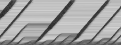
(b)

Figure 20: Spatio-temporal images of the porosity along the tube for (a) the horizontal and (b) the vertical plug conveying. All the parameters, except for the direction of gravity are the same in both simulations.

As expected from experiments, plug conveying is observed in both the horizontal and the vertical cases. However the details of the flow patterns and the quantitative properties are different.

The most conspicuous difference between the flow patterns is that in the horizontal transport most slugs dissolve while traveling along the tube. Succeeding slugs grown through collecting the remnants of preceding slugs. Contrary to the vertical transport, there is a final slug length. After reaching certain length slugs do not dissolve any more. In the vertical transport the growth of plugs comes through the merging of smaller plugs. Vertical plugs are slower ($0.17\,m/s$) then in horizontal transport ($0.3\,m/s$), as the drag force acting on the plugs is partly compensated by the gravitational force. The initial number of plugs at the beginning of the tube is lower in the horizontal conveying, because the minimal number of particles needed to fill up the cross-section of the tube is higher.

Another feature also observed in experiments is that in horizontal transport the particles between the slugs form a resting layer at the bottom of the tube. In vertical case the corresponding particles are accelerating downwards, the impact of these particles on a succeeding plug is considerable higher then in the horizontal case.

The characteristic curves show some significant differences between the transport modes. Generally the pressure drop in the tube filled with plugs for the vertical transport is about four times higher than for the horizontal transport. The additional pressure drop is needed to carry the plugs against the gravitational force. The qualitative behavior of the pressure drop with the superficial gas velocity and the viscosity is the same for both cases. The pressure drop in slug conveying decreases about six times more rapidly with increasing superficial gas velocity. It is decreasing less with increasing gas viscosity. In both cases the pressure drop shows a linear dependency on the mass flux of the granulate. An increase of the mass flux results in more plugs along the tube.

(a)

(b)

Figure 21: Dependency of the pressure drop on the Coulomb coefficient for (a) the horizontal and (b) the vertical plug conveying.

The dependence on friction is different between horizontal and vertical conveying, as can be seen from figure 21. While in the horizontal case for low Coulomb coefficients $\mu<0.05$ the granular material is transported as single particles, which are rolling on the bottom of the tube, in the vertical case the granular material is transported as plugs even with no friction at all. Here the pressure drop in the horizontal case is considerable lower then anywhere else. A peak in the pressure drop ($\mu=0.1$) for the horizontal transport denotes transition from the transport of particle layers at the bottom of the tube by sliding or rolling to slug transport. On the other hand, the pressure drop increases monotonically for all values of $\mu$ in vertical conveying. For high Coulomb coefficients ($\mu>0.3$) in the horizontal case, the pressure drop increases almost linearly. In the vertical case, the increase of the pressure drop is not linear. As one can see from Fig 21b, there is a change in slope near $\mu=0.5$. This change seems to be associated with the appearance of sticking plugs.

A detailed view on the plug profiles exhibits more differences. Contrary to the vertical plugs, horizontal slugs have smooth boundaries due to the slopes at the ends of the slug. Within the vertical plug a slightly lower porosity is reached (vert. 0.47, horiz. 0.49). The slugs do not have a constant granular velocity. The average granular velocity along the horizontal slug increases from both sides until the middle of the slug. Also a shearing of particle layers within the slug is observed, where the upper particles are the fastest. The granular velocity is aligned in the direction of transport all along the tube, which is not true for the particles between the plugs in the vertical case. In the vertical case only a small difference in the granular velocity of the radial particle layers is observed, within the plug these layers have a constant velocity.

The magnitude of the maximal wall stress within a plug is of the same order for horizontal and vertical transport. The increase and decrease of the stress is spread over the whole plug length. The biggest difference in the examined plug profiles is found for the granular temperature. While in the vertical transport high granular temperatures are limited to the upper front of the plugs and vanish rapidly within the plug due to damping, in the horizontal transport the temperature decreases linearly along the slug and reaches zero far behind the slug (fig. 16).

5 Conclusion

In this paper, a simple model [23] with coupled grain and gas flow has been applied to pneumatic transport. The implementation is three-dimensional; rotation and Coulomb friction are taken into account. The fluxes of gas and grains are set by the boundary conditions. Slug conveying is observed. The simulation used for slug statistics and profiles contained on average 3200 particles in a tube of length $0.525\,m$ and diameter $7\,mm$. We simulated $22.5\,s$; during this time 27 different slugs were observed at the middle of tube, each with about 500 particles. Additionally 24 simulations were performed to obtain the characteristic curves.

As for the vertical plug conveying [32], an effective viscosity $\eta$ and an effective friction $\mu$ has been introduced. The effective viscosity reflects the increased momentum transport in the gas due to the turbulent flow around the grains. The effective friction reflects the complex interplay between sliding, rolling and static friction. Large numbers of slugs could be studied, and their porosity, velocity, and size were measured as functions of height.

The simulation results imply that the slug formation at the beginning of the tube occurs spontaneously. There is a well defined preferred velocity of the slugs, which is independent of the slug size and the tube length. The average slug length increases along the tube due to the collection of particles resting between the slugs. The results also show that boundary effects at the bottom and the top of the tube have to be taken into account. For the experimental parameters, the influence of the boundaries is limited to a distance of $0.05\,m$, which is about the size of a slug in the middle of the tube. Slugs accelerate in these boundary regions. The acceleration at the upper boundary arises due to the lack of resting grains before the slug. This implies that the momentum transfer to accelerate these grains can not be neglected. A model of slug conveying must take this into account, as these grains reduce the slug velocity.

Also a detailed view of an average slug was presented. In contrast to experimental setups, we are not limited to measure the slug properties only at few locations. Experimental results usually provide the slug properties as a function of time at a given position along the tube, with the disadvantage that the slug profile is distorted by the relative motion of granulate along the slug. The vertical profiles were given for porosity, granular velocity, interparticle and drag forces, wall stress and granular temperature. In the experiment, these parameters usually are not accessible along the whole tube.

Additionally cross-section profiles are given at high resolution. The results show that the grains are ordered into horizontal layers. These layers have different velocities with a fluctuation 3.5 times larger than the mean value. A shearing of the particle layers is observed, where the lowest layers are the slowest and the highest layers are the fastest.

A comparison of the horizontal slug conveying with the vertical conveying shows that the flow patterns, the characteristic curves, and the plugs differ. While in vertical conveying small plugs typically merge to bigger plugs, the small slugs in horizontal conveying typically dissolve. In the vertical case plugs are influenced by the distance to preceding plugs, which is not true for the horizontal conveying. Generally the total pressure drop in the vertical case is about four times higher as in the horizontal case. In horizontal conveying an additional conveying mode is observed for low friction, where particles slide or roll at the bottom of the tube. In vertical conveying a sticking of plugs within the tube is found for high friction or low superficial velocities. The radial symmetry of the plug is broken for horizontal transport, which comes along with a shearing of vertical particle layers.

In conclusion, the model presented here is a useful tool for investigating slug conveying. It is fast and flexible enough to make parameter studies on full featured slug conveying and provides at the same time access to the slug properties at the level of grains. It can obtain both characteristic curves and slug profiles. Future optimizations and faster computers will permit this model to be applied to industrial-sized systems. As a next step, angular periodic boundary conditions will be applied to vertical transport. In this way, simulations at higher tube diameters will be possible.