Phonon Coherence and New Set of Sidebands in Phonon-Assisted Photoluminescence

Abstract

We investigate excitonic polaron states comprising a local exciton and phonons in the longitudinal optical (LO) mode by solving the Schrödinger equation. We derive an exact expression for the ground state (GS), which includes multi-phonon components with coefficients satisfying the Huang-Rhys factors. The recombination of GS and excited polaron states gives one set of sidebands in photoluminescence (PL): the multi-phonon components in the GS produce the Stokes lines and the zero-phonon components in the excited states produce the anti-Stokes lines. By introducing the mixing of the LO mode and environal phonon modes, the exciton will also couple with the latter, and the resultant polaron states result in another set of phonon sidebands. This set has a zero-phonon line higher and wider than that of the first set due to the tremendous number of the environal modes. The energy spacing between the zero-phonon lines of the first and second sets is proved to be the binding energy of the GS state. The common exciton origin of these two sets can be further verified by a characteristic Fano lineshape induced by the coherence in the mixing of the LO and the environal modes.

It has been recognized that the interactions of excitons with phonons in light-emitting materials lead to a number of interesting effects in optical properties, such as the phonon sidebands in photoluminescence (PL) spectra, the exciton dephasing and self-trapping 1 ; 2 ; 3 ; 4 ; 5 ; a5 ; 6 ; 7 . Theoretically, the sideband structures caused by electron-phonon interactions for local excitons at deep centers were investigated using the Huang-Rhys model 8 ; 9 ; 10 . In these theories, an adiabatic approximation is applied to separate the degrees of freedom of excitons and phonons. One set of Stokes lines (SLs) in PL, observed in the experiments, has been very successfully explained by the theories. However, there are some features in the experimental spectra associated with the interactions of excitons and phonons, such as complicated structure containing more than one set of phonon sidebands, anti-Stokes lines (ASLs), and Fano-like lineshape, seemingly beyond the adiabatic approximation. Recently, the fabrication of nanostructures has renewed the study of this field, as the confinement in quantum dots much enhances the interaction between carriers and phonons. Such an enhancement has been experimentally observed aa1 ; aa2 . Fomin et al. have proposed a nonadiabatic approach to interpret the unusual phonon sidebands observed in quantum dots dev . Verzelen et al. have indicated that the exciton-phonon bound states as a whole, called excitonic polarons, and the decaying of their phonon components into phonon thermostat have to be put under consideration in cases of strong exciton-phonon interactions 11 .

In this Letter, we present a unified theory beyond the adiabatic approximation to explain complicated structures of phonon sidebands in PL. The exact eigenstates and eigenenergies of excitonic polarons are obtained by solving the Schrödinger equation of an exciton interacting with LO mode. The obtained ground state (GS) contains multi-phonon components with coefficients strictly satisfying the Huang-Rhys factors, which gives the SLs including a ZPL. Meanwhile the zero-phonon components of the excited states can produce the ASLs. These SLs and ASLs form one set of sidebands. By introducing the mixing of LO mode and environal modes, another set emerges. The energy shift between two sets is determined by the strength of exciton-LO phonon coupling, and the coherence in the mode mixing results in specific Fano-like lineshape.

First, let us consider the interaction between an exciton and a LO mode

$$H=\epsilon_{0}a^{{\dagger}}a+\hbar\omega_{0}b^{{\dagger}}_{0}b_{0}+V_{0}a^{{\dagger}}a(b^{{\dagger}}_{0}+b_{0}),$$ (1)

where $a$ and $b_{0}$ are annihilation operators for exciton and for LO phonon, $\epsilon_{0}$ and $\hbar\omega_{0}$ are their energies, respectively, and $V_{0}$ is the coupling strength between exciton and phonon. Here we regard the exciton as one quasiparticle, supposing that it has a large binding energy.

For Hamiltonian (1), the $m$th eigen-wavefunctions can be written as

$$\Psi_{m}=\sum_{n}c_{m;n}\frac{a^{{\dagger}}(b^{{\dagger}}_{0})^{n}}{\sqrt{n!}}|0\rangle,$$ (2)

where $n$ is the number of phonons of the LO mode in the corresponding component, $|0\rangle$ is the vacuum, and the coefficients satisfy the following iteration relations

$$[E_{m}-(\epsilon_{0}+n\hbar\omega_{0})]c_{m;n}=V_{0}\sqrt{n}c_{m;n-1}+V_{0}\sqrt{n+1}c_{m;n+1}.$$ (3)

For the GS ($m=0$), $E_{0}$ is below $\epsilon_{0}$, and coefficients are related with each other by

$$c_{0;1}=\frac{(E_{0}-\epsilon_{0})c_{0;0}}{V_{0}},$$

$$c_{0;2}=\frac{(E_{0}-\epsilon_{0}-\hbar\omega_{0})c_{0;1}-V_{0}c_{0;0}}{\sqrt{2}V_{0}}$$

$$=\frac{(E_{0}-\epsilon_{0})c_{0;1}}{\sqrt{2}V_{0}}+\frac{-\hbar\omega_{0}(c_{0;1}/c_{0;0})-V_{0}}{\sqrt{2}V_{0}}c_{0;0},$$

$$\ldots,$$

$$c_{0;n+1}=\frac{(E_{0}-\epsilon_{0}-n\hbar\omega_{0})c_{0;n}-V_{0}\sqrt{n}c_{0;n-1}}{\sqrt{n+1}V_{0}}$$

$$=\frac{(E_{0}-\epsilon_{0})c_{0;n}}{\sqrt{n+1}V_{0}}+\frac{-n\hbar\omega_{0}(c_{0;n}/c_{0;n-1})-V_{0}\sqrt{n}}{\sqrt{n+1}V_{0}}c_{0;n-1}.$$ (4)

From these relations, we can find the exact expressions of the GS energy

$$E_{0}=\epsilon_{0}-\Delta_{0}$$ (5)

with $\Delta_{0}\equiv\frac{V_{0}^{2}}{\hbar\omega_{0}}$ being the binding energy of the excitonic polaron, and the coefficients

$$c_{0;n}=\frac{(-1)^{n}S^{n/2}}{e^{S/2}\sqrt{n!}},$$ (6)

with $S$ being the Huang-Rhys factor $S=\frac{V_{0}^{2}}{\hbar^{2}\omega_{0}^{2}}\equiv\frac{\Delta_{0}}{\hbar\omega_{0}}.$ Considering that the $n$th component in GS $\Psi_{m=0}$ is associated with $n$ phonons, $|c_{0;n}|^{2}$ gives the intensity of a phonon sideband at energy $E_{0}-n\hbar\omega_{0}$. This is as predicted by the Huang-Rhys theory.

Figure 1: Several low-lying eigenenergies $E_{m}$ as functions of $n_{\text{max}}$, the maximum number of phonons included in the calculation. $\epsilon_{0}=3.366$eV, $\hbar\omega_{0}=0.069068$eV, (a) $V_{0}=0.01$eV, (b) $V_{0}=0.03$eV, (c) $V_{0}=0.05$eV, (d) $V_{0}=0.08$eV. The dotted lines represent the corresponding values of $\epsilon_{0}+m\hbar\omega_{0}$ for comparison.

For excited states $\Psi_{m}$ with $m>0$, exact analytical expressions can not be obtained in this way. However, from a numerical diagonalization shown in Fig. 1 one can see that for both cases of weak and strong coupling the eigenvalues can be expressed as

$$E_{m}=\epsilon_{0}+m\hbar\omega_{0}-\Delta_{0}.$$ (7)

From this the coefficients in the eigenfunctions can be obtained by the following iteration relations

$$c_{m;n+1}=-\frac{c_{m;n}}{\sqrt{n+1}V_{0}D_{m;n}},\text{ for }n=0,1,2,\ldots,$$ (8)

where

$$D_{m;n+1}=\frac{1}{\Delta_{0}-(m-n-1)\hbar\omega_{0}-(n+1)V_{0}^{2}D_{m;n}},$$

with the initial value

$$D_{m;0}=\frac{1}{\Delta_{0}-m\hbar\omega_{0}},$$

and by the normalization. Although the eigenenergy of state $\Psi_{m}$ with $m>0$ is higher than $E_{0}$, it should have a finite occupation rate as long as the photon energy of the excitation laser is high enough 15 . In order to calculate the PL spectrum of the polaron states, we must know the population of each state. For simplicity, we assume that all the states with energies less than the laser energy $E_{\text{laser}}$ have the same occupation rate. The intensity of PL at photon energy $\epsilon$ is proportional to

$$\rho(\epsilon)=\sum_{m}\sum_{n}|c_{m;n}|^{2}\theta(E_{\text{laser}}-E_{m})\delta(\epsilon-E_{m}+n\hbar\omega_{0}).$$ (9)

The luminescence peaks produced by the GS $\Psi_{0}$ consist of a ZPL at energy $E_{0}=\epsilon_{0}-\Delta_{0}$ and a number of SLs at energies $E_{0}-n\hbar\omega_{0}$. This ZPL originates from the zero-phonon component ($c_{0;0}$) of the GS state while the remaining lines are from the components ($c_{0;n>0}$) with more than one phonon. The intensities of the SLs relative to the ZPL follow a Poisson distribution predicted by the Huang-Rhys theory. Other eigenstates $\Psi_{m>0}$ will produce complex sideband structures, which is not dealt with in the Huang-Rhys theory. Radiative recombination of these states will intensify the ZPL peak by accompanying with simultaneous emission of $m$ LO phonons. When they emit $n>m$ phonons in the radiative recombination, the intensity of the SL at $E_{m}-n\hbar\omega_{0}$ will be enhanced. Meanwhile, the component $c_{m;n<m}$ of state $\Psi_{m}$ may produce the ASL peak at $E_{m}-n\hbar\omega_{0}$ above the ZPL, together with the emission of $n(<m)$ phonons. The relative intensity of this ASL is $\rho_{m;m-n}/\rho_{m;m}=\frac{S^{n}(m)!}{n!^{2}(m-n)!}$.

It is known that besides LO mode, there are a large number of bath phonon modes in solids. Although these bath modes do not directly interact with the exciton, they may have crucial influence on phonon components of the polaron states. This influence can be accounted for using the following Hamiltonian of the mode mixing

$$H_{1}=\sum_{\lambda}g(b^{{\dagger}}_{0}b_{\lambda}+\text{H.c.})+\sum_{\lambda}\hbar\omega_{\lambda}(b^{{\dagger}}_{\lambda}b_{\lambda}+\frac{1}{2}),$$ (10)

where $\lambda$ is the mode index of bath phonons, and $g$ is the strength of the mixing. For simplicity, $g$ is assumed to be the same for all bath modes and the dispersion relation $\omega_{\lambda}$ is continuous with a constant density of states between energies 0 and $W$. For a pure harmonic phonon system without exciton, the mixing terms should vanish as all the phonon modes are orthogonal to each other. The formation of the excitonic polaron states, however, violates the orthogonality between the LO and bath modes, and thus creates the mixing terms. It is this mixing that makes the LO phonons in the polaron states $\Psi_{m}$ decays into the continuum of bath modes. From Hamiltonian (10), the orthogonal modes become

$$b_{l}=\frac{\hbar\omega_{l}-\hbar\omega_{0}}{\sqrt{g^{2}+(\hbar\omega_{0}-\hbar\omega_{l})^{2}}}b_{\lambda}+\frac{g}{\sqrt{g^{2}+(\hbar\omega_{0}-\hbar\omega_{l})^{2}}}b_{0},$$ (11)

with frequency $\omega_{l}$ determined by solving the equation

$$\hbar\omega_{l}=\hbar\omega_{0}+\sum_{\lambda}\frac{g^{2}}{\hbar\omega_{l}-\hbar\omega_{\lambda}}.$$ (12)

The resultant set of orthogonal modes $\{l\}$ will couples with the exciton at a strength

$$V_{l}=\frac{g}{\sqrt{g^{2}+(\hbar\omega_{0}-\hbar\omega_{l})^{2}}}V_{0}.$$ (13)

Figure 2 shows the phonon frequency dependence of $V_{l}$. It can be seen that most of the modes $\{l\}$ are still weakly coupled to the exciton except for those modes with frequencies $\omega_{l}\sim\omega_{0}$. As mentioned earlier, this results in not only the broadening of the peaks in the first set but also the creation of the second set of the phonon sidebands.

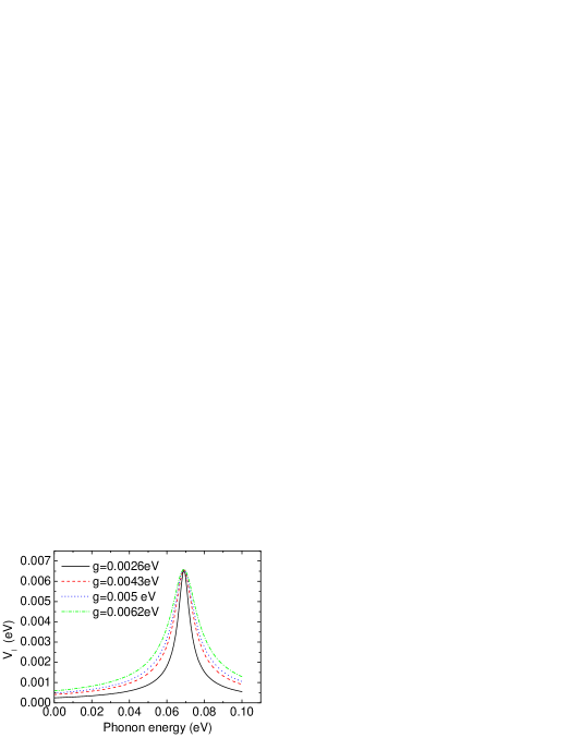
Figure 2: Coupling strength $V_{l}$ as a function of phonon frequency.

To give a clarification, we can divide the modes $\{l\}$ into two groups: $P_{1}$ includes modes with $\omega_{l}\sim\omega_{0}$ which strongly couple with the exciton; $P_{2}$ includes the remaining modes weakly coupled to the exciton. Because the modes in $P_{1}$ with frequencies in the vicinity of $\omega_{0}$ have coupling strength of about $V_{0}$ with the exciton, the formed polaron states will produce the first set of phonon sidebands including broadened ZPL, SLs and ASLs, as already discussed above. It should be noted that the ZPL is centered at the GS eigenenergy $E_{0}$ which lows with increasing $g$ due to an increase of the mode number in group $P_{1}$ as seen from Fig. 2. Now we turn to discuss the modes in $P_{2}$. For a mode $l$ in this group, it has a weak coupling with the exciton, i.e., $V_{l}\sim 0$, so the binding energy of the relevant polaron state is approaching zero. In other words, the eigenenergy of the polaron state is very close to the bare exciton energy $\epsilon_{0}$. Thus, the ZPL produced by the zero-phonon component in this state almost located at $\epsilon_{0}$, higher than the ZPL of the first set by an energy about $\varepsilon_{0}-E_{0}$. The intensity of the ZPL in the second set should be much stronger than that of the ZPL in the first set since the ZPL intensity is proportional to the number of involved phonon modes. Because of the evident dispersion of the bath modes in group $P_{2}$, it can be expected that the ZPL of the second set is wider than that of the first set. The energetic position of the one-phonon sideband in the second set ranges from $\epsilon_{0}$ (the ZPL position) to $\epsilon_{0}-W$. The transition probability of this sideband is found to be

$$p_{\,l0;1}\propto\frac{(\hbar\omega_{l}-\hbar\omega_{0}+g)^{2}}{g^{2}+(\hbar\omega_{0}-\hbar\omega_{l})^{2}}.$$ (14)

From Eq. (14), it can be easily known that $p_{l0;1}$ reaches its maximum value for $\hbar\omega_{l}=\hbar\omega_{0}+g$ and the minimum for $\hbar\omega_{l}=\hbar\omega_{0}-g$. When the phonon frequency is increased from $\hbar\omega_{0}-g$ to $\hbar\omega_{0}+g$ the intensity of the sideband rapidly increases. However, as the phonon frequency is further increased over $\hbar\omega_{0}+g$ the sideband intensity slowly decreases. This results in a typical Fano asymmetric lineshape. As a matter of fact, one can rewrite Eq. (14) into a standard Fano lineshape function $\alpha_{l}=(\tilde{\epsilon}+1)^{2}/(\tilde{\epsilon}^{2}+1)$ with $\tilde{\epsilon}=(\hbar\omega_{l}-\hbar\omega_{0})/g$. Here the Fano asymmetry parameter is the unity 16 . Since the mixing between LO-mode and $\lambda$-mode (which forms the $l$ mode components in the polaron states, illustrated in Eq. (11)), introduced by $H_{1}$, is coherent, an interference between the optical transitions associated with the two phonon components in the $l$ mode will occur. That is the origin of Fano interference in the phonon-assisted luminescence.

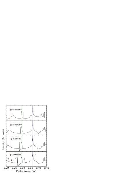
Figure 3: Relative intensity as a function of photon energy when $H_{1}$ is included. In the simulation 1000 modes uniformly distributed in a band from 0 to 0.1eV are included. $V_{0}=0.0078$eV. Other parameters are the same as those in Fig. 1.

By diagonalizing the whole Hamiltonian $H+H_{1}$, one can calculate the PL spectrum by

$$\rho(\epsilon)=\sum_{m}\sum_{\{n_{l}\}}|c_{m;\{n_{l}\}}|^{2}\left(\prod_{l}\alpha_{l}^{n_{l}}\right)\theta(E_{\text{laser}}-E_{m})$$

$$\times\delta(\epsilon-E_{m}+\sum_{l}n_{l}\hbar\omega_{l}),$$ (15)

where $E_{m}$ and $c_{m;\{n_{l}\}}$ are eigenenergy and eigenfunction of the whole Hamiltonian. In Fig. 3, we plot the PL spectrum obtained from a numerical calculation. As expected, there are two ZPL peaks, 0’ and 0, belonging to the first and second set, respectively. In each set, there are several SLs and ASLs. The SLs are red-shifted from their corresponding ZPL by integer times $\hbar\omega_{0}$ while the energy distances of the ASLs from the ZPL are not integer times $\hbar\omega_{0}$. It is because that the energy positions of the ASLs are determined by energies of the excited polaron states whose energies are not exactly higher than the GS energy by integer times $\hbar\omega_{0}$. The Fano interference features are partially smeared by the summation in Eq. (15), but they can still be seen near some peaks. These results catch the essential nature observed in experiments [13, ].

In a summary, by reconsidering the exciton-phonon interaction and decaying of LO phonons we can conclude that there are two sets of phonon assisted peaks: one is from excitonic polaron states of the phonon modes with frequencies $\omega_{l}\sim\omega_{0}$, and the other is from polaron states of the remaining bath phonon modes. The latter set was not properly considered in previous theories and was usually assigned to be the first set because it may include the strongest “ZPL” peak. The common exciton origin of these two sets of phonon sidebands can be further verified by the characteristic energy difference between them determined by the exciton-LO phonon coupling strength, and by the specific Fano lineshape reflecting the coherence in the phonon mode mixing. Together with the experimental observation, the present theory may give a new and better understanding of the complicated structures in the phonon-assisted luminescence spectrum.

Acknowledgments This work was supported in HK by HK RGC CERG Grant (No. HKU 7036/03P), in Nanjing by National Foundation of Natural Science in China Grant Nos. 60276005 and 10474033, and by the China State Key Projects of Basic Research (G20000683).

References

- (1) A. S. Davydov, Theory of Molecular Excitons, Plenum, New York, 1971.
- (2) R. S. Knox, in Solid State Physics, Suppl. 5, edited by F. Seitz and D. Turnball, Academic, New York, 1963.
- (3) Polarons and Excitons. edited by C. G. Kuper and G. D. Whitfield, Plenum, New York, 1963.
- (4) E. Peter, J. Hours, P. Senellart, A. Vasanelli, A. Cavanna, J. Bloch, and J. M. Gérard, Phys. Rev. B. 69, 041307(R) (2004).
- (5) P. Borri, W. Langbein, U. Woggon, M. Schwab, M. Bayer, S. Fafard, Z. Wasilewski, and P. Hawrylak, Phys. Rev. Lett. 91, 267401 (2003).
- (6) U. Hohenester and G. Stadler, Phys. Rev. Lett. 92, 196801 (2004).
- (7) L. D. Landau, Phys. Z. Sowjetunion 3, 664 (1933).
- (8) T. G. Castner and W. Käzig, J. Phys. Chem. Solids, 3, 178 (1957).
- (9) K. Huang and A. Rhys, Proc. Roy. Soc. (London) A204, 406, (1950).
- (10) C. B. Duke and G. D. Mahan, Phys. Rev. 139, A1965 (1965).
- (11) B. Segall and G. D. Mahan, Phys. Rev. 171, 935 (1968).
- (12) V. Jungnickel and F. Henneberger, J. Lumin. 70, 238 (1996).
- (13) M. Bissiri, G. Baldassarri, H. von Högersthal, A. S. Bhatti, M. Capizzi, A. Frova, P. Frigeri, and S. Franchi, Phys. Rev. B 62, 4642 (2000).
- (14) V. M. Fomin, V. N. Gladilin, J. T. Devreese, E. P. Pokatilov, S. N. Balaban, and S. N. Klimin, Phys. Rev. B 57, 2415 (1998); V. N. Gladilin, S. N. Klimin, V. M. Fomin, and J. T. Devreese, ibid. 69, 155325 (2004); V. A. Fonoberov, E. P. Pokatilov, V. M. Fomin, and J. T. Devreese, Phys. Rev. Lett. 92, 127402 (2004).
- (15) O. Verzelen, R. Ferreira, and G. Bastard, Phys. Rev. Lett. 88, 146803 (2002).
- (16) H. Zhao, S. Moehl, S. Wachter, and H. Kalt, Appl. Phys. Lett. 80, 1391 (2002).
- (17) U. Fano, Phys. Rev. 124, 1866 (1961).
- (18) S. J. Xu, S. J. Xiong, and S. L. Shi, preprint.