Structure and stability of Mott-insulator shells of bosons trapped in an optical lattice

Abstract

We consider the feasibility of creating a phase of neutral bosonic atoms in which multiple Mott-insulating states coexist in a shell structure and propose an experiment to spatially resolve such a structure. This spatially-inhomogeneous phase of bosons, arising from the interplay between the confining potential and the short-ranged repulsion, has been previously predicted. While the Mott-insulator phase has been observed in an atomic gas, the spatial structure of this phase in the presence of an inhomogeneous potential has not yet been directly probed. In this paper, we give a simple recipe for creating a structure with any desired number of shells, and explore the stability of the structure under typical experimental conditions. The stability analysis gives some constraints on how successfully these states can be employed for quantum information experiments. The experimental probe we propose for observing this phase exploits transitions between two species of bosons, induced by applying a frequency-swept, oscillatory magnetic field. We present the expected experimental signatures of this probe, and show that they reflect the underlying Mott configuration for large lattice potential depth.

I Introduction

Recent experimental results involving quantum degenerate atom gases trapped in optical lattices have stimulated interest from the perspectives of condensed matter and quantum information science. Ultra-cold atoms confined in an optical lattice are predicted to display a rich variety of quantum phases (see Jaksch98 ; Kuklov04a , for example). The ability to precisely control the physical parameters of this system enables probing a vast range of related fundamental physics including quantum phase transitions, the behavior of collective excitations in the quantum regime, and the physics of defects. The properties of these phases may permit new applications, such as neutral atom quantum computing or quantum simulation Jane03 .

Neutral bosons trapped in optical lattices can exhibit complex spatial configurations of co-existing superfluid and Mott-insulator phases Jaksch98 . There have been detailed studies of the superfluid to Mott-insulator phase transition in the atomic system using techniques such as quantum Monte Carlo simulation and mean-field theory (see Oosten01 ; Kashurnikov02 ; Batrouni02 ; Wessel04 for examples). In this paper we offer a practical and simple recipe for realizing specific Mott-insulator configurations and we study the limitations posed by realistic experimental conditions. Motivated by proposals for using the Mott-insulator state to initialize a fiducial state for neutral atom quantum computing Rabl03 ; Brennen03a , we focus on the tight-binding regime where inter-site tunneling is suppressed. We formulate a straightforward method, primarily using counting arguments, for obtaining the constraints on lattice parameters that yield states of definite spatially varying occupation number.

The effects of finite temperature, tunneling, and dissipation in a periodic potential have been studied in the literature LeggettRMP ; Sethna ; HanggiTalknerBorkovec90 . Atomic systems are a unique tool for studying outstanding questions regarding these phenomena. Furthermore, deviations from the zero-temperature and tightly-bound ground state will have an important impact on potential applications using atoms trapped in a lattice. We investigate processes which disturb the stability of the Mott-insulator ground state and estimate their influence for characteristic experimental conditions. Specifically, we initiate an analysis of the emergence of superfluid order when there is a finite but small degree of tunneling and we study thermally-activated defects and their dynamics. Our work is not meant to be an exhaustive study of stability. Instead, we take the first steps toward addressing these considerations and point to existing literature from the condensed matter community appropriate to the atomic system.

To complement our theoretical work, we propose a set of experiments using microwave spectroscopy to map out the spatial structure of the bosonic states hosted in the optical lattice. The proposed techniques can identify Mott-insulator states with any site occupation number and resolve the spatial distribution of sites with different occupation number. We view this method as intermediate between less general techniques Rom04 and high-resolution direct imaging Vala03 which will be necessary for long-term development of neutral atom quantum computing.

This paper focuses on experimental parameters similar to those first used to observe the superfluid to Mott-insulator phase transition in an atomic gas Greiner02a . We consider using ⁸⁷Rb atoms confined in an optical lattice formed from three pairs of intersecting laser beams with wavelength $\lambda=850$ nm. The resulting lattice has cubic three-dimensional symmetry with lattice spacing $a=\lambda/2$. The effect of an external potential that changes over many lattice sites, formed from magnetic or optical fields, is included. The lattice depth is $V_{0}=30E_{\rm R}$, where the recoil energy $E_{\rm R}$ is approximately $h\times 3.7$ kHz ($h$ is Plank’s constant). The resulting tunneling strength between sites is of order $w\approx h\times 10$ Hz. The on-site interaction $U$ between particles can be changed by changing $V_{0}$ or using a Feshbach resonance. For $V_{0}=30E_{\rm R}$ and at zero magnetic bias field, $U\approx h\times 2.5$ kHz.

The outline of this paper is as follows. In Sec. II, we present a scheme for realizing Mott-insulator configurations with specified occupation numbers. In Sec. III, we address the stability of the Mott-insulator configuration, in particular, against superfluid order and defect formation. In Sec. IV, we describe experiments that exploit microwave transitions between hyperfine states to probe the Mott-insulator structure. We conclude with a summary of our discussions in Sec. V.

II Co-existence of Mott-insulator phases

In this section, we describe an optical lattice in a radially symmetric geometry that permits the co-existence of concentric Mott-insulating regions with differing occupation numbers. We derive the constraints on lattice parameters necessary for this co-existence. In contrast to previous work Jaksch98 , we employ counting arguments to describe the spatial structure of the Mott-insulator state, which allows us to consider a general spatial geometry. Our starting point is the Bose-Hubbard Hamiltonian FisherWeichmanGrinsteinFisher89 ; Jaksch98

$$\hat{H} = \left\{\sum_{i}\left[V(\textbf{r}_{i})-\mu\right]\hat{n}_{i}+\frac{U}{2}\sum_{i}\hat{n}_{i}\left(\hat{n}_{i}-1\right)\right\}$$ (1)

$$-w\sum_{\langle i,j\rangle}\left(\hat{b}_{i}^{{\dagger}}\hat{b}_{j}+\hat{b}_{j}^{{\dagger}}\hat{b}_{i}\right)\equiv\hat{H}_{0}+\hat{W}$$

where $\mu$ is the chemical potential, $V(\textbf{r}_{i})$ is the value of the external confining potential at site $i$ of the optical lattice (at the point $\textbf{r}_{i}$ in space), $\hat{b}^{{\dagger}}_{i}$ and $\hat{b}_{i}$ are the boson creation and destruction operators at site $i$, $\hat{n}_{i}\equiv\hat{b}_{i}^{{\dagger}}\hat{b}_{i}$ is the number operator for bosons on site $i$, $U$ is the on-site interaction energy between two bosons, and $\hat{W}$ represents the tunneling that tends to delocalize bosons, with $w$ being the tunneling matrix element for bosons between nearest neighbor sites $\langle i,j\rangle$ on the lattice.

In this section, we concentrate on the limit $w/U=0$ where tunneling is negligible and $\hat{H}\rightarrow\hat{H}_{0}$. (For small tunneling $w/U$, $\hat{W}$ can be treated as a perturbation; we return to this in a later section.) The sites are decoupled in this limit and the Hamiltonian, $\hat{H}_{0}$, is diagonalized by the set of states with specific occupation number on each site $|n\rangle_{i}={\big{(}b_{i}^{\dagger}\big{)}^{n_{i}}}|0\rangle_{i}/{\sqrt{n_{i}!}}$. For a given $|n\rangle_{i}$, the energy is $E_{n}=-\tilde{\mu}\,n+\frac{U}{2}(n^{2}-n)$, where $\tilde{\mu}$ is an “effective” local chemical potential $\tilde{\mu}\equiv\mu-V(r)$. The occupation number $n$ that minimizes the energy is determined by ${\partial E_{n}}/{\partial n}=0=-\tilde{\mu}-\frac{U}{2}(2n-1)$, which gives $n=\frac{\tilde{\mu}}{U}+\frac{1}{2}$. Since $n$ can take on only integer values, the minimization condition becomes

$$n-1<\frac{\tilde{\mu}}{U}<n,\ \ \mbox{$E_{n}$ is minimum}.$$ (2)

The state with $n$ bosons, which we refer to as the $n$ Mott-insulator state, is an incompressible Mott-insulator phase.

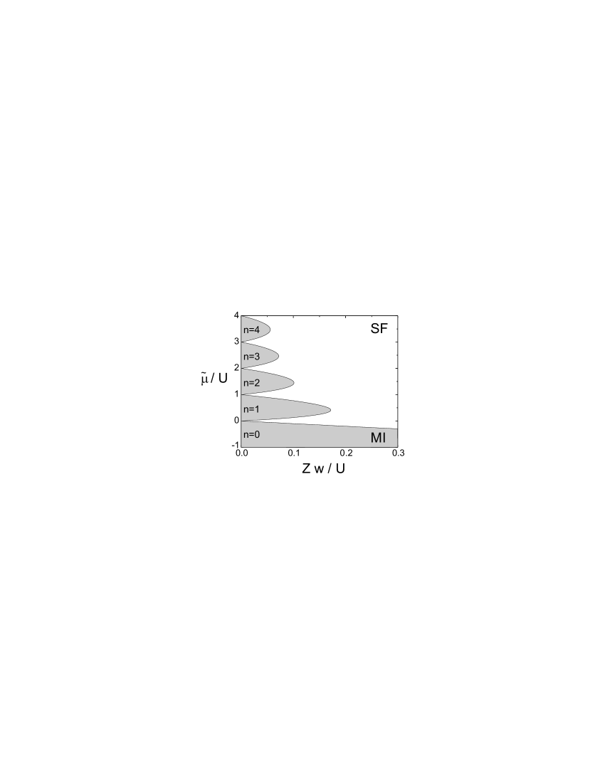
Figure 1: The mean-field phase diagram for the Bose-Hubbard Hamiltonian at first perturbative order in $w/U$. Here, $\tilde{\mu}\equiv\mu-V(r)$, as described in the text, and $Z$ is the coordination number of the lattice ($Z=6$ for the three-dimensional cubic lattice under consideration here). The shaded regions are Mott insulating with the indicated number of bosons per site, $n$. The white regions are superfluid. Notice that the superfluid regions at integer values of $\tilde{\mu}$ extend all the way to zero tunneling ($w/U=0$). While the exact location of the boundaries between superfluid and Mott regions at finite tunneling is different at higher orders in perturbation theory, the qualitative features of the phase diagram persist Sachdev .

With finite but small tunneling ($w/U\neq 0$), the regions where $\tilde{\mu}/U$ is nearly an integer become superfluid, leading to the well-known phase diagram shown in Fig. 1. At finite temperature but negligible tunneling, all Mott-insulator phases are replaced by normal fluid phases of bosons which display thermally activated hopping FisherWeichmanGrinsteinFisher89 . At suitably low temperatures $kT\ll\Delta E$, where $\Delta E$ is the excitation energy for adding or removing a particle, the system is most likely to be found in its ground state, which is the situation we consider in this section; we discuss the effects of finite temperature and tunneling in subsequent sections.

For a spatially varying external potential $V(\textbf{r})$ , and therefore spatially varying effective chemical potential $\tilde{\mu}$, the system can have co-existing regions of different Mott-insulator states Jaksch98 ; GreinerThesis . If the external potential is spherically symmetric and of the form $V(r)=\alpha r^{\xi}$, then $\tilde{\mu}$ is the largest at $r=0$ and decreases for increasing $r$. Note that the arguments in this section can be extended for more general potentials lacking spherical symmetry. In the $w/U=0$ limit, the site occupation number $m$ at the center is determined by the condition $m-1<{\mu}/U<m$, where the chemical potential $\mu$ is determined by the total number of particles $N$. The number of bosons per site changes by one at each radius where $[\mu-V(\textbf{r})]/U$ is an integer, leading to a shell structure. The radii for the boundaries, as illustrated in Fig.2, are given by $R_{n}=\left([\mu-nU]/{\alpha}\right)^{1/\xi}$ ($n=0,1,\dots,m-1$), where the $n$-th Mott-insulator state lies between $R_{n}$ and $R_{n-1}$. This shell structure is established by the competition between interaction and potential energy. The edge of the occupied lattice is defined by the outermost boundary of the Mott-insulator states where the occupation drops to zero

$$R_{0}=\left(\frac{\mu}{\alpha}\right)^{1/\xi}.$$ (3)

All other radii can be expressed in terms of $R_{0}$:

$$R_{n}=R_{0}[1-n/(\mu/U)]^{1/\xi}.$$ (4)

Figure 2: Illustration of the bounding values of $r$ for an spherically-symmetric confining potential centered at $r=0$ which supports shells of Mott-insulator phases.

For a given interaction energy $U$ and total number of bosons $N$, co-existence of a total of $m$ Mott shells will occur only for a specific range of the parameter $\alpha$. We find that range as follows: the chemical potential $\mu$ is determined via the global constraint

$$N=\sum_{i}n_{i}(\mu).$$ (5)

If the spacing between sites in the optical lattice, $a$, is small compared with $R_{0}$, we can approximate each Mott region by a three-dimensional continuous spherical shell with inner radius $R_{n}$, outer radius $R_{n-1}$ and uniform density $n/a^{3}$. In this continuum limit,

$$N = \frac{1}{a^{3}}\int n(r)d^{3}r$$ (6)

$$= \frac{4\pi}{3a^{3}}\left(R_{0}^{3}+R_{1}^{3}+R_{2}^{3}+\ldots R_{m-1}^{3}\right)$$ (7)

$$= \frac{4\pi}{3a^{3}}R_{0}^{3}\sum_{n=0}^{m-1}\left(\frac{\mu-nU}{\alpha}\right)^{3/\xi}.$$ (8)

With some rearrangement, we arrive at the condition

$$x\equiv\frac{3Na^{3}}{4\pi}\left(\frac{\alpha}{U}\right)^{3/\xi}=\sum_{n=0}^{m-1}(\mu/U-n)^{3/\xi}.$$ (9)

Because $m-1<\mu/U<m$, we can obtain from Eq. (9) the upper and lower bounds on $x(\mu/U)$ necessary to realize a shell structure with any desired maximum site occupancy $m$. For example, for $\xi=2$ (a harmonic external potential),

$$1 < \frac{3Na^{3}}{4\pi}\left(\frac{\alpha}{U}\right)^{3/2}<3.82,\ \ m=2,$$ (10)

$$3.83 < \frac{3Na^{3}}{4\pi}\left(\frac{\alpha}{U}\right)^{3/2}<9.03,\ \ m=3.$$ (11)

As an example, we consider the experimental parameters detailed in the introduction and $N=10^{6}$ atoms. To support three Mott-insulator shells in a harmonic trap $V(r)=\alpha r^{2}$ the curvature of the trap needs to satisfy the constraint $h\times 8.8$ Hz$/\mu\mbox{m}^{2}<\alpha<h\times 15.6$ Hz$/\mu\mbox{m}^{2}$. For a typical value in this range, for instance, $\mu/U=2.5$ (and hence $\alpha=h\times 12.1$ Hz$/\mu\mbox{m}^{2}$), Eq. (3) and Eq. (4) show that the size of the entire Mott-insulator structure is given by $R_{0}=22.8~{}\mu$m, and that the radii separating the three Mott shells are $R_{1}=17.6~{}\mu$m and $R_{2}=10.2~{}\mu$m.

In this section, we have shown how the spatial structure of the Mott-insulator ground state in the absence of tunneling depends on a limited number of experimental parameters. Based on counting arguments, we have derived a series of constraints on these parameters for realizing a shell structure with a specific core occupancy.

III Stability of the Mott-insulator phases

The stability of the Mott structure is relevant to experiments probing the physics described in section II. Of particular practical concern is the elimination of number fluctuations when using the Mott-insulator state as a fiducial state for neutral atom quantum information experiments. Several proposals suggest creating the Mott-insulator state followed by a purification scheme to prepare a well-defined state with one atom per lattice site Rabl03 ; Brennen03a . These schemes cannot eliminate sites that are initially vacant and suffer inaccuracy when number fluctuations become large.

Deviations from the nested Mott-insulator shell structure will be driven by finite tunneling between lattice sites and finite temperature. The dynamic evolution of the system is a result of the complex interplay between the Bose-Hubbard Hamiltonian, dissipation, and finite temperature. While a complete study of stability is beyond the scope of this paper, we summarize the effects of tunneling and finite temperature and provide estimates relevant to a typical experiment.

We assume that the lattice parameters described in the previous section determine the initial conditions for the bosons and that the lattice potential is free of imperfections. In the following sections, we first discuss global deviations from the Mott-insulator structure coming from the tendency to form superfluid regions. We show that the effects of superfluidity can be made negligible in the optical lattice. We then discuss the local fluctuations caused by “particle” and “hole” (p-h) defects in the Mott-insulator structure. We analyze the emergence and dynamics of p-h defects at finite temperature and tunneling.

III.1 Superfluidity

In principle, even the smallest amount of tunneling can alter the Mott-insulator phase. At finite tunneling, the natural source of instability is the formation of superfluid regions. As shown in the phase diagram of Fig. 1, the system is particularly susceptible to forming regions of superfluid at the boundaries between Mott states of different occupation number. For a specfic set of values for the tunneling $w$, interaction energy $U$ and external potential curvature $\alpha$, we can estimate the size of the superfluid regions formed between Mott phases. The Mott states remain relatively robust against delocalization if the expected thickness of the superfluid shells is less than a lattice spacing.

To estimate the size of the superfluid region at $T=0$, we invoke a mean-field treatment that decouples lattice sites even in the presence of tunneling Sachdev . To summarize the treatment, the effective Hamiltonian takes the form

$$H_{{\rm MF}}=\sum_{i}\Big{[}-\tilde{\mu}_{i}\hat{n}_{i}+\frac{U}{2}\hat{n}_{i}(\hat{n}_{i}-1)-\Psi_{B}\hat{b}_{i}^{{\dagger}}-\Psi^{*}_{B}\,\hat{b}_{i}\Big{]}.$$ (12)

Here $\Psi_{B}=Zw\langle b\rangle$ is related to the superfluid order parameter and is obtained self-consistently, with $Z$ being the co-ordination number (the number of nearest neighbors per site). Terms involving $\Psi_{B}$ and $\Psi^{*}_{B}$ can be treated as a perturbation to the Mott-insulator states $|n\rangle$. To second order in $\Psi_{B}$, the perturbed eigenstates at a single site are

$$|\Psi_{n}\rangle = |n\rangle+\Psi_{B}\alpha_{1}^{+}\sqrt{n+1}|n+1\rangle+\Psi_{B}^{*}\alpha_{1}^{-}\sqrt{n}|n-1\rangle$$ (13)

$$+\Psi_{B}^{2}\alpha_{2}^{+}|n+2\rangle+(\Psi_{B}^{*})^{2}\alpha_{2}^{-}|n-2\rangle,$$

where $\alpha^{\pm}_{1/2}$ are functions of $n$, $\mu$ and $U$. The energies are shifted to

$$\tilde{E}_{n}=E_{n}+\chi_{n}\big{|}\Psi_{B}\big{|}^{2}+{\cal O}\Big{(}\big{|}\Psi_{B}\big{|}^{4}\Big{)},$$ (14)

where $E_{n}$ is the energy of the unperturbed Mott state $|n\rangle$, and $\chi_{n}=\frac{n+1}{Un-\mu}+\frac{n}{\mu-U(n-1)}$. Self-consistently minimizing $\tilde{E}_{n_{0}}-Zw\langle b\rangle\langle b^{{\dagger}}\rangle-\langle b\rangle\Psi_{B}^{*}-\langle b^{\dagger}\rangle\Psi_{B}=E_{n_{0}}+\rho\big{|}\Psi_{B}\big{|}^{2}+{\cal O}\Big{(}\big{|}\Psi_{B}\big{|}^{4}\Big{)}$ determines $\Psi_{B}$. Here, $n_{0}$ is the Mott ground state occupation number appropriate for $\tilde{\mu}$. The superfluid boundaries are determined by the sign of $\rho(\mu,w,U)$; $\langle b\rangle$ has a non-zero expectation value where $\rho(\mu,w,U)$ is negative. We have to first non-vanishing order in $Zw/U$, $\rho=\chi_{n_{0}}(\mu/U)[1-Zw\chi_{n_{0}}(\mu/U)]$ with

$$\chi_{n_{0}}=\frac{n_{n_{0}}(\mu/U)+1}{Un_{0}(\mu/U)-\mu}+\frac{n_{0}(\mu/U)}{\mu-U[n_{0}(\mu/U)-1]}.$$ (15)

The superfluid boundary satisfies the condition $1-Zw\chi_{n_{0}}=0$. For fixed tunneling, this determines the boundary values of the effective chemical potential along each Mott-insulator lobe in Fig. 1. For $Zw/U\ll 1$, we have for the effective chemical potential at the upper ($\tilde{\mu}^{+}_{n_{0}}$) and lower ($\tilde{\mu}^{-}_{n_{0}}$) boundaries of the $n_{0}$ Mott-insulator lobe

$$\frac{\tilde{\mu}_{n_{0}}^{+}}{U}\approx n_{0}(1-Zw/U),\ \ \frac{\tilde{\mu}_{n_{0}}^{-}}{U}\approx(n_{0}-1)(1+Zw/U).$$ (16)

Eq. (16) can be used to determine the radii $r_{n_{0}-1}^{+}$ and $r_{n_{0}}^{-}$ between which superfluidity will exist in the continuum limit. If the distance between the radii where superfluidity can exist is smaller than a lattice spacing ($\Delta r=r_{n_{0}-1}^{+}-r_{n_{0}}^{-}<a$), then number fluctuations due to superfluid tendencies are expected to be negligible.

As an example, we again consider the experimental situation detailed in the introduction with a harmonic external potential and $\mu/U=2.5$. The thickness of the superfluid between the $n_{0}=1$ and $n_{0}=2$ Mott-insulator states is $\Delta r_{1-2}\approx 0.82\sqrt{{U}/{\alpha}}\,{Zw/U}$. Using the value $\alpha\approx h\times 12.1$ Hz$/\mu\mbox{m}^{2}$ from the previous section, we obtain $\Delta r_{1-2}\approx 0.07~{}\mu$m and $\Delta r_{2-3}\approx 0.24~{}\mu$m, which is smaller than the lattice spacing $a\approx 0.43~{}\mu$m. Therefore, for this specific case, no superfluid regions will exist. Eq. (16) could also be used to determine the experimental parameters leading to the existence of superfluid shells, which may be of fundamental interest in and of themselves.

III.2 Defects

While global instabilities coming from a tendency for the bosons to condense can be made negligible, local instabilities can still permeate the Mott-insulator structure in the form of defects. In this section, we discuss two types of local excitations — isolated defects where a site has an extra particle or one less (hole) compared with the Mott-insulator ground state, and excitations where a particle has hopped to a neighboring site and leaves behind a hole. The former, which we call “site-defects” can arise from random removal of atoms from the lattice, for example by heating from spontaneous emission driven by the lattice light or by collisions with room-temperature residual gas molecules in the vacuum system. We refer to the latter as “particle-hole” (p-h) excitations and these are natural perturbations to the Mott-insulator ground state. Site-defects can also arise when components of p-h excitations (due to finite temperature or imperfect adiabatic transfer) that were present during initial loading of the Bose-Einstein condensate into the lattice become widely separated.

In the following discussion, we first consider the energy gap associated with these excitations; the energy gap plays a key role in the statics and dynamics of defects. We then study the static perturbative effects of p-h excitations on the Mott-insulator state in the presence of finite tunneling. Next, we consider the dynamics of defects within the framework of a toy two-site model. We comment on defect dynamics over the entire system and on the effects of dissipation. Finally, we discuss the role of finite temperature.

Energy Gap In the Mott-insulator ground state at zero tunneling, the functional $E(n)=-\tilde{\mu}n+\frac{U}{2}n(n-1)$ is minimized at each site. The energy gap associated with single site defects is $\Delta E^{+}=E_{n_{0}+1}-E_{n_{0}}=-\tilde{\mu}+Un_{0}$ for the addition of an extra particle and $\Delta E^{-}=E_{n_{0}-1}-E_{n_{0}}=\tilde{\mu}-U(n_{0}-1)$ for the removal of a particle (addition of a hole), where $n_{0}$ is the ground-state occupation number. Since $n_{0}-1<\frac{\tilde{\mu}}{U}<n_{0}$, $\Delta E^{\pm}$ is positive and of order $U$ in the bulk of the system. Close to Mott boundaries, though, the energy gap becomes arbitrarily small as $\frac{\tilde{\mu}}{U}$ approaches either $n_{0}$ or $n_{0}-1$. Because of the underlying lattice and inhomogeneous confining potential, however, the energy cost for a site defect rarely vanishes: there is always a change in potential energy $\Delta V$ over a lattice spacing and it is unlikely for a boundary to exactly coincide with a lattice site. For the experimental parameters detailed in the introduction, $V_{i}=(h\times 12.1~{}{\rm Hz}/{\mu{\rm m}^{2}})r_{i}^{2}$, we have $\Delta V=h\times 181$ Hz ($h\times 104$ Hz) at the boundary $R_{1}=17.6~{}\mu{\rm m}$ ($R_{2}=10.2~{}\mu{\rm m}$).

The energy cost for a p-h excitation in the bulk is

$$E_{i}^{{\rm hop}}(n_{0})\equiv\Delta E_{i}^{+}+\Delta E_{i+1}^{-}=\Delta V_{i}+U,$$ (17)

where $i$ is a site index, $\Delta V_{i}=V_{i}-V_{i+1}$, and $V_{i}$ is the on-site potential energy from the confining potential. For a particle hopping across a boundary between a Mott-insulator $n_{0}$ phase on site $i$ and $n_{0}-1$ phase on site $i+1$, the energy cost is

$$E_{i}^{{\rm hop}}(n_{0}\downarrow) \equiv \Delta E_{i}^{-}(n_{0})+\Delta E_{i+1}^{+}(n_{0}-1)=\Delta V,$$

$$E_{i}^{{\rm hop}}(n_{0}\uparrow) \equiv \Delta E_{i}^{+}(n_{0})+\Delta E_{i+1}^{-}(n_{0}-1)$$ (18)

$$= 2U-\Delta V,$$

The symbol $\downarrow$ denotes hopping from an $n_{0}$ to an $n_{0}-1$ Mott-insulator state and $\uparrow$ denotes the reverse process. The most favorable p-h excitation therefore involves a particle hopping across a Mott-insulator boundary from higher to lower occupation.

Finite Tunneling - Statics:

At small tunneling ($w\ll U$), corrections to the $w=0$ Mott-insulator ground state $|\psi_{0}\rangle$ can be written in terms of p-h excitations provided that $w\ll E_{i}^{\rm hop}$. As found in the previous discussion, since the smallest $E_{i}^{\rm hop}$ is across Mott boundaries with $E_{i}^{{\rm hop}}(n_{0}\downarrow)$$=\Delta V$, the change in potential energy must be much larger than the tunneling energy ($\Delta V\gg w$), which is achieved by the parameters under consideration, namely, $w\approx h\times 10$ Hz and $\Delta V=h\times 181$ Hz ($h\times 104$ Hz) across the boundary at $R_{1}=17.6~{}\mu$m ($R_{2}=10.2~{}\mu$m). This inequality is related to the condition found in Sec. III.1 for the putative superfluid regions to occupy less than a lattice site.

To first order in $w/E^{\rm hop}$, the perturbative groundstate $|\psi\rangle$ of Eqn.(1) is given by

$$|\psi\rangle=c\left(|\psi_{0}\rangle+\sum_{{\rm exc}}|{\rm exc}\rangle\frac{\langle{\rm exc}|\hat{W}|\psi_{0}\rangle}{\Delta E^{\rm exc}}\right),$$ (19)

where $c$ is a normalization constant. The excitations and corresponding activation energies are $|\rm exc\rangle$ and $\Delta E^{\rm exc}$, respectively, and the sum is over all p-h excitations. Comparing $|\psi\rangle$ and $|\psi_{0}\rangle$, we can estimate the deviation of the many-body state or the single site occupancy from the zero-tunneling Mott-insulator ground state.

As an example, consider the case of a finite-sized uniform lattice with no external potential and occupancy $n_{0}$ at each site in the absence of tunneling. To lowest order, tunneling perturbs the Mott-insulator ground state $|\psi_{0}\rangle=|n_{0},n_{0},...n_{0}\rangle$ to

$$|\psi\rangle=c\left(\frac{}{}|n_{0},\cdots,n_{0}\rangle+\right.$$ (20)

$$\frac{w\sqrt{n_{0}(n_{0}\!+\!1)}}{U}\sum_{\langle i,j\rangle}|n_{0},\cdots,(n_{0}\!\pm\!1)_{i},(n_{0}\!\mp\!1)_{j}\cdots n_{0}\rangle\left.\frac{}{}\right).$$

Deviations of this many-body state from $|\psi_{0}\rangle$ can be quantified by the zero-temperature fidelity NielsenChuang00 , defined as

$$f_{0}=|\langle{\psi}|\psi_{0}\rangle|^{2}.$$ (21)

$1-f_{0}$ is essentially the probability that the system is not in the zero-temperature Mott-insulator ground state. For the wavefunction in Eqn.(20), the fidelity takes the form

$$f_{0}\approx\Big{[}1+\frac{w^{2}n_{0}(n_{0}\!+\!1)Z\,N_{s}}{U^{2}}\Big{]}^{-1},$$ (22)

where $N_{s}$ is the total number of occupied sites. A high fidelity requires the possibly severe requirement $\sqrt{N_{s}Z}n_{0}w/U\ll 1$. For experiments involving local probes, however, the more relevant quantity is the defect probability, $P_{i,w}^{{\rm def}}$, at a given site $i$. The probability for a site to be in the state $|n_{0}\pm 1\rangle$ can be obtained from Eq. (20):

$$P_{i,w}^{{\rm def}}\approx\Big{[}\frac{Z\,w^{2}n_{0}(n_{0}\!+\!1)}{U^{2}}\Big{]}/\Big{[}1+\frac{w^{2}n_{0}(n_{0}\!+\!1)Z\,N_{s}}{U^{2}}\Big{]}.$$ (23)

Low defect probability locally, then requires $\sqrt{N_{s}Z}wn_{0}/U\ll 1$, which is satisfied for the experimental parameters considered in the introduction.

Modifying these arguments for the Mott-insulator shells in an inhomogeneous potential is straightforward. The number of p-h excitations varies spatially with the energy gap for excitations. The fidelity will therefore contain terms of order $\Delta V$ from sites at boundaries and contributions of order $U$ from sites in the Mott-insulator bulk. The condition for low defect probability for sites in the bulk is the same as for the uniform case. The probability of a defect, $\tilde{P}_{i,w}^{\rm{def}}$, for a boundary site becomes of order $w\bar{n}_{0}/\Delta V\ll 1$, where $\bar{n}_{0}$ is the average number of bosons per site near the boundary.

Finite Tunneling - Dynamics: To analyze the evolution of a configuration of defects in time and the emergence of p-h excitations driven by quantum dynamics, we use a two-site version of the Bose-Hubbard Hamiltonian:

$$H=-w(b_{1}^{\dagger}b_{2}+b_{2}^{\dagger}b_{1})+\frac{U}{2}\sum_{i=1,2}n_{i}(n_{i}-1)+\Delta Vn_{2}.$$ (24)

Here, $i=1,2$ are site indices and $\Delta V$ is the change in on-site potential between sites $1$ and $2$.

As the simplest case, we consider the restricted Hilbert space of just one particle present, i.e., states $|1,0\rangle$ and $|0,1\rangle$ in the $|n_{1},n_{2}\rangle$ basis. This situation could correspond site-defects composed of either a hole in the $n=1$ bulk or a particle in the $n=0$ bulk, or to the boundary between the $n=1$ and $n=0$ states. For $\Delta V=0$, corresponding to site-defects at fixed radius in the external potential, the quantum state tunnels back and forth between $|1,0\rangle$ and $|0,1\rangle$ at a rate $w/h$. For $\Delta V\neq 0$ and the particle initially in state $|1,0\rangle$, the probability for the particle to remain in state $|1,0\rangle$ is

$$P^{(1)}_{1\rightarrow 1}(t)=1-\frac{w/\Delta V}{\left[1+(2w/\Delta V)^{2}\right]}(1-\cos\alpha_{1}t),$$ (25)

where $\alpha_{1}=\sqrt{\Delta V^{2}+4w^{2}}/\hbar$. The probability to remain in $|1,0\rangle$ is depleted at most by $w/\Delta V$ for $\Delta V\gg w$, which is true for the experimental conditions described in the introduction.

Interactions come into play when there are at least two particles and the Hilbert space is confined to $n_{1}+n_{2}=2$. To focus on the effect of interactions, we set $\Delta V=0$. The state $|1,1\rangle$ corresponds to a state in the $n=1$ in the Mott-insulator bulk, while $|0,2\rangle$ and $|2,0\rangle$ correspond to p-h excitations. Only the states $|11\rangle$ and $|\psi_{2+}\rangle\equiv(|20\rangle+|02\rangle)/\sqrt{2}$ are coupled via the hopping term. The probability $P^{(2)}_{1\rightarrow 1}(t)$ for particles to remain in the state $|11\rangle$ is identical to $P^{(1)}_{1\rightarrow 1}(t)$ from Eq. (25) with $U$ replacing $\Delta V$ and double the value of $w$. The probability for $|11\rangle$ to decay into p-h excitations is at most of order $w/U$, which is $4\times 10^{-3}$ for the experimental parameters discussed in the introduction. The same probability and rate hold for the decay of any p-h excitations already present.

We expect the most pronounced long-range dynamics to come from site-defects tunneling along sites of equipotential. In fact, since the kinetic energy of a site-defect is reduced by tunneling, site-defects will tend to delocalize, corresponding to superfluid-like behavior. As the simplest possibility, we can model a particle in the $n=0$ Mott bulk or a hole in the $n=1$ Mott-insulator bulk moving along an equipotential surface by setting the potential energy $\Delta V$ and the interaction energy $U$ to zero in the Bose-Hubbard Hamiltonian. In this purely tight-binding limit, the amplitude for a particle starting at site labelled by an integer vector $\mathbf{r}$ to propagate to a site labelled by $\mathbf{s}$ is given by

$$\langle\mathbf{s}|e^{-iHt}|\mathbf{r}\rangle = \int\frac{d^{d}k}{(2\pi)^{d}}e^{-i\mathbf{k}\cdot(\mathbf{r}-\mathbf{s})+i\,2wt\sum_{i=1}^{d}\cos k_{i}}$$ (26)

$$= e^{-\pi/2\sum_{i}\Delta r_{i}}\prod_{i=1}^{d}J_{\Delta r_{i}}(-2wt)$$ (27)

where $d$ is the effective spatial dimension, $\mathbf{k}$ is the momentum, $\Delta\mathbf{r}\equiv(\mathbf{r}-\mathbf{s})$, and $J_{\nu}(x)$ is the Bessel function of the first kind. The maximum probability amplitude is transferred from $\mathbf{r}$ to $\mathbf{s}$ on a time-scale $t\approx{\hbar|\mathbf{r}-\mathbf{s}|}/(2w)$, suggesting that site-defects can exhibit ballistic motion along the equipotential surfaces.

We have so far neglected the effects of dissipation. One source of dissipation is spontaneous emission driven by the lattice light which will occur at relatively low (1-10 Hz) rates. We expect the major source of dissipation at any given site to come from the interactive coupling of the site to the entire system. The calculation of such a dissipative term for optical lattices has not been performed to our knowledge. Tunneling of site-defects between nearest neighbors in the presence of dissipation can be treated phenomenologically by the well-studied “spin-boson” Hamiltonian, which describes the physics of a particle in a double well system coupled to an environment LeggettRMP . We have yet to analyze the effects of dissipation on defects in optical lattices, and at present, we refer the reader to the exhaustive spin-boson literature LeggettRMP . In the analogous situation of defects in solids, dissipation arising from coupling to phonons is believed to be “superohmic”, leading to weak damping of the oscillations of the equivalent two-level system LeggettRMP ; Sethna .

In the absence of dissipation, there is no complete tunneling between ground and excited states. However, we would expect dissipation to relax an excited metastable state to the ground state over a long time scale $\tau_{{\rm dis}}=[\gamma(\frac{w}{\Delta E})^{2}]^{-1}$, where $\gamma$ is the dissipative rate and $\Delta E$ is the energy of the excited state. Dissipation and decoherence of the site-defect wavefunction can also result in a cross-over to classical behavior. In this case, we expect site-defects to propagate diffusively rather than ballistically.

Finite Temperature : The stability of the Mott-insulator shell structure requires temperatures sufficiently low for thermal excitations to be insignificant ($k_{B}T\ll U,\Delta V$). The state at finite temperature is captured by the statistical density matrix

$$\rho=\sum_{n}e^{-\frac{E_{n}}{k_{B}T}}|E_{n}\rangle\langle E_{n}|,$$ (28)

where $k_{B}$ is Boltzmann’s constant, $T$ is the temperature, and $E_{n}$ and $|E_{n}\rangle$ are excitation energies and corresponding states, respectively. The finite temperature generalization of the fidelity given in Eq. (21) becomes

$$f=\langle{\psi_{0}}|\rho|\psi_{0}\rangle/{\rm Tr(\rho)},$$ (29)

where $|\psi_{0}\rangle$ is again the Mott-insulator ground state. At low temperature, p-h excitations occur with Boltzmann weight and the effect of tunneling can be accounted for perturbatively. The finite temperature fidelity in Eq. (29) for deviations from the uniform Mott-insulator ground state is given by

$$f(T)\approx f_{0}\frac{1}{1+ZN_{s}e^{-\frac{U}{k_{B}T}}},$$ (30)

where $f_{0}$ is the fidelity at zero temperature. Likewise, the probability of finding a defect at a site $i$, given by Eq. (23), becomes

$$P_{i,w}^{\rm def}(T)\approx[P_{i,w}^{\rm def}(0)+Ze^{-\frac{U}{k_{B}T}}]/[1+ZN_{s}e^{-\frac{U}{k_{B}T}}].$$ (31)

Compared to zero temperature, the defect probability at finite temperature becomes enhanced by a Boltzmann term appropriate for p-h excitations. The defect probability is largest across a boundary:

$$\tilde{P}_{i,w}^{\rm{def}}(T)\approx\frac{\tilde{P}_{i,w}^{\rm{def}}(0)+e^{-\frac{\Delta V}{k_{B}T}}}{1+N_{b}e^{-\frac{\Delta V}{k_{B}T}}+ZN_{s}e^{-\frac{U}{k_{B}T}}},$$ (32)

where $N_{b}$ is the number of pairs of sites across the boundary, $\Delta V$ is the potential difference, and $\tilde{P}_{i,w}^{\rm{def}}(0)$ is the corresponding zero-temperature defect probability.

We have simulated the equilibrium configuration for a system of $N\approx 3\times 10^{4}$ atoms using a Metropolis algorithm, in contrast to a slave-boson model employed in dickersheid03 . Fig. 3 shows the spatial profile of occupation number from this simulation for various temperatures. The simulation indicates that the temperature must be smaller than $U/(10k_{B})$ for thermal fluctuations of particle number to be substantially suppressed. A plot of the probability distribution for different site occupancies is shown in Fig. 4. Well-defined spatial regions where most sites are occupied by the same number of atoms disappear for temperatures higher than $U/(10k_{B})$. The data in Fig. 4(c) also show how thermally activated hopping is most likely at boundaries between the Mott-insulator states closest to the minimum of the external potential.

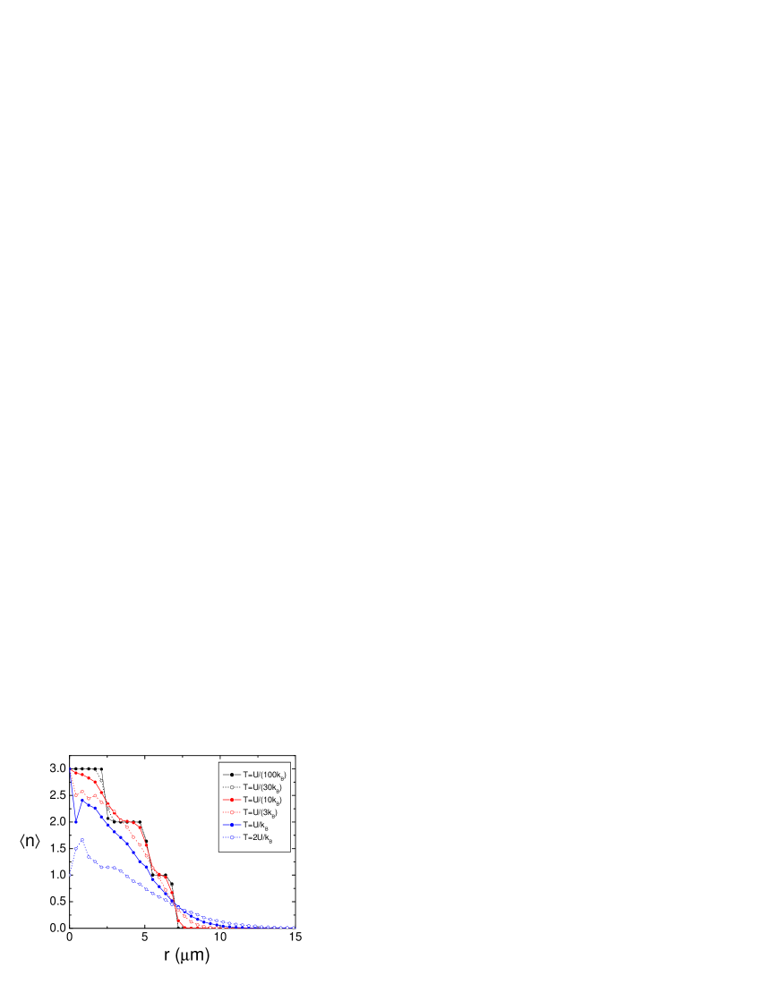
Figure 3: Spatial profile of occupation number for six different temperatures (see legend). A Metropolis algorithm is used to calculate the distribution of roughly $3\times 10^{4}$ atoms among lattice sites with a harmonic external potential characterized by $\alpha=h\times 113$ Hz$/\mu m^{2}$ and the experimental parameters detailed in the introduction. The average number of atoms per site $\langle n\rangle$ is shown at radii $r$ which are multiples of the lattice spacing. The radius is measured from the minimum of the external potential.

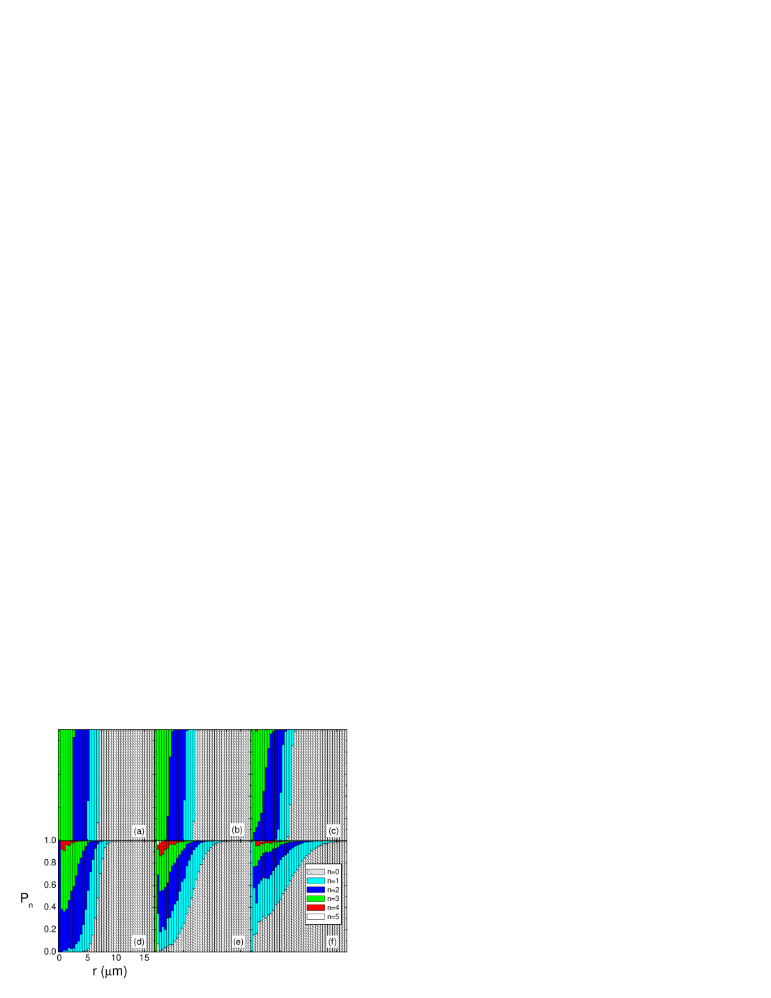
Figure 4: Probability distribution of occupation number for six different temperatures: (a) $U/(100k_{B})$, (b) $U/(30k_{B}$), (c) $U/(10k_{B}$), (d) $U/(3k_{B})$, (e) $U/k_{B}$, and (f) $2U/k_{B}$. The probability $P_{n}$ to find a site occupied by $n$ atoms is shown for radii $r$ which are multiples of the lattice spacing. The data are extracted from the Metropolis algorithm used in Fig. 3 and are displayed as a stacked column plot (see legend).

The time scale for thermally activated hopping can be probed in experiments and will play a role in schemes where a zero entropy state is initialized for neutral atom quantum computing Vala03 . At the crudest level of approximation, the tunneling rates due to quantum and thermal effects can be added to obtain the net rate, particularly if the time scales are widely separated HanggiTalknerBorkovec90 . At zero temperature we found that dynamic fluctuations of p-h excitations and site-defect propagation across potential barriers are largely suppressed due to interactions. However, at finite temperature, these processes can be thermally activated. To describe hopping between sites, one can invoke a phenomenological double well model and appeal to the exhaustive knowledge of reaction-rate theories for hopping between metastable states HanggiTalknerBorkovec90 .

IV Microwave Spectroscopy

In this section we describe a technique for probing the spatial structure and energy spectrum of the Mott-insulator state discussed in section II. The method, an extension of work in Rabl03 , is compatible with any lattice geometry and is capable of resolving the effects of finite temperature. In contrast to the previous sections of this paper where only one atomic internal state was considered, multiple hyperfine states are employed in our spectroscopic technique. Transitions between hyperfine states are driven using a microwave-frequency magnetic field. Information on the interaction energy $U$ and the density profile of the gas is obtained by manipulating the resonant transition frequency between hyperfine states. Dependence on site occupancy is achieved by changing the interaction energy $U$ using a Feshbach resonance, while a spatially inhomogeneous, state-dependent optical potential provides spatial resolution.

IV.1 Interaction with an oscillating magnetic field

We first address the atomic interaction with an oscillating magnetic field in anticipation of explaining the detailed experimental procedure in subsequent sections. In the presence of an oscillating magnetic field, the exact Hamiltonian at one lattice site in the absence of tunneling is

$$\left\{\hat{H}_{ab}\right\}+\hat{H}_{I} = \left\{\frac{U_{bb}}{2}\hat{n}_{b}(\hat{n}_{b}-1)+\right.$$ (33)

$$\left.\frac{U_{aa}}{2}\hat{n}_{a}(\hat{n}_{a}-1)+U_{ab}\hat{n}_{a}\hat{n}_{b}+\hbar\omega_{ab}\hat{n}_{b}\right\}$$

$$-\sum_{i}\hat{\vec{\mu}}^{(i)}\cdot\vec{B}$$

where $\hat{n}_{a}$ and $\hat{n}_{b}$ are the number operators for atoms in hyperfine states $|a\rangle$ and $|b\rangle$, $U_{aa}$, $U_{bb}$, and $U_{ab}$ are the interaction energy for two atoms in states $|a\rangle$ or $|b\rangle$ or one atom in each state, the sum runs over the atoms, and $\hat{\vec{\mu}}$ is the atomic magnetic moment operator. The energy difference $\hbar\omega_{ab}$ between states $|a\rangle$ and $|b\rangle$ takes into account the effect of any external optical and magnetic potentials, including a static magnetic bias field that defines the $z$ direction. We also assume that the lattice potential is identical for both hyperfine states; specifically we consider a far off-resonance lattice. The applied microwave-frequency magnetic field $\vec{B}=B_{l}\cos\left[\omega(t)t\right]\hat{e}_{x}$ may have a time-dependent frequency $\omega$. The interaction with the magnetic field (the last term in Eq. (33)) can be rewritten as $\hat{H}_{I}=\hbar\Omega[e^{i\omega(t)t}+e^{-i\omega(t)t}]\sum_{i}(\hat{\sigma}_{+}^{(i)}+\hat{\sigma}_{-}^{(i)})$ where $\hbar\Omega=-\mu_{ab}B_{l}/4$, $\mu_{ab}$ is the magnetic moment matrix element between the $|a\rangle$ and $|b\rangle$ states, and $\hat{\sigma}_{\pm}^{(i)}$ are the Pauli raising and lowering operators for atom $i$.

Because the states $|a\rangle$ and $|b\rangle$ form an effective spin-1/2 system, the eigenstates of $\hat{H}_{ab}$ are eigenstates of total angular momentum $\hat{J}=\sum_{i=1}^{n}\hat{S}^{(i)}$, where $\hat{S}^{(i)}$ is the effective spin operator for atom $i$. The interaction with the oscillating magnetic field, which can be rewritten as $\hat{H}_{I}=\Omega[e^{i\omega(t)t}+e^{-i\omega(t)t}](\hat{J}_{+}+\hat{J}_{-})$, causes a rotation of the total spin vector. Since we assume that all of the atoms start in one hyperfine state, $\hat{H}_{I}$ couples states with different $m_{j}$, but fixed total angular momentum quantum number $j=n/2$ ($n=n_{a}+n_{b}$ and $J^{2}|j,m_{j}\rangle=\hbar^{2}j(j+1)|j,m_{j}\rangle$). All states with $j=n/2$ are properly symmetrized with respect to two-particle exchange for bosons.

We take advantage of the Schwinger representation and write the eigenstates $|j,m_{j}\rangle$, which are states of $n$ spin-1/2 particles, as $|n_{a},n_{b}\rangle$. In this representation, $\hat{J}_{+}|n_{a},n_{b}\rangle=\sqrt{n_{a}(n_{b}+1)}|n_{a}-1,n_{b}+1\rangle$ and $\hat{J}_{-}|n_{a},n_{b}\rangle=\sqrt{n_{b}(n_{a}+1)}|n_{a}+1,n_{b}-1\rangle$.

The interaction picture is convenient for calculating the effect of the oscillating field. Taking into account that the interaction Hamiltonian can only couple states where $n_{a}$ changes by one, that $n_{a}+n_{b}$ is constant, and by making the rotating-wave approximation, we obtain

$$\hat{H}_{I}^{\prime} = \hbar\Omega\left\{\hat{J}_{+}e^{-i[\omega(t)-(E_{n_{a}-1,n_{b}+1}-E_{n_{a},n_{b}})/\hbar]t}+\right.$$ (34)

$$\left.\hat{J}_{-}e^{i[\omega(t)-(E_{n_{a},n_{b}}-E_{n_{a}+1,n_{b}-1})/\hbar]t}\right\}$$

in the interaction picture. In Eq. 34, the energy $E_{n_{a},n_{b}}|n_{a},n_{b}\rangle=\hat{H}_{ab}|n_{a},n_{b}\rangle$ is determined by the eigenvalues of $\hat{H}_{ab}$. The quantum state of the atoms on a lattice site can be written in terms of the time-independent eigenvectors of $\hat{H}_{ab}$ as

$$\Psi=\sum_{n_{a}=0}^{n}C_{n_{a},n_{b}=n-n_{a}}|n_{a},n_{b}=n-n_{a}\rangle$$ (35)

where $n=n_{a}+n_{b}$. In general, the Schrödinger equation gives rise to coupled equations for the $C_{n_{a},n_{b}}$ that can be solved numerically.

To illustrate the salient features of this interaction Hamiltonian, we will ignore off-resonant excitation and discuss the case $\omega(t)=E_{n_{a}-1,n_{b}+1}-E_{n_{a},n_{b}}+\delta(t)$. While for ⁸⁷Rb the interaction energy matrix elements are normally hyperfine-state-independent to within a few percent, we consider using a Feshbach resonance so that we can have $U_{ab}=U_{aa}$ and $U_{bb}=\beta U_{aa}$. We discuss only the states $n=0,1,2,3$ even though the proposed experimental techniques will work for any site occupancy. For typical experimental conditions, three-body recombination rates will limit the lifetime of the $n>2$ state to a few ms. However, we include analysis of that state here in light of a recent proposal Meystre2004 for reducing three-body recombination rates by a factor of 100.

The energy spectrum of the eigenstates of $\hat{H}_{ab}$ for states with different $n$ is shown in Fig. 5(a). Solving the Schrödinger equation for the atomic wavefunction gives coupled equations of the form

$$\dot{C}_{n_{a},n_{b}}=-i\Omega_{n_{a},n_{b}}C_{n_{a}+1,n_{b}-1}e^{-i\delta(t)}$$ (36)

$$\dot{C}_{n_{a}+1,n_{b}-1}=-i\Omega_{n_{a},n_{b}}C_{n_{a},n_{b}}e^{i\delta(t)}$$ (37)

where $\Omega_{n_{a},n_{b}}=\sqrt{(n_{a}+1)n_{b}}\Omega$. In the absence of off-resonant excitation and for $\delta$ independent of time, the problem reduces to oscillations between two states with Rabi frequency $\Omega_{n_{a},n_{b}}$ (shown in Fig. 5(b)). There are two important features of the coupled problem that are apparent in Fig. 5. The first is that there are no degenerate energy splittings in any manifold for constant $n$. However, the transition frequencies are degenerate when the transition involves states with the same $n_{b}$ between manifolds of different $n$. Also, the Rabi rates for transitions $|0,n\rangle\leftrightarrow|1,n-1\rangle$ and $|n,0\rangle\leftrightarrow|n-1,1\rangle$ are unique to each manifold of constant $n$, regardless of the value of $\beta$ (i.e., $|1,1\rangle\leftrightarrow|0,2\rangle$ and $|2,1\rangle\leftrightarrow|1,2\rangle$). In the next section, we will describe two experiments that will take advantage of these features.

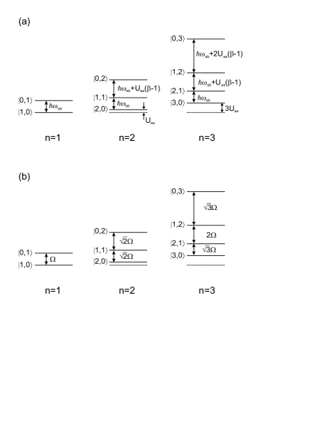
Figure 5: The energy spectrum of $\hat{H}_{ab}$ for lattice sites with $n=1,2,3$ (a) and the Rabi frequencies for transitions between states that are coupled by the interaction Hamiltonian (b). In (a), the energy difference between states and the shift of the ground state are shown.

IV.2 Experimental Proposals

The two experimental techniques that we describe in this section are a simple method for determining the ratios of sites with different $n$, and a more developed technique for mapping out the spatial structure of the insulator state. We consider experiments using ⁸⁷Rb atoms and the experimental parameters outlined in the introduction. With the laser intensity required to reach 30 $E_{R}$ lattice depths, spontaneous emission rates driven by the lattice light will be negligible on experimental timescales. The limiting timescale for experiments will therefore be collisions with residual gas molecules in the vacuum system or spontaneous scattering from an additional optical potential.

IV.2.1 Rabi oscillations

The first experiment that we propose uses Rabi oscillations as a probe of the total population in the lattice of sites with any $n$. A similar technique has been used in ion-trap experiments to measure populations in different harmonic oscillator levels Leibfried97a ; Meekhof96a ; BenKish2003 . The total number of sites with $n$ atoms is identified by the Rabi oscillation amplitude at the Rabi rate $\Omega_{n,0}$ for the $|n,0\rangle\leftrightarrow|n-1,1\rangle$ transition. Because the resonant frequency and Rabi oscillation rate for this transition are independent of interaction energy, this method is insensitive to the motional state of the atoms.

The gas is first prepared in the Mott-insulator state in the lattice; harmonic confinement is provided by an inhomogeneous magnetic field. The atoms in the lattice are initialized in the state $|a\rangle$ (through optical pumping, for example). A magnetic field at frequency $\omega_{ab}$ is applied to couple the $|a\rangle$ and $|b\rangle$ states, and the population in $|b\rangle$ is measured for different lengths of time of the applied coupling (via resonance fluorescence, for example). The data are fitted to a sum of oscillating functions with frequencies that differ by a factor $\sqrt{k}$ where $k=1,2,3...$. The total population in the lattice in states of different $n$ are then directly connected to the amplitudes of each oscillating term in the fit.

One complication with this scheme is that the inhomogeneous magnetic field will introduce a spread in $\omega_{ab}$ across the lattice, which will cause dephasing of the Rabi oscillations at different sites. To suppress shifts in $\omega_{ab}$ across the lattice, the energy difference between states $|a\rangle$ and $|b\rangle$ should be insensitive to magnetic field. This can be accomplished using a first-order magnetic field insensitive transition, for example between the states $|F=2,m_{F}=1\rangle$ and $|F=1,m_{F}=-1\rangle$ near 3.24 G Hall98a . For $10^{6}$ atoms, to realize sites with $n=3$ will require at least a 7 mG spread across the gas using either of these states. With a 3.24 G magnetic bias field, there will be less than a $2\pi\times 0.1$ Hz shift in $\omega_{ab}$ across the occupied sites.

IV.2.2 Rapid Adiabatic Passage

In this section, we explain an experimental technique to probe the Mott-insulator spatial structure directly, where the occupation of sites is identified using the interaction energy. Rapid adiabatic passage is used to transfer atoms in state $|a\rangle$ to state $|b\rangle$. The interaction energy is manipulated by using a Feshbach resonance such that the resonant microwave frequency shifts for transitions between $|a\rangle$ and $|b\rangle$ in a manifold of states with constant $n$. The maximum frequency shift dependence on $n$ permits unique identification of sites with different $n$.

To change the interactions between atoms in state $|b\rangle$, we choose $|b\rangle=|F=1,m_{F}=1\rangle$ and apply a uniform magnetic field with magnitude close to the ⁸⁷Rb Feshbach resonance at 1000.7 G Volz03 ; Marte02 . The magnitude of the field is adjusted so that $\beta=5$ ($U_{bb}=5U_{aa}$). Because this particular Feshbach is exceptionally narrow, applying a uniform magnetic field is necessary to avoid spatially-varying interaction energy shifts. Therefore, rather than obtaining spatial information by employing an inhomogeneous magnetic field, a spatially inhomogeneous near-resonant optical potential is used to shift $\omega_{ab}$. The near-resonant laser fields are engineered to provide a harmonic external potential; this may be accomplished using diffractive optics Curtis02 ; Sinclair04 to produce a focused laser beam with a parabolic intensity profile in three dimensions. To maximize the shift in $\omega_{ab}$ while minimizing spontaneous emission rates, we choose $|a\rangle$=$|F=2,m_{F}=2\rangle$ and tune the laser wavelength and polarization so that the optical potential for the $|b\rangle$ state vanishes. For different atoms, such as ⁸⁵Rb, with broader Feshbach resonances, the complication of employing an optical potential may not be necessary.

The overall effect of the applied, parabolic optical potential is to shift $\omega_{ab}=\omega_{0}-\gamma r^{2}$ parabolically in space. The curvature $\gamma$ is related to the curvature of the intensity profile of the near-resonant optical field, $\omega_{0}\approx 9.126$ GHz is determined by the atomic hyperfine structure and the magnetic bias field, and $r$ is the distance from the minimum of the parabolic optical potential. The spectrum for transitions between states $|a\rangle$ and $|b\rangle$ for sites with $n=1,2,3$ is shown in Fig. 6. For our experimental procedure, the curvature $\gamma$ is adjusted so that the minimum interaction energy shift is at least equal to the shift from the parabolic optical potential for the $n=2$ state at the boundary with the $n=1$ state. While this may be incompatible with supporting the desired Mott-insulator structure, the applied state-dependent potential can be switched quickly before the spectroscopy described next is performed.

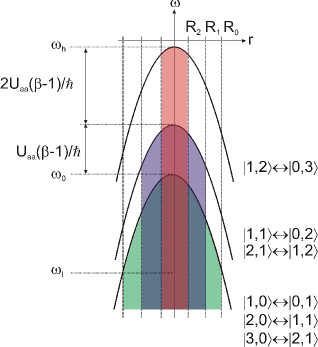
Figure 6: The spectrum for transitions between $|a\rangle$ and $|b\rangle$ for $n=1,2,3$. The transition frequency between states with different $n_{a}$ and $n_{b}$ is shown by the thick line. The dashed lines indicate the boundaries between sites with different $n$ in the lattice, which occur at radii $R_{0}$, $R_{1}$, and $R_{2}$. Sites with $n=1,2,3$ are indicated with green, blue, and red coloring, respectively. The interaction energy shifts are indicated, and the figure is drawn assuming $\beta>0$.

The experiment is performed by first preparing the atoms in the $|a\rangle$ state. Storing the atoms for long times in the $|b\rangle$ state while the magnetic field is near the Feshbach resonance is avoided to minimize effects due to inelastic collisions. A microwave frequency magnetic field is then swept from $\omega_{l}$ to $\omega_{h}$ and the number of atoms transferred to $|b\rangle$ is measured (using resonance fluorescence, for example) as the frequency is changed.

Atoms are transferred to state $|b\rangle$ in stages. As the frequency is swept toward $\omega_{h}$, one atom at all occupied sites is transferred to $|b\rangle$. This process is interrupted at $\omega_{0}$ by a gap where no atoms are transferred to $|b\rangle$ as the frequency is changed. The size of that gap in frequency $U_{aa}(\beta-1)/\hbar-\gamma R_{1}^{2}$ is related to the interaction energy, the size of the region where there are at least two atoms per site, and the curvature $\gamma$ of the optical potential. After this gap in atom transfer, one additional atom per site is transferred to state $|b\rangle$ for all sites that have at least two atoms per site. Another gap is encountered at $\omega_{0}+U_{aa}(\beta-1)/\hbar$ where no atoms are transferred that is $2U_{aa}(\beta-1)/\hbar-\gamma R_{2}^{2}$ wide in frequency. Finally, a third atom is transferred to $|b\rangle$ in each site where $n=3$ as the frequency is swept to $\omega_{h}$. No atoms are transferred to $|b\rangle$ as the frequency is increased past $\omega_{0}+3U_{aa}(\beta-1)/\hbar$. The interaction energy and the distribution of sites in space width different occupancy $n$ can be inferred from the number of atoms transferred to $|b\rangle$ as the frequency is changed.

This sequence of transfer between hyperfine states separated by gaps is generic to any Mott-insulator structure. Transfer begins at $\omega_{rf}=\omega_{0}-\gamma R_{0}^{2}$, which corresponds to the boundary of the occupied sites at $R_{0}$. The width of each gap where atoms are not transferred to $|b\rangle$ as the frequency is changed is $kU_{aa}(\beta-1)/\hbar-\gamma R_{k}^{2}$, where $k=1,2,3...$. The highest frequency where atoms is transferred is determined by the occupancy $m$ at the core and is $\omega_{0}+mU_{aa}(\beta-1)/\hbar$.

The results of a simulation of this experimental technique is shown in Fig. 7 for a gas consisting of roughly $3\times 10^{4}$ atoms at six different temperatures. The Metropolis algorithm is used to prepare the initial distribution of atoms among lattice sites at each finite temperature. An additional harmonic potential characterized by $\alpha=h\times 113$ Hz$/\mu m^{2}$ is applied to generate a Mott-insulator state with a core of $n=3$ sites at zero temperature. This same curvature $\gamma=113\times 2\pi$ Hz$/\mu m^{2}$ is used for the state-dependent optical potential while the oscillating magnetic field is applied. The Schrödinger equation is numerically solved on each lattice site using $\Omega=100\times 2\pi$ Hz and $\omega_{rf}(t)=6.4\times 10^{4}\times 2\pi\cdot t$ Hz. We would like to have spectral discrimination between sites at different radii, which limits the Rabi frequency $\Omega$ since it sets the effective bandwidth for transfer between states. Therefore we chose $\Omega$ so that it is comparable to the difference in $\omega_{ab}$ between sites spaced radially by $a$ near the minimum of the optical potential. The sweep rate for $\Omega$ is chosen so that Landau-Zener transitions are made with high probability. The data in Fig. 7 would be generated using a frequency sweep lasting $\sim 1.26$ seconds, which should be comparable with spontaneous scattering times and much faster than loss caused by collisions with residual background gas molecules.

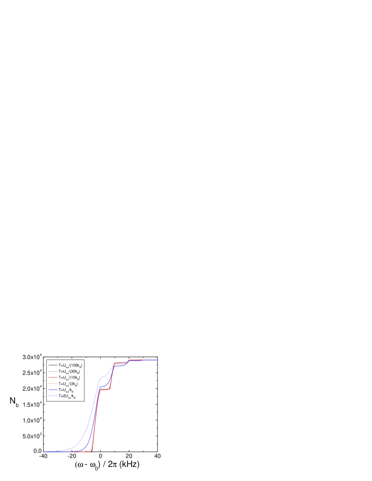
Figure 7: Simulation of rapid adiabatic passage experiment for roughly $3\times 10^{4}$ atoms at six different temperatures (see the legend, where $k_{b}$ is Boltzmann’s constant). The number of atoms $N_{b}$ in state $|b\rangle$ is shown as the frequency $\omega_{rf}$ of an oscillating magnetic field is swept.

From the simulation results shown in Fig. 7, it is clear that the effects of a state-dependent interaction persist to relatively high temperature compared with the interaction energy. The smallest frequency at which atoms are transferred to $|b\rangle$ decreases with increasing temperature as the size of the gas in the harmonic potential grows. In principle, the temperature of the gas can be inferred from a fit of data obtained using this technique to the simulation results.

V Concluding remarks

The possibility of exploring novel quantum phases of matter using ultra-cold atoms trapped in optical lattices has piqued the interest of many researchers. In this paper, we have detailed the necessary conditions for creating and probing a shell structure of Mott-insulator phases in an optical lattice. Instability of the Mott-insulator shell structure arises principally from two effects: finite tunneling and finite temperature. Finite tunneling of the bosons between neighboring sites leads to superfluid regions between the shells and particle-hole defects in the Mott-insulator regions. We have shown that for reasonable experimental parameters, these effects can be made negligible. The relevant conditions are both that the tunneling parameter must be small compared with the on-site repulsion ($w/U\ll 1$) and small compared with the typical change in the confining potential $V$ between neighboring sites ($w/\Delta V\ll 1$) across the Mott-insulator boundary. At finite temperature, while the Mott state formally ceases to exist, we have found a reasonable suppression of defects for temperatures lower than $U/(10k_{b})$ from Monte Carlo simulations of $3\times 10^{4}$ atoms. The existing literature on quantum tunneling at finite temperature provides a starting point for a more detailed exploration of these issues in this rich system, for instance, the effects of the coupling between a single site defect and the rest of the system. In this paper we have also proposed an experimental probe that has the capacity to spatially resolve the Mott-insulator shell structure.

B. DeMarco acknowledges support from the U.S. Office of Naval Research, award N000140410490. C. Lannert and S. Vishveshwara thank the KITP, where this work was initiated, for its hospitality and for valuable discussions. The authors would also like to thank A.J. Leggett for fruitful discussions.

References

- (1) D. Jaksch, C. Bruder, J.I. Cirac, C.W. Gardiner and P. Zoller, Phys. Rev. Lett. 81, 3108 (1998).
- (2) A. Kuklov, N. Prokof’ev, and B. Svistunov, Phys. Rev. Lett. 92, 050402 (2004).
- (3) E. Jane, G. Vidal, W. Dur, P. Zoller and J.I. Cirac, Quant. Inf. Comp. 3, 15 (2003).
- (4) D. van Oosten, P. vn der Straten, and H.T.C. Stoof, Phys. Rev. A 63, 053601 (2001).
- (5) V.A. Kashurnikov, N.V. Prokof’ev, and B.V. Svistunov, Phys. Rev. A 66, 031601(R) (2002).
- (6) G.G. Batrouni, V. Rousseau, R.T. Scalettar, M. Rigol, A. Muramatsu, P.J.H. Denteneer, and M. Troyer, Phys. Rev. Lett. 89, 117203 (2002).
- (7) S. Wessel, F. Alet, S. Trebst, D. Leumann, M. Troyer, and G. Batrouni, cond-mat/0411473 (2004).
- (8) P. Rabl, A.J. Daley, P.O. Fedichev, J.I. Cirac and P. Zoller, Phys. Rev. Lett. 91, 110403 (2003).
- (9) G.K. Brennen, G. Pupillo, A.M. Rey, C.W. Clark and C.J. Williams, quant-ph/0312069 (2003).
- (10) A. J. Leggett, S. Chakravarty, A. T. Dorsey, M. P. A. Fisher, A. Garg, and W. Zwerger Rev. Mod. Phys. 59, 1 (1987).
- (11) J. P. Sethna, Phys. Rev. B 24, 698 (1981); J. P. Sethna, ibid. 25, 5050 (1982); C. P. Flynn and A. M. Stoneham, ibid., 1, 3966, (1970); H. Teichler and A. Seeger, Phys. Lett. A 82, 91 (1981).
- (12) P. Hänggi, P. Talkner, and M. Borkovec, Rev. Mod. Phys. 62, 251 (1990).
- (13) T. Rom, T. Best, O. Mandel, A. Widera, Ma. Greiner, T.W. Hänsch, and I. Bloch, Phys. Rev. Lett. 93, 073002 (2004).
- (14) J. Vala, A.V. Thapliyal, S. Myrgren, U. Vazirani, D.S. Weiss and K.B. Whaley, quant-ph/0307085 (2003).
- (15) M. Greiner, O. Mandel, T. Esslinger, T.W. Hansch and I. Bloch, Nature 415, 39 (2002).
- (16) M. P. A. Fisher, P. B. Weichman, G. Grinstein, and D. S. Fisher, Phys. Rev. B 40, 546 (1989).
- (17) M. Greiner, Ph.D. Dissertation, Ludwig-Maximilians-Universität at München (2003).
- (18) S. Sachdev, Quantum phase transitions (Cambridge University Press, 1999).
- (19) M. Nielsen and I. Chuang, Quantum Computation and Quantum Information (Cambridge Univ. Press, 2000).
- (20) D.B.M. Dickerscheid, D.van Oosten, P.J.H. Denteneer, and H.T.C. Stoof, Phys. Rev. A 68, 043623 (2003).
- (21) C.P. Search, W. Zhang, and P. Meystre, Phys. Rev. Lett. 92, 140401 (2004).
- (22) A. Ben-Kish, B. DeMarco, V. Meyer, M. Rowe, J. Britton, W.M. Itano, B.M. Jelenkovic, C. Langer, D. Leibfried, T. Rosenband and D.J. Wineland, Phys. Rev. Lett. 90, 037902 (2003).
- (23) D. Leibfried, D.M. Meekhof, C. Monroe, B.E. King, W.M. Itano and D.J. Wineland, J. Mod. Opt. 44, 2485 (1997).
- (24) D.M. Meekhof, C. Monroe, B.E. King, W.M. Itano and D.J. Wineland, Phys. Rev. Lett. 76, 1796 (1996).
- (25) D.S. Hall, M.R. Matthews, C.E. Wieman and E.A. Cornell, Phys. Rev. Lett. 81, 4532 (1998).
- (26) T. Volz, S. Durr, S. Ernst, A. Marte and G. Rempe, Phys. Rev. A 68, 010702(R) (2003).
- (27) Marte, T. Volz, J. Schuster, S. Durr, G. Rempe, E.G.M. van Kempen and B.J. Verhaar, Phys. Rev. Lett. 89, 283202 (2002).
- (28) J.E. Curtis, B.A. Koss and D.G. Grier, Opt. Comm. 207, 169 (2002).
- (29) G. Sinclair, P. Jordan, J. Leach, M.J. Padgett, and J. Cooper, J. Mod. Opt. 51, 409 (2004).