One-dimensional itinerant ferromagnets with Heisenberg symmetry and the ferromagnetic quantum critical point

Abstract

We study one-dimensional itinerant ferromagnets with Heisenberg symmetry near a ferromagnetic quantum critical point. It is shown that the Berry phase term arises in the effective action of itinerant ferromagnets when the full SU(2) symmetry is present. We explicitly demonstrate that dynamical critical exponent of the theory with the Berry term is $z=2+{\rm O}(\epsilon^{2})$ in the sense of $\epsilon$ expansion, as previously discovered in the Ising limit. It appears, however, that the universality class at the interacting fixed point is not the same. We point out that even though the critical theory in the Ising limit can be obtained by the standard Hertz-Millis approach, the Heisenberg limit is expected to be different. We also calculate the exact electron Green functions $G(x,t=0)$ and $G(x=0,t)$ near the transition in a range of temperature, which can be used for experimental signatures of the associated critical points.

I Introduction

Quantum phase transitions from a paramagnetic to a ferromagnetic (FM) state in two and three dimensional itinerant electron system have been studied extensively in the past hertz ; andy1 . The standard approach in studying such systems, first advocated by Hertz hertz , involves two steps. First, one decouples the electron-electron interaction term in the Hamiltonian using a Hubbard-Stratonovitch transformation. Next, the fermions are integrated out to obtain an effective Landau-Ginzburg (LG) theory in terms of the FM order parameter which provides an effective description of the transition. However, it has been recently pointed out that the procedure of integrating out the gapless fermions in the above mentioned scheme might be tricky kirk . In particular, it might lead to singular terms in the effective LG functional which can change the critical property of the transition.

In contrast, very little attention has been paid to such transitions in one dimension (1D), partly due to the Lieb-Mattis theorem lm which states that the ground states of one-dimensional Hubbard models with nearest-neighbor hopping and density dependent short-range interaction are always spin singlets. However, numerical work carried out in Ref. daul, , has shown that the presence of a next-nearest-neighbor hopping term in the above mentioned class of models can result in a FM ground state. The properties of such ’FM Luttinger liquids’ has been studied in detail in Ref. lorenz, . Recently, a bosonization analysis has also been carried out to study the paramagnetic-FM transition in 1D Hubbard models with Ising symmetry yang1 . It is shown that in $d=1$, the critical theory is below its upper critical dimension and is governed by an interacting fixed point. A similar conclusion was reached in Ref. subir2, from analysis of rotor models of ferromagnets.

In this work, we carry out a similar analysis which applies for Heisenberg ferromagnets by explicitly keeping track of the full SU(2) symmetry of the model. In particular, we show that at the Gaussian level, the presence of a Berry phase term in the effective action of such ferromagnets does not change the dynamical critical exponent $z$ of the transition: $z=2+{\rm O}(\epsilon^{2})$ in the $\epsilon$ expansion sense. We point out that in spite of the same value of the dynamical critical exponent $z$ at the Gaussian level, the universality class of this transition can be different from its Ising counterpart. Our analysis also shows that contrary to the claim of Ref. yang1, , the critical theory for Ising symmetry can be obtained by the standard Hertz-Millis procedure and in 1D such a procedure is identical to the bosonization approach for Ising FM quantum critical points. However, for the SU(2) case, it appears that the critical theory may not be described by the standard Hertz-Millis procedure. We also consider the effect of the FM critical fluctuations on the electron Green function at finite temperature. We obtain an exact expression for the electron Green functions $G(x=0,t)$ and $G(x,t=0)$ in a temperature range, which can be accessed experimentally by measuring the tunneling density of states (DOS) and the momentum distribution function respectively.

The organization of the paper is as follows. In the next section, we obtain the effective action for 1D quantum ferromagnets with Heisenberg symmetry at the Gaussian level and determine $z$ by analyzing this action. Then we discuss the interacting fixed point in the $\epsilon$-expansion sense and the issue of universality of the Ising and Heisenberg cases in the light of possible quartic couplings. This is followed by Sec. III, where we obtain the electron Green’s function at finite temperature. We summarize and discuss our results in Sec. IV.

II Critical theory in the Heisenberg limit

We first derive the effective action for the critical theory by incorporating the transverse spin fluctuations in Sec. II.1. This is followed by the analysis of the effective action to derive the dynamical critical exponent $z$ in Sec. II.2.

II.1 Derivation of the effective action

We start from a one dimensional $t$-$J$ model given by

$${\mathcal{H}} = -\sum_{<ij>}\left[\sum_{\sigma}t\left(\psi_{i\sigma}^{\dagger}\psi_{j\sigma}+{\rm h.c.}\right)+J{\bf S}_{i}\cdot{\bf S}_{j}\right]$$ (1)

where $\psi_{i\sigma}$ represents an electron at site $i$ with spin $\sigma$, and ${\bf S}$ denotes the electron spin operators $S_{ia}=\psi_{i}^{\dagger}\sigma_{a}\psi_{i}$ where $\sigma_{a}$ are the usual Pauli matrices. The corresponding action can be written as

$$S = \int dx\int_{0}^{\beta}d\tau\left[\psi^{\dagger}(x,\tau)\left(\partial_{\tau}-\mu\right)\psi(x,\tau)+{\mathcal{H}}\right]$$ (2)

where $\tau$ is the imaginary time and $\beta=1/k_{B}T$ denotes inverse temperature. Note that $\psi^{\dagger}=(\psi^{\dagger}_{\uparrow},\psi^{\dagger}_{\downarrow})$ and $\psi=(\psi_{\uparrow},\psi_{\downarrow})^{T}$ are spinor representations of the electron operators. We have switched to a continuous representation of space and this amounts to replacing the last term in Eq. 1 by $-\int dxdx^{\prime}J(x-x^{\prime}){\bf S}(x)\cdot{\bf S}(x^{\prime})$ where $J(q)=J\cos(q_{x}a)$, where $a$ is the lattice spacing and we shall consider $J>0$ throughout as appropriate for studying a ferromagnetic instability.

Next, following Schultz schulz1 , we introduce new fermionic fields $\psi^{\prime}$ defined as $\psi(x,\tau)=U(x,\tau)\psi^{\prime}(x,\tau)$. Here $U$ represent SU(2) rotation matrices such that $U^{\dagger}(x,\tau){\bf\sigma}\cdot{\bf n}(x,\tau)U(x,\tau)=\sigma_{z}$. The unitary matrices $U$ therefore correspond to the rotations of the local spin quantization axis of the electrons to ${\hat{z}}$. The action $S$, in terms of these new fields, becomes

$$S = S_{0}+S_{J}$$

$$S_{0} = \int dxd\tau\ \psi^{\prime\dagger}\Big{[}\partial_{\tau}-\mu-C_{0}-2t\cos\left(-i\partial_{x}-C_{x}\right)\Big{]}\psi^{\prime}$$

$$S_{J} = -\int d\tau dxdx^{\prime}\ J(x-x^{\prime})S^{z}(x)S^{z}(x^{\prime})$$ (3)

where the fields $C_{\mu}=-iU^{\dagger}\partial_{\mu}U=\sum_{a=x,y,z}\sigma_{a}\Omega_{\mu}^{a}/2$ are the SU(2) gauge fields which describes the spin fluctuations of the system, $\mu=(\tau,x)$ refers to the time and space components of the fields and $\partial_{\mu}=(i\partial_{\tau},\partial_{x})$. The gauge freedom here consists of rotation of the spin of the $\psi^{\prime}$ fields about the $\hat{z}$ axis: $\psi^{\prime}\rightarrow\psi^{\prime}\exp\left(i\sigma_{z}\Phi\right)$. Such a rotation changes $\Omega_{\mu}^{z}\rightarrow\Omega_{\mu}^{z}+\partial_{\mu}\Phi$ and therefore leaves the action invariant.

From now on we shall replace $\psi^{\prime}$ by $\psi$ for notational convenience. The fermion fields can be written in terms of the right and the left movers: $\psi(x)=\psi_{L}(x)e^{-ik_{F}x}+\psi_{R}(x)e^{ik_{F}x}$, where $k_{F}$ is the Fermi wavevector. The right and the left moving fermions have energy dispersion

$$\epsilon_{\alpha}(k_{x}) = {\rm sgn}(\alpha)v_{F}k_{x}+\frac{k_{x}^{2}}{2m}$$ (4)

where $v_{F}=2ta\sin\left(k_{F}a\right)$ is the Fermi velocity and $m=1/\left[4ta^{2}\cos\left(k_{F}a\right)\right]$ is the mass for the fermions and ${\rm sgn}(\alpha)=+(-)$ for $\alpha=R(L)$. In most of our analysis, we shall restrict ourselves to the linearized dispersion relation for the fermions, which amounts to neglecting the quadratic term in $\epsilon_{\alpha}(k_{x})$. However, for deriving an effective action for the spin-fluctuations we shall need to retain the quadratic term, and hence it can not be neglected at the outset nicolas1 .

In terms of these fields, the action reads

$$S = S_{0}+S_{1}+S_{2}+S_{J}$$

$$S_{0} = \int d^{2}k\sum_{\alpha}\psi_{\alpha}^{\dagger}(k)G_{0}^{-1}\psi_{\alpha}(k)$$ (5)

$$S_{1} = \int d^{2}k\ d^{2}p\sum_{\alpha}\psi_{\alpha}^{\dagger}(k+p)$$ (6)

$$\times\left[\frac{\partial G_{0}^{-1}}{\partial k_{\mu}},C_{\mu}(p)\right]_{+}\psi_{\alpha}(k)$$

$$S_{2} = \int d^{2}k\ d^{2}p\sum_{\alpha}\psi_{\alpha}^{\dagger}(k+p)$$ (7)

$$\times\left[\frac{\partial^{2}G_{0}^{-1}}{\partial k_{\mu}^{2}},C_{\mu}^{2}(p)\right]_{+}\psi_{\alpha}(k)$$

$$S_{J} = -\int d^{2}q\sum_{\alpha\alpha^{\prime}}J_{\alpha\alpha^{\prime}}(q)S_{\alpha}^{z}(q)S_{\alpha^{\prime}}^{z}(-q)$$ (8)

Here $\int d^{2}k$ is the shorthand notation for $\beta^{-1}\sum_{\omega_{n}}\int dk_{x}/(2\pi)$, $k_{\mu}=(i\omega_{n},k_{x})$, $[..]_{+}$ denotes anticommutator, $\alpha$ denotes the $R,L$ indices for the right(R) and left(L) moving fermions, $G^{-1}_{0}=i\omega_{n}-\epsilon_{\alpha}(k_{x})$ is the free fermion propagator, and $J_{\alpha\alpha^{\prime}}(q)=J_{\alpha\alpha^{\prime}}\cos(q_{x})$. We have neglected all $2k_{F}$ terms in $S$ since we shall be primarily interested in studying the action near a ferromagnetic instability. The matrix $J_{\alpha\alpha^{\prime}}=J+\delta J\delta_{\alpha\alpha^{\prime}}$ has an additional $\delta J$ term in its diagonal components, which is added to make the matrix $J$ invertible and will be set to zero at the end of the calculation. The term $S_{2}$ (7) represents the diamagnetic term of the SU(2) gauge fields $C_{\mu}$ and is known to be important for deriving a low energy effective description of the spin fluctuations. Note that to obtain this term, one needs to go retain the quadratic term in $\epsilon_{\alpha}(k_{x})$ nicolas1 .

We then carry out a Hubbard-Stratonovitch transformation to decouple $S_{J}$:

$$S = S_{0}+S_{1}+S_{2}+S_{I}+S_{\phi}$$

$$S_{I} = \int d^{2}k\sum_{\alpha}i\phi_{\alpha}(k)S^{z}_{\alpha}(-k)$$ (9)

$$S_{\phi} = -\frac{1}{4}\int d^{2}k\sum_{\alpha\alpha^{\prime}}(J(q))^{-1}_{\alpha\alpha^{\prime}}\phi_{\alpha}(q)\phi_{\alpha^{\prime}}(-q)$$ (10)

Notice that the field $\phi$ does not correspond to the physical spin-density fields, but their conjugate. However, for studying the ferromagnetic instability, it is preferable to look at the physical spin-density fields. We therefore introduce these fields $\rho$ via a second Hubbard-Stratonovitch transformation which decouples $S_{\phi}$:

$$S = S_{0}+S_{1}+S_{2}+S_{\rm int}+S_{\rm HS}$$

$$S_{\rm int} = \int d^{2}k\sum_{\alpha}i\phi_{\alpha}(k)\left[S^{z}_{\alpha}(-k)-\rho_{\alpha}(-k)\right]$$ (11)

$$S_{\rm HS} = -\int d^{2}k\sum_{\alpha\alpha^{\prime}}J_{\alpha\alpha^{\prime}}(q)\rho_{\alpha}(q)\rho_{\alpha^{\prime}}(-q)$$ (12)

The next task is to integrate out the fermionic fields and obtain an effective low-energy description of the system in terms of the fields $C_{\mu}$, $\rho$ and $\phi$. This procedure turns out to be quite subtle as discussed in Ref. nicolas1, , but can be carried out comment1 . The resulting effective action, to Gaussian order, reads

$$S_{\rm eff} = S_{\rm NLSM}+S_{\rm Berry}+S[\rho,\phi]$$ (13)

$$S_{\rm NLSM} = \frac{N(0)}{4}\int d\tau dx\left[\left(\partial_{\tau}{\bf n}\right)^{2}+v_{F}^{2}\left(\partial_{x}{\bf n}\right)^{2}\right]$$ (14)

$$S_{\rm Berry} = \int d^{2}q\Omega_{0}^{z}(q)\sum_{\alpha}\rho_{\alpha}(-q)$$ (15)

$$S[\rho,\phi] = \int d^{2}q\sum_{\alpha\alpha^{\prime}}\Bigg{(}\frac{1}{2}\phi_{\alpha}\Pi_{\alpha\alpha^{\prime}}^{-1}\phi_{\alpha^{\prime}}-i\phi_{\alpha}(q)\rho_{\alpha^{\prime}}(-q)\delta_{\alpha\alpha^{\prime}}$$ (16)

$$-J_{\alpha\alpha^{\prime}}(q)\rho_{\alpha}(q)\rho_{\alpha^{\prime}}(-q)\Bigg{)}$$

where we have expressed $S_{\rm NLSM}$ in terms of the unit vector field ${\bf n}$ using the identity nicolas1 : ${\rm Tr}\left[C_{\mu}\right]^{2}-{\rm Tr}\left[\sigma_{z}C_{\mu}\right]^{2}=\left(\partial_{\mu}{\bf n}\right)^{2}/4$. The Berry phase term $S_{\rm Berry}$, as is well known, can not be expressed in terms of ${\bf n}$ vector since $\Omega_{0}^{z}$ depends on gauge choice of the SU(2) fields subir1 . The polarization tensor $\Pi_{\alpha\alpha^{\prime}}$ in $S[\rho,\phi]$ is given by

$$\Pi_{\alpha\alpha^{\prime}}^{-1}(q)=\delta_{\alpha\alpha^{\prime}}N(0)\frac{{\rm sgn}(\alpha)v_{F}q}{-iq_{0n}+{\rm sgn}(\alpha)v_{F}q}$$ (17)

Within the linearized dispersion and in one dimension Eq. 16 is known to be exact Kopietz .

We now introduce the spin-density fields in the symmetric(S) and the antisymmetric(A) channels $\rho_{S(A)}=\left(\rho_{R}+(-)\rho_{L}\right)$, integrate out the auxiliary fields $\phi_{\alpha}$ from Eq. 16. Since the ferromagnetic instability corresponds to the instability of the spin-density fields in the symmetric channel, we also integrate out the $\rho_{A}$ to obtain an effective action for $\rho_{S}$

$$S_{\rm eff} = S_{\rm NLSM}+S_{\rm Berry}+S[\rho_{S}]$$ (18)

$$S_{\rm Berry} = \int d^{2}q\Omega_{0}^{z}(q)\rho_{S}(-q)$$ (19)

$$S[\rho_{S}] = \int d^{2}q\rho_{S}(q){\mathcal{S}}_{S}(q)\rho_{S}(-q)$$

$$= -\int d^{2}q\rho_{S}(q)\left(\frac{q_{0}^{2}}{v_{F}^{2}q^{2}}-r-bq^{2}\right)\rho_{S}(-q)$$

where $r=(1-JN(0))$, $b=JN(0)a^{2}/2$, and $a$ is the lattice spacing. Here we have Wick-rotated back to real frequency and expanded $J(q)\simeq J(1-q_{x}^{2}a^{2}/2)$ . Notice that the ferromagnetic instability in Eq. LABEL:critical is signaled by $r=0$ or $JN(0)=1$ which agrees with the usual Stoner criteria for ferromagnets.

We would like to stress that, unlike the Ising case studied in Ref. yang1, , our final effective action (Eq. 18) is not only $S[\rho_{S}]$, but also contains $S_{\rm NLSM}$ and $S_{\rm Berry}$. This is crucial for a correct description of the transverse spin fluctuations which are natural consequence of the SU(2) symmetry of the problem. This point is best illustrated by studying the action (Eq. 18) inside the FM phase. Here the spin-density fields are gapped out and $\left<\rho_{S}\right>=M$, where $M$ is the magnetization of the system. In the FM phase, the low energy theory is therefore described by $S_{\rm NLSM}$ and $S_{\rm Berry}$. Note that the presence of the Berry phase term is crucial for the $k_{x}^{2}$ dispersion of the spin waves, as pointed out in Ref. wen, in the context of 2D ferromagnets. A similar analysis in this line for the Ising limit would yield Eq. LABEL:critical as the final effective action which is exactly the same result obtained in Ref. yang1, .

We also note that a similar procedure can be carried out in higher dimension. In that case, due to the presence of a continuous isotropic Fermi surface, instead of two Fermi points, the index $\alpha$ becomes the momentum $k_{\parallel}$ along the Fermi surface and the sum over $\alpha$ has to be replaced by an integral over $k_{\parallel}$. This changes the $q_{0}^{2}/(v_{F}^{2}q^{2})$ term in ${\mathcal{S}}_{S}(q)$ (Eq. LABEL:critical) to $|q_{0}|/(v_{f}q)$ and immediately leads to $z=3$. This result can also be alternatively obtained by finite dimensional bosonization technique Kopietz .

II.2 Analysis of the effective action and critical theory

We now analyze the critical theory for 1D. Our starting point is Eq. 18 derived in the previous subsection. From Eq. 14, the fluctuations of the ${\bf n}$ field are gapless in the Heisenberg limit, it is not a priori clear whether the coupling of $\rho_{S}$ to these fluctuations changes the universality class of the transition. To check this, we aim to integrate out the transverse fluctuation modes to obtain the final effective action in terms of the $\rho_{S}$ fields. To this end, we rewrite the action $S_{\rm NLSM}$ and $S_{\rm Berry}$ using the CP(1) representation. In this representation, the unit vector field ${\bf n}$ is represented by two complex fields $(z_{1},z_{2})$ with the constraint $|z_{1}|^{2}+|z_{2}|^{2}=1$. Following Refs. Witten, ; adda, , one can write

$$S_{\rm NLSM} = \int dt\ dx\sum_{j=1,2}|\left(\partial_{\mu}-iA_{\mu}\right)z_{j}|^{2}+\lambda(|z_{j}|^{2}-1)$$

where the U(1)gauge fields $A_{\mu}$ are given by

$$A_{\mu} = \Omega_{\mu}^{z}=i\sum_{j}\left[z_{j}^{\ast}\partial_{\mu}z_{j}-(\partial_{\mu}z_{j}^{\ast})z_{j}\right]$$ (22)

The field $\lambda$ is a Lagrange multiplier field used to implement the constraint of unit norm for the CP(1) fields. Note that in this representation, $S_{\rm Berry}$ can be written as

$$S_{\rm Berry} = \int d^{2}qA_{0}(q)\rho_{S}(-q)$$ (23)

and has the convenient interpretation of the action describing coupling of a U(1) scalar potential to matter field.

To describe the Berry term in a gauge invariant fashion, we now define a spin-current $j_{x}^{z}$ which satisfies the continuity relation

$$\partial_{t}\rho_{s}+\partial_{x}j_{x}^{z} = \partial_{\mu}J_{\mu}(x)=0$$ (24)

and write the Berry term as

$$S_{\rm Berry} = \int d^{2}qA_{\mu}(q)J_{\mu}(-q)$$ (25)

Although this procedure seems ad-hoc, the additional term in $S_{\rm Berry}$ introduced here could easily be obtained rigorously from our starting action (Eq. 3) if we carried out the analysis in the presence of a spin-current interaction term $H_{\rm current}=-\int dx\int dx^{\prime}\,K(x-x^{\prime}){\bf j}(x)\cdot{\bf j}(x^{\prime})$ where $j_{x}^{\alpha}=\psi^{\dagger}\sigma^{\alpha}\partial_{x}\psi(x)$ is the spin-current operator. Such a current-current interaction term, although always present in principle, is usually neglected since it is very small (O($v_{F}^{2}/c^{2}$)) compared to $S_{J}$. The only relevant information, apart from the continuity condition (24), that we shall need for our analysis here is that the spin-current correlator in the symmetric channel is given by comment2

$${\mathcal{K}}_{S}(q) = -v_{F}^{2}\left(\frac{q_{0}^{2}}{v_{F}^{2}q^{2}}-1+K\cos(qa)N(0)\right)$$

$$\simeq-v_{F}^{2}\left(\frac{q_{0}^{2}}{v_{F}^{2}q^{2}}-r^{\prime}\right)$$

where $r^{\prime}=1-KN(0)$. We therefore simply use this information and avoid carrying out a detailed analysis involving $H_{\rm current}$. Note that the propagator ${\mathcal{K}}_{S}$ is always massive near the critical point. Hence it is not necessary to retain the $q^{2}$ term in its expression.

At this stage, we find that to understand the effect of $S_{\rm Berry}$ on the ferromagnetic quantum critical point, we need to obtain an effective action for the gauge fields $A_{\mu}$. This involves integrating out the fields $z$ and $\lambda$ from $S_{\rm NLSM}$. It is well known that such an analysis can be reliably carried out for CP($N-1$) theories only in the large $N$ limit Witten ; adda . However, it is conjectured in Ref. Witten, that the qualitative results hold even for $N=2$. We therefore follow the large $N$ analysis of Refs. Witten, ; adda, to obtain

$$S_{\rm eff} = S_{\rm gauge}+S_{\rm Berry}+S_{\rm matter}$$ (27)

$$S_{\rm gauge} = -\int d^{2}pA_{\mu}(p)\left(p^{2}\delta_{\mu\nu}-p_{\mu}p_{\nu}\right)A_{\nu}(-p)$$ (28)

$$= \int d^{2}pA_{\mu}(p)G_{\mu\nu}^{\rm bare}(p)A_{\nu}(-p)$$

where $p_{\mu}=(p_{0},v_{F}p_{x})$. Notice that the propagator $G^{\rm bare}$ is not invertible. This problem can be easily taken care of by simply adding a gauge fixing term, as is customary for the photon propagator in QED. However, we shall not need to invert the bare propagator at any stage of our analysis, and hence retain the form of $G^{\rm bare}$ as given in Eq. 28. The action $S_{\rm matter}$ has now to be supplemented by a quadratic term in the spin current $j_{x}^{z}$ which involves

$$S_{\rm matter} = \int d^{2}q\Big{[}\rho_{S}(q){\mathcal{S}}_{S}(q)\rho_{S}(-q)$$ (29)

$$+j_{x}^{z}(q){\mathcal{K}}_{S}(q)j_{x}^{z}(-q)\Big{]}$$

The final step is to integrate out the gauge fields. To do this, we first integrate out the matter field $J_{\mu}$ and obtain an effective dressed propagator $G^{\rm dressed}$ for the gauge fields $A_{\mu}$

$$G^{\rm dressed}(k) = -\left(\begin{array}[]{cc}v_{F}^{2}k_{x}^{2}+\frac{1}{4{\mathcal{S}}_{S}(k)}&\omega v_{F}k_{x}\cr\omega v_{F}k_{x}&\omega^{2}+\frac{1}{4{\mathcal{K}}_{S}(k)}\end{array}\right)$$ (32)

We then replace $G^{\rm bare}$ by $G^{\rm dressed}$ in Eq. 28, and integrate out the gauge fields to obtain the contribution $\delta S$ of the gauge fields to the effective action for the matter fields $J_{\mu}$ comment3

$$S^{\prime}_{\rm eff} = S_{\rm matter}+\delta S$$

$$\delta S = \int d^{2}J_{\mu}(p)(\delta P)_{\mu\nu}(p)J_{\nu}(-p)$$ (34)

$$\delta P(k) = \frac{{\mathcal{K}}_{S}(k){\mathcal{S}}_{S}(k)}{{\mathcal{K}}_{S}(k)\omega^{2}+v_{F}^{2}k_{x}^{2}{\mathcal{S}}_{S}(k)^{2}+1/4}$$ (37)

$$\times\left(\begin{array}[]{cc}\omega^{2}+\frac{1}{4{\mathcal{K}}(k)}&-\omega v_{F}k_{x}\cr-\omega v_{F}k_{x}&v_{F}^{2}k_{x}^{2}+\frac{1}{4{\mathcal{S}}_{S}(k)}\end{array}\right)$$

Note that the term $\delta S$ couples the $\rho_{S}$ and $j_{x}^{z}$ fields. To obtain the effective action for the $\rho_{S}$ fields, we integrate out the $j_{x}^{z}$ fields and evaluate the resulting propagator at the critical point $r=0$ and retain the lowest order terms in $\omega$ and $k$. After some straightforward algebra, one obtains the correction term $\delta S^{\prime}[\rho_{S}]$

$$\delta S^{\prime}[\rho_{S}]\simeq-\int d^{2}k\rho_{S}(k)\left(\frac{\omega^{2}}{v_{F}^{2}k_{x}^{2}}-k_{x}^{2}+...\right)\rho_{S}(-k)$$ (38)

where the ellipsis represent terms which are higher order in $\omega$ and $k_{x}$. So we conclude that the effect of the Berry term is merely to renormalize the coefficients of the existing terms in $S[\rho_{S}]$. The critical theory obtained by integrating out the transverse fluctuation at the Gaussian level thus has $z=2$. By the usual $\epsilon$ expansion argument, we expect this analysis to give correct value of $z$ to ${\rm O}(\epsilon^{2})$.

Next we comment on the universality class of the transition. To determine the universality class, since we are below the upper critical dimension of the theory, we need to retain the possible fourth order diagrams while integrating out fermions in Eq. II.1. Two such representative diagrams are shown in Fig. 1. The diagram in the left panel is present for the Ising ferromagnets studied in Ref. yang1, , while that in the right panel is a consequence of the Heisenberg symmetry of the problem. After some algebra Kopietz , one can show that the diagram in the left panel of Fig. 1 generates Ising type contributions $\sim\int dxdt\rho_{S}^{4}$ while the diagram in the right panel generates, for example, quartic couplings $\sim\int dxdt\rho_{S}^{2}(\partial_{x}{\bf n})^{2}$ (apart from other similar quartic and higher order terms). The former type of terms are exactly those that are expected at quartic order for the Ising ferromagnets, either from a bosonization analysis yang1 or Hertz-Millis approach hertz ; andy1 . Therefore, our analysis shows that the standard Hertz-Millis procedure in 1D, gives exactly the same critical theory as obtained in Ref. yang1, by bosonization for the Ising case.

Figure 1: Representative diagrams for quartic coupling terms for Heisenberg theory. The left diagram is also present for Ising ferromagnets and generates the usual $\rho_{S}^{4}$ interaction term. The diagram on the right side generates quartic couplings between $\rho_{S}$ and ${\bf n}$ fields (see discussion in text), and has no analog in Ising ferromagnets. The internal lines involve Fermion Green functions and the vertices represent either $\sigma_{z}$ or $\Lambda^{\mu}_{a}=\sigma_{a}\partial G_{0}^{-1}/\partial k_{\mu}$ as shown. Both the diagrams are nonzero only if the Fermion dispersion has a non-zero curvature.

The latter type of diagrams are absent in the Ising model studied in Ref. yang1, . In the FM phases, where the amplitude mode is gapped, these terms represents a trivial renormalization of the parameters such as spin-wave stiffness of $S_{\rm NLSM}$ (Eq. 14). Near the transition, they generate quartic coupling between the amplitude and the spin-wave modes. Notice that these terms are different from the standard ${\bf m}^{4}$ quartic terms expected from the usual Hertz-Millis analysis of a Heisenberg magnet with a vector order parameter. We expect such quartic coupling terms to change the universality class of the transition from that of Ising ferromagnets. A determination of the universality class would therefore require a detailed analysis of Eq. 18 supplemented with all such possible relevant quartic coupling terms. In particular, this requires a consideration of both coupled longitudinal and transverse modes at the same footing. In this work, we shall be content with pointing out the necessity of such an analysis.

The quartic terms mentioned above makes the Gaussian fixed point, described by Eq. 18, unstable. However, all such diagrams, including the Ising type quartic terms, are non-zero only when the fermionic dispersion has a finite curvature yang1 ; Kopietz . Thus, above a temperature scale set by this curvature, the properties of the system is expected to be well described by the Gaussian theory described by Eq. 18. We discuss this point in more details in the next section.

III Electron Green’s function

It is well known that the presence of a quantum critical point shows up in experimentally accessible quantities such as tunneling DOS and the momentum distribution function of the electrons. To obtain these quantities one needs to estimate the effect of critical fluctuations on the electron Green function. However, the fixed point concerned here is an interacting one. This means to compute the electron Green function at $T=0$ near the critical point, one needs to solve the problem of electrons coupled to $interacting$ bosons. For the Ising ferromagnets these bosons can be described by an action

$$S = \int dxd\tau\Big{[}\phi\left(-\partial_{\tau}^{2}-r\partial_{x}^{2}+b\partial_{x}^{4}\right)\phi+u(\partial_{x}\phi)^{4}\Big{]},$$ (39)

where $u$ is determined by the curvature of the fermionic dispersion. Obtaining the electron Green function coupled with these interacting bosons, even for the Ising ferromagnets, is a difficult task. However, it might be still be possible to compute the properties of Green function at finite temperature using the Gaussian fixed point, if the RG flow, which can be computed for Ising ferromagnets from Eq. 39, generated by temperature takes us to a regime where $bq_{T}^{2}>r(T)\gg u^{\ast}$, where $q_{T}=\sqrt{T/T_{F}}\,k_{F}/\left[1-r(T)\right]^{1/4}$ is the thermal wavevector and $u^{\ast}$ is the value of the coupling $u$ at the interacting fixed point.

To explain the last sentence a little better, we consider the RG flow of the action $S$ (Eq. 39) at finite temperature, to one loop. As noted in Ref. yang1, , the flow of $u$ and $b$ are negligible as $r$ flows away from the fixed point according to

$$\frac{dr}{dl}=2r+\frac{3u}{\pi}\left(\Lambda^{2}-\frac{r}{2}\right)\coth\left(\frac{\Lambda^{2}}{2T}\right)$$ (40)

where $T=T_{0}\exp(zl)$ is the scaled temperature. Therefore we may envisage that when $\epsilon$ is small, there will be a temperature $T_{1}$, above which $r(T)\gg u^{\ast}$, so that the effect of interaction can be neglected. The key question is then whether at and above $T_{1}$, $r(T)$ is small compared to the $\partial_{x}^{4}$ term in $S$ (Eq.  39). A simple estimate shows that for this to happen, we need to be below a temperature $T_{2}$ given by

$$\frac{T_{2}}{T_{F}} = \frac{r(T_{2})}{\sqrt{1-r(T_{2})}}$$ (41)

For $T>T_{2}$, $r$ can not be neglected and the behavior of the system is similar to that of a Luttinger liquid at finite temperature.

If indeed $T_{1}<T_{2}$, there exists a finite window where the effect of the critical fluctuations on the electron Green function can be calculated neglecting the effect of interaction. We refrain from estimating $T_{1}$ and $T_{2}$ since they need the knowledge of precise value of $u^{\ast}$ and is therefore non-universal in the RG sense. Instead, in the rest of this section, we shall assume that such a window exists and compute the behavior of the electron Green function for $T_{1}<T<T_{2}$. Note that such an analysis, which requires only properties of the Gaussian fixed point, also holds for the Heisenberg ferromagnets, since the Gaussian action is the same in both cases. The question of existence of such a window of course has to be separately investigated for the Heisenberg ferromagnets. Such an investigation requires a detailed analysis of quartic couplings for the Heisenberg theory and is beyond the scope of the present work. However since all such quartic terms depends on the curvature of the Fermionic dispersion, we expect such a window to exist also for the Heisenberg ferromagnets also when the curvature is small.

To calculate the Green function for the electron we start from the action

$$S = S_{0}+S_{1}$$

$$S_{0} = \sum_{\alpha}\int d^{2}qd^{2}k\ \psi^{\dagger}_{\alpha}(k+q)$$

$$\times\left(G_{0}^{-1}+i\sigma_{z}\phi_{\alpha}(q)\right)\psi_{\alpha}(k)$$

$$S_{1} = \sum_{\alpha}d^{2}q\phi_{\alpha}(q)F_{\rm RPA}^{-1}(q)\phi_{\alpha}(-q)$$ (42)

where $\phi$ denotes the bosonic fields with the propagator $F_{\rm RPA}$ given by

$$F_{\rm RPA}(q) = \frac{J(q_{x})}{1+J(q_{x})\sum_{\alpha}{\tilde{\Pi}}_{\alpha\alpha}^{-1}(q)}$$ (43)

where ${\tilde{\Pi}}_{\alpha\alpha}^{-1}=N(T)\alpha v_{F}q_{x}/\left(i\Omega_{n}-\alpha v_{F}q_{x}\right)$ is the finite temperature generalization of $\Pi_{\alpha\alpha^{\prime}}^{-1}(q)$ in Eq. 17 for $q_{x}/k_{F}\ll 1$, and $N(T)=\sum_{k}\partial f(\epsilon)/\partial(\epsilon)\simeq N(0)$ is the free fermion DOS. Note that the starting action given by Eq. 42 can be easily obtained from Eqs. 11 and 12 with the propagator for the $\rho(q)$ fields replaced by $F_{\rm RPA}$ comment4 .

To obtain the Green’s function of the electrons, we proceed following the analysis carried out in Ref. Kopietz, . The equation for the Green function is given by

$$\delta(k-k^{\prime}) = \sum_{k_{1}}\left[G^{-1}_{0}(k)\delta(k-k_{1})\delta_{\sigma\sigma^{\prime}}\right.$$ (44)

$$\left.+i(\sigma_{z})_{\sigma\sigma^{\prime}}\phi_{\alpha}(k-k_{1})\right]G_{\alpha}^{\sigma\sigma^{\prime}}(k,k^{\prime})$$

which in 1D can be solved exactly using Schwinger ansatz Schwinger ; Kopietz . After some straightforward manipulations, we get, $G^{\sigma\sigma^{\prime}}(x,\tau)=\delta_{\sigma\sigma^{\prime}}G(x,\tau)$, where

$$G(x,\tau) = \sum_{\alpha}e^{i\alpha k_{F}x}G_{\alpha}(x,\tau)$$

$$G_{\alpha}(x,\tau) = G_{0\alpha}(x,\tau)\exp\left[Q(\alpha x,\tau)\right]$$ (45)

$$G_{0\alpha}(x,\tau) = \int d^{2}k\ e^{i\left(k_{x}x-\omega_{n}\tau\right)}\frac{1}{i\omega_{n}-\alpha v_{F}k_{x}}$$ (46)

$$= \left(\frac{-i}{2\pi}\right)\frac{\xi^{-1}}{\sinh\left[\left(\alpha x-iv_{F}\tau\right)/\xi\right]}$$

$$Q(\alpha x,\tau) = \int d^{2}q\ F_{\rm RPA}(q)\frac{1-\cos\left(q_{x}x-\Omega_{n}\tau\right)}{\left(i\Omega_{n}-\alpha v_{F}q_{x}\right)^{2}}.$$

Here $\omega_{n}$ ($\Omega_{n}$) denote fermionic (bosonic) frequencies satisfying the usual anti-periodic (periodic) boundary conditions, $\xi=\hbar v_{F}/k_{B}T$ is the thermal correlation length, and one needs to make the standard Wick rotation $\tau=it$ to obtain the Green functions in real time.

To proceed further, we note that experimentally accessible quantities such as the momentum distribution $n_{\alpha}(k)$ or the tunneling DOS $\rho(\omega)$, do not probe the full Green function $G_{\alpha}(x,\tau)$, but only $G_{\alpha}(0,\tau)$ and $G_{\alpha}(x,0)$, since

$$n_{\alpha}(k_{x}) = \int\frac{dk_{x}}{2\pi}\exp(ik_{x}x)G_{\alpha}(x,0),$$ (48)

$$\rho(\omega) = \int dt{\rm Im}\left[\exp(-i\omega t)G_{\alpha}(0,t)\right].$$ (49)

Therefore we resort to the simpler task of computing $G(x,0)$ and $G(0,\tau)$. The frequency sums in the expressions of $Q(x,0)$ and $Q(0,\tau)$ (Eq. III) can now be evaluated in a straightforward manner. We express the final result in terms of the crossover temperature $T_{1}$ and the corresponding length scale $\xi_{1}=\hbar v_{F}/k_{B}T_{1}=k_{F}^{-1}T_{F}/T_{1}$:

$$Q(x,0) = \exp\Bigg{(}-\int^{\infty}_{q^{\prime}_{c}}dq^{\prime}\frac{1-\cos(q^{\prime}x^{\prime})}{q^{\prime}}$$ (50)

$$\times\Bigg{[}[1+\gamma(q^{\prime})]\coth\left(\frac{\mu(q^{\prime})q^{\prime}}{2s}\right)$$

$$-\coth\left(\frac{q^{\prime}}{2s}\right)\Bigg{]}\Bigg{)}$$

$$Q(0,t) = \exp\Bigg{(}-\int^{\infty}_{q^{\prime}_{c}}dq^{\prime}\Bigg{[}\Bigg{\{}\frac{1-\cos(q^{\prime}\mu(q^{\prime})t^{\prime})}{q^{\prime}}\,$$ (51)

$$\times\left[1+\gamma(q^{\prime})\right]\coth\left(\frac{\mu(q^{\prime})q^{\prime}}{2s}\right)$$

$$-\frac{1-\cos(q^{\prime}t^{\prime})}{q^{\prime}}\coth\left(\frac{q^{\prime}}{2s}\right)\Bigg{\}}\Bigg{]}\Bigg{)},$$

where all momenta, length, and time scales are expressed in terms of $q^{\prime}=q_{x}\xi_{1}$, $x^{\prime}=x/\xi_{1}$, $s=T/T_{1}$ is the dimensionless temperature, and $t^{\prime}=v_{F}t/\xi_{1}$. Here $\mu(q^{\prime})={\tilde{v}}_{F}(q^{\prime})/v_{F}$ is the ratio of the renormalized and the bare Fermi velocities and $\gamma(q^{\prime})$ is a dimensionless parameter given by

$$\gamma(q^{\prime}) = \frac{1+\mu(q^{\prime})^{2}}{2\mu(q^{\prime})}-1$$

$$\mu(q^{\prime}) = \sqrt{r+b^{\prime}q^{\prime 2}}\quad\quad b^{\prime}=b/\xi_{1}^{2}$$ (52)

and $q^{\prime}_{c}=q_{c}\xi_{1}$ is the dimensionless infrared cutoff. Note that in our notation, the non-interacting limit corresponds to $\mu(q)=1=r$.

Before looking at the Green function in its full generality, it is instructive to check that it reproduces the well- known result for the Luttinger liquid Green function when $b^{\prime}=0$ and $r\neq 0$. In this limit the integrals in Eq. 50 and 51 can be calculated analytically and one gets at $T=T_{1}$,

$$G_{\alpha}^{\rm LL}(x^{\prime},0) = \left(\frac{-i}{2\pi}\right)\left(\frac{\mu(0)/\xi_{1}}{\sinh(\alpha x/\xi_{1})}\right)$$

$$\times\left(\frac{\mu(0)/q^{\prime}_{c}\xi_{1}}{\sinh\left(|x^{\prime}|\mu(0)/\xi_{1}\right)}\right)^{\gamma(0)}$$

$$G_{\alpha}^{\rm LL}(0,t^{\prime}) = G_{\alpha}(\alpha x^{\prime}=t^{\prime},0).$$ (53)

From Eq. 53, one can identify $\gamma(0)$ to be the anomalous dimension Kopietz . Note that, as is well known for Luttinger liquids, the Green functions $G(x,0)$ and $G(0,t)$ has identical behavior. This is a consequence of the linear dispersion of the bosonic density fluctuations.

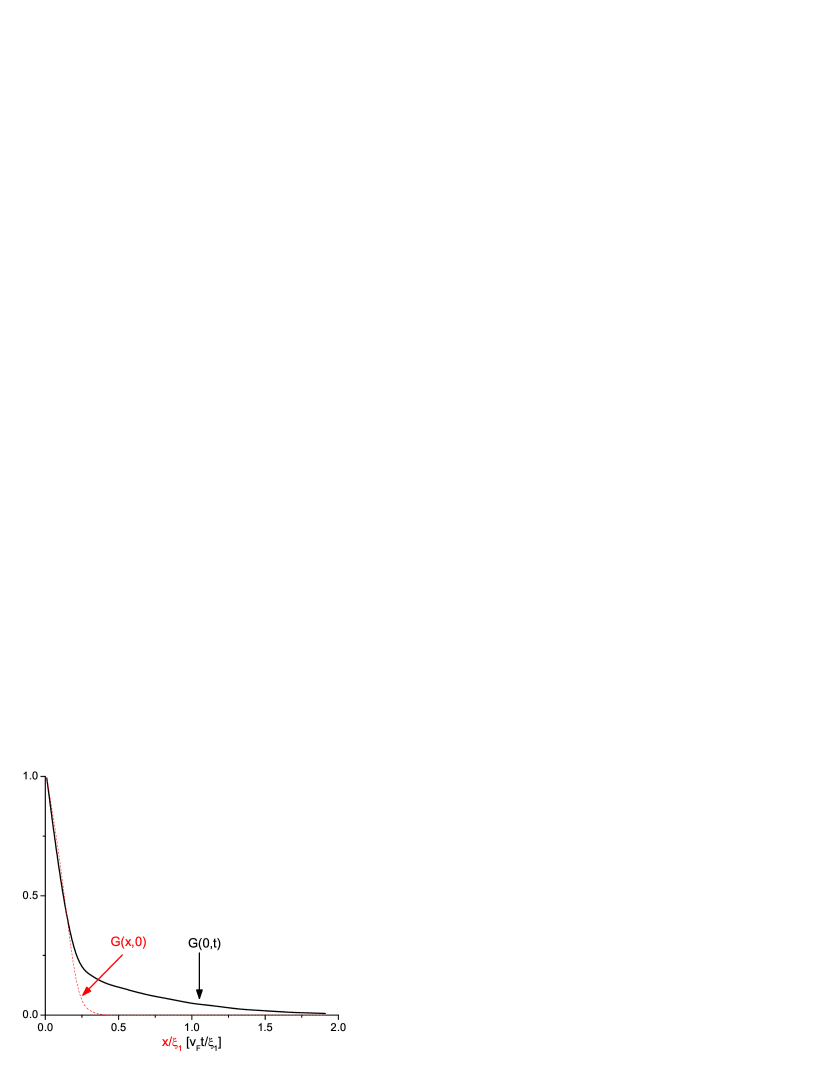
Figure 2: Plot of $G(x,0)$ (dashed line) and $G(0,t)$ (solid line) near the critical point ($r=0$) at $T=T_{1}$. The decay of $G(0,t)$ is slower than $G(x,0)$ as discussed in the text.

As we approach the critical point, $r\rightarrow 0$, and consequently one must retain the $b^{\prime}$ term, in the expression of $\gamma(q^{\prime})$. When $b^{\prime}\neq 0$, it is not possible to evaluate $Q$ analytically at finite temperature. However, since the electrons now see the critical bosonic fluctuations with dispersions $\omega\simeq q_{x}^{2}$, we expect the Green functions $G_{+}(x,0)$ and $G(0,t)$ to have different behavior. A plot of the Green functions shown in Figs. 2, confirms the above qualitative discussion. The characteristic scale of decay for $G(x,0)$ is seen to be much shorter compared to $G(0,t)$. This feature arises from the presence of critical fluctuations with $\omega\sim q_{x}^{2}$ dispersion ( in contrast to $\omega\sim q_{x}$ fluctuations in standard Luttinger liquid ) and is therefore a signature of the quantum critical point at finite temperature. We expect that a measurement of $\rho(\omega)$ and $n(k_{x})$ will probe this behavior.

IV Discussion

In this work, we have shown, by explicitly keeping track of the full SU(2) symmetry of the problem, that in 1D the Luttinger liquid to FM transition for Heisenberg ferromagnets has $z=2+{\rm O}(\epsilon^{2})$ in an $\epsilon$ expansion sense. The analysis done here was carried out at a Gaussian level, which is exact in 1D as long as the dispersion of the Fermions are linear. The curvature in Fermionic dispersion introduces quartic coupling terms beyond the Gaussian approximation. Although we have not carried out a full analysis of the problem with such coupling terms in the presence of the SU(2) symmetry, we have identified the typical quartic terms and discuss their consequences. In particular, we pointed out that for a ferromagnet with Ising symmetry, our analysis reduces to the standard Hertz-Millis theory. The Hertz-Millis approach is therefore completely equivalent to the bosonization approach of Ref. yang1, in 1D for Ising ferromagnets. In contrast, we find that for the Heisenberg ferromagnets, our theory does not reduce to that obtained by the traditional Hertz-Millis approach. We identify that this is due to additional coupling terms between the longitudinal and the transverse modes, shown in right panel of Fig. 1, which has no analog in the Ising case and are also different from the usual expected ${\bf m}^{4}$ interaction terms that one obtains using the Hertz-Millis approach. It will be interesting to carry out our analysis in higher dimension and compare the results with those of Ref. kirk, , where a possible problem with such ${\bf m}^{4}$ quartic terms in the usual Hertz-Millis approach has been discussed from a different point of view. A detailed analysis of this issue is left as a subject of future work.

We have also obtained an exact expression for the electron Green functions $G(x,0)$ and $G(0,t)$ for a range of finite temperature. Although we have not obtained the expression of the Green functions at the interacting fixed point, we hope that over a range of temperature where the properties of the system is expected to be well described by the Gaussian fixed point, $G(x,0)$ and $G(0,t)$ can be probed by experimentally accessible quantities such as the momentum distribution and tunneling DOS of the electrons.

This work was supported by NSERC of Canada, Canada Research Chair Program, and Canadian Institute for Advanced Research. We thank Kedar Damle, Dima Feldman, Subir Sachdev, and Kun Yang for their insightful comments and Eugene Kim for early collaboration on a related project.

References

• (1)
• (2) J.A. Hertz, Phys. Rev. B 14, 1165 (1976).
• (3) A.J. Millis, Phys. Rev. B 48, 7183 (1993).
• (4) D. Belitz and T.R. Kirkpatrick, Phys. Rev. Lett. 89, 247202 (2004).
• (5) E.H. Lieb and D. Mattis, Phys. Rev. 125, 164 (1962).
• (6) S. Daul and R.M. Noack, Phys. Rev. B 58, 2635 (1998).
• (7) L. Bartosch, M. Koller, and P. Kopietz, Phys. Rev. B 67, 092403 (2003).
• (8) K. Yang, Phys. Rev. Lett. 93, 066401 (2004).
• (9) S. Sachdev and T. Senthil, Annals of Physics 251, 76 (1996).
• (10) H.J Schulz in The Hubbard Model edited by D. Bareiswyl (Plenum, New York, 1995).
• (11) K. Sengupta and N. Dupuis , Phys. Rev. B 392, 151 (1998); K. Borejsza and N. Dupuis, Phys. Rev. B 69, 085119 (2004).
• (12) The procedure of obtaining a non-linear sigma model for a gapped quasi one-dimensional system is outlined in Ref.ย nicolas1, . We follow this procedure here and set the gap $\Delta$ to zero at the end of the calculation. However, this also means that the domain of validity of such the model, which is valid for $E<\Delta$, shrinks to zero. This implies that the coefficients of the model such as spin stiffness and susceptibility can not be trusted. As far as our analysis here is concerned, it does not depend on the precise values of these coefficients and is expected to hold as long as the coefficients remain non-singular. We do not know of any analysis which rigorously derives an effective model of spin fluctuation for a metallic system.
• (13) See, for instance, S. Sachdev, Quantum Phase Transitions (Cambridge University, Cambridge, England, 1999).
• (14) See, for instance, P. Kopietz, Bosonization of Interacting Fermions in Arbitrary Dimensions (Springer, Berlin, 1996).
• (15) X-G Wen and A. Zee, Phys. Rev. Lett. 61, 1025 (1988).
• (16) E. Witten, Nuclear Physics B 149, 285 (1979).
• (17) A. Dโ€™Adda, M. Luscher, and P. Di Vecchia, Nuclear Physics B 146, 63 (1978).
• (18) Note that to obtain ${\mathcal{K}}_{S}$, one proceeds exactly the same way as for ${\mathcal{S}}_{S}$. We first obtain ${\mathcal{K}}_{\alpha\alpha^{\prime}}=\left<j_{x\alpha}^{z}j_{x\alpha^{\prime}}^{z}\right>$ for $\alpha=R,L$, then switch over to the symmetric and antisymmetric modes $j_{x\,S(A)}^{z}=j_{x\,R}^{z}+(-)j_{x\,L}$ and finally integrate out the anti-symmetric modes to get ${\mathcal{K}}_{S}$.
• (19) The use of dressed, rather than the bare propagator of the gauge field is crucial here and can be justified as an attempt to take into account self-consistency of the problem. Of course, in general, it is not necessary that this procedure will lead to self-consistency. For the problem at hand, however, it can be checked a posteriori that the use of dressed propagator for the gauge fields indeed gives us a self-consistent solution in the infrared limit.
• (20) For Eq.ย 43 to hold, it is necessary that $J(q)$ is independent of the index $\alpha$. This point has been discussed in details in Ref.ย Kopietz, .
• (21) J. Schwinger, Phys. Rev. 128 2425 (1962).