Scale Invariance and Symmetry Relationships
In Non-Extensive Statistical Mechanics

Abstract

This article extends results described in a recent article detailing a structural scale invariance property of the simulated annealing (SA) algorithm. These extensions are based on generalizations of the SA algorithm based on Tsallis statistics and a non-extensive form of entropy. These scale invariance properties show how arbitrary aggregations of energy levels retain certain mathematical characteristics. In applying the non-extensive forms of statistical mechanics to illuminate these scale invariance properties, an interesting energy transformation is revealed that has a number of potentially useful applications. This energy transformation function also reveals a number of symmetry properties. Further extensions of this research indicate how this energy transformation function relates to power law distributions and potential application for overcoming the so-called “broken ergodicity” problem prevalent in many computer simulations of critical phenomena.

1 Introduction

Recent advances in statistical mechanics have helped to explain the behavior of large ensembles of interacting systems. Since the time of Boltzmann, there has been a great deal of effort in attempting to understand the behavior of such systems. In his day, a great deal of progress was made using a form of entropy that seemed to explain the behavior of the so-called “ideal gas” model, a model premised on the very limited form of interaction implied by elasticity assumptions. Notwithstanding these assumptions, it was able to predict, quite accurately, many attributes of the behavior of gases in thermal equilibrium.

Despite its enormous success for these idealized systems, the Boltzmann version of statistical mechanics has had limited success in explaining the behavior of more complex systems where the components interact in ways that are distinctly inelastic—that is to say, the particles do not obey simple Newtonian mechanics. In these models, the particles themselves may absorb energy during collisions in forms other than by changes in their velocity. The assumptions of the ideal gas model that these particles have no internal structure therefore cannot be assumed. Or, it may be that these particles exhibit attractive or repulsive forces between them. In any event, their gross behavior is not well predicted in systems governed by the Boltzmann-Gibbs entropy formula: $S_{BG}=-k\sum_{i=1}^{W}\pi_{i}\ln\pi_{i}$ where the $\pi_{i}$ represents the probability of the $i^{\mbox{\tiny th}}$ energy partition and $W$ represents the size (number of energy states) of the system. These complex systems obey various power laws and can exhibit phase transitions and related critical phenomena where there are drastic shifts in their energy configurations.

These power laws and criticality properties seem to be quite diverse and ubiquitous in nature. To help explain these behaviors, Tsallis [10, 11] developed a new entropy expression that forms the basis of a non-extensive form of thermodynamics:

$$S_{q}=\frac{k\left(1-\sum_{i=1}^{W}p_{i}^{q}\right)}{q-1}$$ (1)

where $k$ is a constant and $S_{q}$ is the entropy parameterized by the entropic parameter $q$. In classical statistical mechanics, entropy falls into a class of variables that are referred to as extensive because they scale with the size of the system. Intensive variables, such as temperature, do not scale with the size of the system . Tsallis’ form of entropy is non-extensive because the entropy of the union of two independent systems is not equal to the sum of the entropies of each system. That is, for independent systems $A$ and $B$,

$$S_{q}(A+B)=S_{q}(A)+S_{q}(B)+\frac{(1-q)S_{q}(A)S_{q}(B)}{k}$$ (2)

and Tsallis points out that $q=1$ recovers the extensivity properties of the Boltzmann-Gibbs entropy formula and further, that $\lim_{q\rightarrow 1}S_{q}=S_{BG}$, hence can be seen as a generalization of Boltzmann-Gibbs [10, 11]. Moreover, the stationary probabilities $p_{i}(t)$ of the system being in some $i$ further illustrates the generalization of the classic entropy form in that

$$\lim_{q\rightarrow 1}p_{i}(t)=\pi_{i}(t)$$ (3)

for all $t>0$ [10, p.483].

The entropic parameter $q$ controls important aspects of the probability distribution of the energy levels making it is possible to markedly change the nature of the thermodynamic system being modeled. For example, when $q>1$ the stationary probability distribution shifts from an exponential form to one with heavy tails that gives rise to a power law distribution, or conversely, one can increase the stationary probability of low energy states when $q<1$, something quite useful in optimization (see e.g., [1, 12]).

One of the best ways for studying the implications of this non-extensive form of statistical mechanics is through the use of computer simulations. The simulated annealing (SA) algorithm provides these basic simulation tools as it is, at heart, a simulation of a thermodynamic system although it has been used principally for solving optimization problems. Tsallis developed a generalized simulated annealing (GSA) algorithm [12] based on maximizing the entropy in (1).

Given these developments, it seems quite appropriate and useful to examine certain scale invariance properties [3] of the classic SA algorithm in light of the non-extensive form of entropy and the GSA. These scale invariance properties shed light on a number of behaviors and illustrate some curious effects on the configuration space itself. An energy transformation function is identified and used to illustrate a number of symmetry properties and potential applications. In addition, the behavior of parallel forms of SA, also exhibit scale invariance properties and can be used to illustrate certain analogies in the behavior of large ensembles of interacting particles or systems, a basic aspect of non-extensive statistical mechanical systems.

This article is organized as follows: Section 2 provides some background into non-extensive thermodynamics, simulated annealing, and SAs scale invariance properties. Section 3 develops the scale invariance properties of the non-extensive form of SA. These scale invariance properties indicate the existence of an energy transformation function. Section 5 describes certain asymptotic properties of this energy transformation function that suggest how it turns an exponential distribution into a power-law distribution. Section 6 provides some discussion on the implications of the scale invariance properties and the energy landscape transformation describes extensions of this work and directions for future research involving Markov Chain Monte Carlo simulation of complex systems.

2 Background

2.1 Non-Extensive Thermodynamics and Generalized SA

The GSA developed by Tsallis [12], entails a different form for the acceptance probabilities and stationary probabilities because of the form of (1), i.e., the stationary distribution is based on maximizing the value of $S_{q}$ rather than $S_{BG}$. The latter leads to the well-known Boltzmann-Gibbs distribution

$$\pi_{i}(t)=\frac{e^{-f_{i}/t}}{Z_{BG}}$$ (4)

where $Z_{BG}=\sum_{j=1}^{W}e^{-f_{j}/t}$ is the normalizing Boltzmann Partition Function. Note that because we will often be referring to the SA algorithm and the Metropolis Algorithm, the value of the “energy” function will be denoted by $f_{i}$ which is typically used in optimization problems to denote an objective function value, but this can also denote some energy value.

Maximizing the non-extensive entropy subject to certain constraints, described below, gives rise to a stationary probability distribution

$$p_{i}(t)=\frac{\left[1+\left(\frac{q-1}{t}\right)f_{i}\right]^{\frac{1}{1-q}}}{Z_{q}}$$ (5)

where $Z_{q}=\sum_{j=1}^{W}\left[1+\left(\frac{q-1}{t}\right)f_{j}\right]^{\frac{1}{1-q}}.$ Note that $p_{i}(t)$ will be used throughout to represent the stationary probability in the non-extensive case and $\pi_{i}(t)$ will represent the stationary probability in the classic, extensive case.

The definition of the stationary probability $p_{i}(t)$ in (5) is based on the particular set of constraints used in defining a thermodynamic system. Three distinct and noteworthy sets of constraints have been studied all of which employ the standard normalizing constraint $\sum_{i}p_{i}(t)=1$. What distinguishes these constraint sets is the relationships they define between probabilities and energy or objective function values. Tsallis [13] reports that different forms of these constraints have a number of implications for the non-extensive form of the probability $p_{i}(t)$. Here, the form defined by Tsallis’ Type 2 constraint [14] for GSA is used where,

$$\sum_{i=1}^{W}p_{i}^{q}f_{i}=U^{(2)},\mbox{ a constant},$$ (6)

whereas in his original paper, the constraint $\sum_{i}\tilde{p}_{i}f_{i}=U$ was used. This later constraint was referred to as the Type 1 constraint in [13, p. 537] and leads to a different stationary probability denoted here by $\tilde{p}_{i}$. It bears emphasis that the limit in (3) holds for all the different stationary probabilities that arise from the use of the different constraints [13]. Initially, the notions of scale invariant structures will be based on the Type 2 constraint and then later, in a more useful context, the scale invariance of the Type 1 constraint will be examined.

2.2 Classical SA Scale Invariance

Among the many interesting aspects of the SA and Metropolis algorithms is a scale invariance property associated with the stationary probabilities of various states. This scale invariance property is manifest in the identical mathematical forms of certain quantities involving individual states, aggregated states of the solution space, and the aggregation of states associated with multiple processors in an expanded state space. See [3, 4] for a complete description.

One aspect of this scale invariance involves the rate change of the stationary probability of a state $i$ with respect to temperature $t$:

$$\frac{\partial\pi_{i}(t)}{\partial t}=\frac{\pi_{i}(t)}{t^{2}}\left[f_{i}-\langle f\rangle(t)\right]$$ (7)

where $\langle f\rangle(t)$ is the expected objective function value at temperature $t$. For aggregated states $A=\{i_{1},i_{2},\ldots,i_{m}\}$, define

$$\pi_{A}(t)\equiv\sum_{i\in A}\pi_{i}(t),\ \ f_{A}(t)\equiv\frac{\sum_{i\in A}\pi_{i}(t)f_{i}}{\pi_{A}(t)},$$ (8)

the conditional expectation of the objective function value given that the current state is in set $A$ (see [3, p.224] for a more complete treatment). It then follows that

$$\frac{\partial\pi_{A}(t)}{\partial t}=\frac{\pi_{A}(t)}{t^{2}}\left[f_{A}(t)-\langle f\rangle(t)\right]$$ (9)

where the similarity of (7) and (9) indicates a form of scale invariance.

Scale invariance also extends to second moments. For standard SA,

$$\frac{\partial\langle f\rangle(t)}{\partial t}=\frac{\partial f_{\Omega}(t)}{\partial t}=\frac{\sigma^{2}_{\Omega}(t)}{t^{2}}$$ (10)

where $\sigma^{2}_{\Omega}(t)$ represents the variance over the entire solution space at temperature $t$. Scale invariance is exhibited by the fact that

$$\frac{\partial f_{A}(t)}{\partial t}=\frac{\sigma^{2}_{A}(t)}{t^{2}}$$ (11)

and $\sigma_{A}^{2}(t)$ is the variance of objective function values at temperature $t$ conditioned on the current state being in set $A$. See [3, p.232-33] for details.

3 SA Scale Invariance with Non-Extensive Entropy

3.1 The Basis of Scale Invariance

To demonstrate scale invariance based on aggregated states in the non-extensive case, a basis for making comparisons must be established. To that end, the following temperature derivative of $p_{i}(t)$ is calculated for the non-extensive SA case. For notational convenience, simplicity and to ensure positivity, let $N_{i}(t)\equiv\left[1+\left(\frac{q-1}{t}\right)f_{i}\right]^{\frac{1}{1-q}}$ (hereinafter we will drop the $(t)$ from $N_{i}(t)$ to further simplify the expressions) and taking the derivative of (5),

$$\frac{\partial p_{i}(t)}{\partial t}=\frac{Z_{q}\frac{\partial}{\partial t}N_{i}-N_{i}\frac{\partial}{\partial t}Z_{q}}{(Z_{q})^{2}}.$$ (12)

Note that

$$\frac{\partial N_{i}}{\partial t}=\frac{\partial}{\partial t}\left[1+\left(\frac{q-1}{t}\right)f_{i}\right]^{\frac{1}{1-q}}=\frac{f_{i}N_{i}^{q}}{t^{2}},$$ (13)

$Z_{q}=\sum_{j}N_{j},$ and $\ p_{i}(t)=N_{i}/Z_{q}$ and hence

$$\frac{\partial}{\partial t}Z_{q}=\frac{\partial}{\partial t}\sum_{j}N_{j}=\sum_{j}\frac{\partial N_{j}}{\partial t}=\sum_{j}\frac{f_{j}N_{j}^{q}}{t^{2}}.$$

Substituting this and (13) into (12) yields

$$\frac{\partial p_{i}(t)}{\partial t} = \frac{\left(\sum_{j}N_{j}\right)\frac{f_{i}N^{q}_{i}}{t^{2}}-\frac{N_{i}}{t^{2}}\sum_{j}f_{j}N_{j}^{q}}{(\sum_{j}N_{j})^{2}}$$ (14)

$$= \frac{p_{i}(t)f_{i}N_{i}^{q-1}}{t^{2}}-\frac{p_{i}(t)\sum_{j}f_{j}N_{j}^{q}}{t^{2}\sum_{j}N_{j}}$$

$$= \frac{p_{i}(t)}{t^{2}}\left[f_{i}N_{i}^{q-1}-\frac{\sum_{j}f_{j}N_{j}^{q}}{\sum_{j}N_{j}}\right]$$

To further simplify and clarify, define

$$\hat{f}_{i}(f_{i},q,t)\equiv f_{i}N_{i}^{q-1}=\frac{f_{i}}{1+\left(\frac{q-1}{t}\right)f_{i}}$$ (15)

and will often be denoted simply by $\hat{f}_{i}$ or $\hat{f}_{i}(t)$ where it is understood to involve $f_{i},q$ and $t$. Substituting (15) into (14) and further simplifying yields

$$\frac{\partial p_{i}(t)}{\partial t}=\frac{p_{i}(t)}{t^{2}}\left[\hat{f}_{i}(t)-\langle\hat{f}\rangle(t)\right]$$ (16)

and which interestingly enough is analogous to (7). Notice that for $q=1,\ \hat{f}_{i}(t)=f_{i},\ \forall\ t>0$. Tsallis [10, 11] established that $\lim_{q\rightarrow 1}p_{i}(t)=\pi_{i}(t)$, hence, in the limit as $q\rightarrow 1$, (16) $\rightarrow$ (7). The symbol $\hat{f_{i}}(t)$ will be referred to as the $q$-transformation of $f_{i}$. Later on, some interesting properties of this transformation will be examined.

3.2 Scale Invariance from the Aggregation of States

In similar fashion as in [3], define $p_{A}(t)=\sum_{i\in A}p_{i}(t)$ for $A\subset\Omega$, where $\Omega$ is the set of microstates and where $W=|\Omega|$ and

$$\hat{f}_{A}(t)=\frac{\sum_{i\in A}p_{i}(t)\hat{f}_{i}(t)}{p_{A}(t)},$$ (17)

the conditional expectation of $\hat{f}_{i}(t)$ conditioned on the current state being in set $A$. Taking the derivative,

$$\frac{\partial p_{A}(t)}{\partial t}=\frac{\partial}{\partial t}\sum_{i\in A}p_{i}(t)=\sum_{i\in A}\frac{\partial p_{i}(t)}{\partial t}.$$ (18)

Substituting (16) and (17) into (18) yields

$$\frac{\partial p_{A}(t)}{\partial t} = \sum_{i\in A}\frac{p_{i}(t)}{t^{2}}\left[\hat{f}_{i}(t)-\langle\hat{f}\rangle(t)\right]$$ (19)

$$= \sum_{i\in A}\frac{p_{i}(t)\hat{f}_{i}(t)}{t^{2}}-\sum_{i\in A}\frac{p_{i}(t)\langle\hat{f}\rangle(t)}{t^{2}}$$

$$= \frac{p_{A}(t)}{t^{2}}\sum_{i\in A}\frac{p_{i}(t)\hat{f}_{i}(t)}{p_{A}(t)}-\frac{p_{A}(t)\langle\hat{f}\rangle(t)}{t^{2}}$$

$$= \frac{p_{A}(t)}{t^{2}}\left[\hat{f}_{A}(t)-\langle\hat{f}\rangle(t)\right]$$

where for aggregated states, (19) has a similar mathematical structure as (16), hence exhibits a scale invariance property the foundation of which is based on the energy transformation function $\hat{f}_{i}(f_{i},q,t)$.

3.2.1 Scale Invariance in Second Moments

Scale invariance in the non-extensive form of SA for second moments is indicated in the following where again the $q$-transformation of $f_{i}$ and $f_{A}(t)$ is used. First, the parallels to the classic case is illustrated. Thus,

$$\frac{\partial\langle\hat{f}\rangle(t)}{\partial t} = \frac{\partial\hat{f}_{\Omega}(t)}{\partial t}=\frac{\partial}{\partial t}\left[\sum_{i\in\Omega}p_{i}(t)\hat{f}_{i}(t)\right]$$ (20)

$$= \sum_{i\in\Omega}\frac{\partial}{\partial t}\left[p_{i}(t)\hat{f}_{i}(t)\right]$$

$$= \sum_{i\in\Omega}\left[\frac{\partial p_{i}(t)}{\partial t}\hat{f}_{i}(t)+p_{i}(t)\frac{\partial\hat{f}_{i}(t)}{\partial t}\right].$$

Substituting (16) into the first part of (20) and simplifying yields

$$\frac{\partial\langle\hat{f}\rangle(t)}{\partial t}=\sum_{i\in\Omega}\frac{p_{i}(t)\hat{f}^{2}_{i}(t)}{t^{2}}-\sum_{i\in\Omega}\frac{\hat{f}_{\Omega}(t)p_{i}(t)\hat{f}_{i}(t)}{t^{2}}+\sum_{i\in\Omega}p_{i}(t)\frac{\partial\hat{f}_{i}(t)}{\partial t}.$$ (21)

Noting the form of the first two terms in (21) and the fact that in the third term

$$\frac{\partial\hat{f}_{i}(t)}{\partial t}=\left(\hat{f}_{i}(t)\right)^{2}\left(\frac{q-1}{t^{2}}\right)$$ (22)

and substituting into (21) and dropping the $(t)$ for notational clarity and adding the symbol $\Omega$ to denote expectations over the entire state space yields

$$\frac{\partial{\langle\hat{f}\rangle}_{\Omega}}{\partial t} = \frac{{\langle\hat{f}^{2}\rangle}_{\Omega}-{\langle\hat{f}\rangle}_{\Omega}^{2}+(q-1){\langle\hat{f}^{2}\rangle}_{\Omega}}{t^{2}}$$ (23)

$$= \frac{\hat{\sigma}_{\Omega}^{2}}{t^{2}}+\frac{(q-1){\langle\hat{f}^{2}\rangle}_{\Omega}}{t^{2}}$$

where $\hat{\sigma}_{\Omega}^{2}$ represents the variance of the $q$-transformed objective function values over the entire objective function space (at temperature $t$). Obviously, this expression is slightly different from the classic SA case as indicated in (10). Note that $\lim_{q\rightarrow 1}\hat{\sigma}_{\Omega}^{2}=\sigma_{\Omega}^{2}$ so that the expressions in (23) and (10) become equivalent.

The expression in (23) quite clearly shows the effects of the value of $q$—values greater (less) than 1 increase (decrease) the rate of change of the expected objective function values ($q$-transformed values). Eq. (23) also provides the basis for another form of scale invariance. Thus, after going through similar steps as in (20) through (23) we get

$$\frac{\partial\hat{f}_{A}}{\partial t}=\frac{\sum_{i\in A}p_{i}\hat{f}_{i}^{2}}{t^{2}p_{A}}-\frac{\hat{f}_{A}^{2}}{t^{2}}+\left(\frac{q-1}{t^{2}}\right)\frac{\sum_{i\in A}p_{i}\hat{f}^{2}_{i}}{p_{A}}.$$ (24)

Noting that the first and third terms indicate conditional expectations conditioned on the current state being in set $A$, then (24) can be re-written in the convenient notation

$$\frac{\partial\hat{f}_{A}}{\partial t} = \frac{{\langle\hat{f}^{2}\rangle}_{A}-{\langle\hat{f}\rangle}_{A}^{2}+(q-1){\langle\hat{f}^{2}\rangle}_{A}}{t^{2}}$$ (25)

$$= \frac{\hat{\sigma}^{2}_{A}}{t^{2}}+\frac{(q-1){\langle\hat{f}^{2}\rangle}_{A}}{t^{2}}$$

where (25) is clearly analogous to (23) and so exhibits a form of scale invariance. Again, in the limit as $q\rightarrow 1$ both of these equations correspond to the scale invariance of standard (Boltzmann-Gibbs) SA as indicated in (10) and (11). What is interesting however is the fact that the terms involving $(q-1)$ also scale with the aggregated set $A$ in the non-extensive case.

3.3 Scale Invariance from the Aggregation of Processors

3.3.1 The Classic SA Case

Fleischer [5, 6, 7] describes another form of scale invariance based on the aggregation parallel and independent processes each running the SA algorithm independently of one another. This type of aggregation contrasts sharply with the aggregation of states and hence directly affects the nature of the scale invariance and how the algorithm itself functions. In this respect, one may view the SA algorithm as a single processor or particle that probabilistically visits a single state at each iteration of the algorithm. Thus, when a set of states is aggregated and fixed, the particle visits the aggregated state probabilistically and in a way that dictates how the stationary probability and objective function value should reasonably be defined, i.e., based on the sum of the stationary probabilities and the conditional expectation of the objective function respectively as given in (8).

In aggregating $p$ independent processors however, the state space $\Omega$ becomes $\Omega^{p}$ and the stationary probability and objective function values associated with the set of processors must be defined differently and requires the following definitions. First, define a state in the product space spanned by $p$ processors as $i_{1}i_{2}\ldots i_{p}$. In classic SA scale invariance

$$\pi_{i_{1}i_{2}\ldots i_{p}}(t)=\prod_{m=1}^{p}\pi_{i_{m}}(t)$$ (26)

and is based on the concept of the joint probability of independent processors. Similarly, the objective function associated with a set of $p$ independent particles is simply the sum of each particle’s objective function value as opposed to the conditional expectation, and defined by

$$f_{i_{1}i_{2}\ldots i_{p}}\equiv\sum_{m=1}^{p}f_{i_{m}}.$$

Scale invariance is indicated by

$$\pi_{i_{1}i_{2}\ldots i_{p}}(t)=\frac{e^{-f_{i_{1}i_{2}\ldots i_{p}}/t}}{\sum_{j_{p}}\cdots\sum_{j_{1}}e^{-f_{j_{1}j_{2}\ldots j_{p}}/t}}$$

(see [3, 6]) which has the same form as (4) and the fact that the temperature derivative is proportional to the difference between a function of the objective function value and its expectation:

$$\frac{\partial\pi_{i_{1}i_{2}\ldots i_{p}}(t)}{\partial t}=\frac{\pi_{i_{1}i_{2}\ldots i_{p}}(t)}{t^{2}}\left[f_{i_{1}i_{2}\ldots i_{p}}-{\langle f\rangle}_{\Omega^{p}}(t)\right]$$ (27)

[3, p.222] where the expectation is over all the states of the product space.

3.3.2 The Non-Extensive SA Case

Taking cues from this earlier work, define the stationary probability of state $i_{1}i_{2}\ldots i_{p}$ spanned by $p$ independent processors and based on the Tsallis entropy by

$$p_{i_{1}i_{2}\ldots i_{p}}(t)\equiv\prod_{m=1}^{p}p_{i_{m}}(t).$$

Simplifying using the case of $p=2$ (the following expressions are readily extended to the more general case) and letting $a=(q-1)/t$ for notational clarity, the joint probability of a state $i_{1}i_{2}$ is

$$p_{i_{1}i_{2}}(t) = \frac{[1+af_{i_{1}}]^{\frac{1}{1-q}}[1+af_{i_{2}}]^{\frac{1}{1-q}}}{Z_{q}^{2}}$$ (28)

$$= \frac{[1+a(f_{i_{1}}+f_{i_{2}}+af_{i_{1}}f_{i_{2}})]^{\frac{1}{1-q}}}{Z_{q}^{2}}$$

$$= \frac{[1+a\tilde{f}_{i_{1}i_{2}}(t)]^{\frac{1}{1-q}}}{Z_{q}^{2}}$$

where $\tilde{f}_{i_{1}i_{2}}(t)\equiv f_{i_{1}}+f_{i_{2}}+af_{i_{1}}f_{i_{2}}$ and where it is also the case that

$$Z_{q}^{2} = \left(\sum_{i=1}^{W}\left[1+af_{i}\right]^{\frac{1}{1-q}}\right)^{2}$$

$$= \sum_{i_{1}=1}^{W}\sum_{i_{2}=1}^{W}\left[1+a\tilde{f}_{i_{1}i_{2}}(t)\right]^{\frac{1}{1-q}}.$$

Thus, the form of $p_{i_{1}i_{2}}(t)$ in the product space closely follows that of $p_{i}(t)$ with the advantage that the non-extensivity property is exemplified by $\tilde{f}_{i_{1}i_{2}}(t)$ which is somewhat similar to the entropy relationships in (2). Note that for $q=1,\ \tilde{f}_{i_{1}i_{2}}(t)=f_{i_{1}i_{2}}=f_{i_{1}}+f_{i_{2}}$ for all $t$. Thus, in the limit as $q\rightarrow 1$, (28) is equivalent to the Boltzmann-Gibbs case in (26) (recall (3)).

Examining the derivative of the stationary probability using (16) also reflects a scale invariance property and yields

$$\frac{\partial p_{i_{1}i_{2}}(t)}{\partial t} = \frac{\partial}{\partial t}\left[p_{i_{1}}\kern-2.0pt(t)p_{i_{2}}\kern-2.0pt(t)\right]$$

$$= p_{i_{1}}\kern-2.0pt(t)\frac{p_{i_{2}}\kern-2.0pt(t)}{t^{2}}\left[\hat{f}_{i_{2}}-{\langle\hat{f}\rangle}_{\Omega}\right]$$

$$\hskip 10.0pt+p_{i_{2}}\kern-2.0pt(t)\frac{p_{i_{1}}\kern-2.0pt(t)}{t^{2}}\left[\hat{f}_{i_{1}}-{\langle\hat{f}\rangle}_{\Omega}\right]$$

$$= \frac{p_{i_{1}i_{2}}\kern-2.0pt(t)}{t^{2}}\left[\hat{f}_{i_{1}i_{2}}-{\langle\hat{f}\rangle}_{\Omega^{2}}\right]$$

and in general it follows that

$$\frac{\partial p_{i_{1}\cdots i_{p}}\kern-2.0pt(t)}{\partial t}=\frac{p_{i_{1}\cdots i_{p}}\kern-2.0pt(t)}{t^{2}}\left[\hat{f}_{i_{1}\cdots i_{p}}-{\langle\hat{f}\rangle}_{\Omega^{p}}\right]$$ (29)

where $\hat{f}_{i_{1}\cdots i_{p}}=\sum_{m=1}^{p}\hat{f}_{i_{m}}$ and ${\langle\hat{f}\rangle}_{\Omega^{p}}=p{\langle\hat{f}\rangle}_{\Omega}$ and equals the expectation of $\hat{f}_{i_{1}\cdots i_{p}}$. Note that (29) again has a factor equal to the difference between a function of the objective function values and its expectation and has the same structure as in (7), (9), (16), (19) and (27).

Finally, let us examine the temperature derivative of ${\langle\hat{f}\rangle}_{\Omega^{p}}$ and see how it compares to (23) and (25). Thus,

$$\frac{\partial{\langle\hat{f}\rangle}_{\Omega^{p}}}{\partial t}=\frac{\partial}{\partial t}\sum_{i_{1}\cdots i_{p}}p_{i_{1}\cdots i_{p}}\kern-2.0pt(t)\hat{f}_{i_{1}\cdots i_{p}}\kern-2.0pt(t).$$

Using the results from (20) through (22) and noting that $\hat{f}_{i_{1}\cdots i_{p}}(t)$ is a sum of terms,

$$\frac{\partial\hat{f}_{i_{1}\cdots i_{p}}}{\partial t}=\left(\frac{q-1}{t^{2}}\right)\sum_{m=1}^{p}\hat{f}_{i_{m}}^{\kern 1.5pt2}=\left(\frac{q-1}{t^{2}}\right)\hat{f}_{i_{1}\cdots i_{p}}^{\kern 1.5pt2}$$

yields

$$\frac{\partial{\langle\hat{f}\rangle}_{\Omega^{p}}}{\partial t} = \frac{{\langle\hat{f}^{2}\rangle}_{\Omega^{p}}-{\langle\hat{f}\rangle}^{2}_{\Omega^{p}}+(q-1){\langle\hat{f}^{2}\rangle}_{\Omega^{p}}}{t^{2}}$$ (30)

$$= \frac{\hat{\sigma}_{\Omega^{p}}^{2}}{t^{2}}+\frac{(q-1){\langle\hat{f}^{2}\rangle}_{\Omega^{p}}}{t^{2}}$$

where $\hat{\sigma}^{2}_{\Omega^{p}}$ represents the variance of the sums $\hat{f}_{i_{1}\cdots i_{p}}(t)$ (again, bear in mind that the dependence on $t$ is not indicated). Eq. (30) has the same form as (20) and (25) indicating a form of scale invariance. What is remarkable however is that in aggregating processors, the objective function is defined as the sum of the objective function values of each processor whereas in aggregating states, the objective function is defined as the conditional expectation of objective functions, yet they have the same form and in the limit as $q\rightarrow 1$ are equivalent to the aggregation of processors in classic SA.

3.4 Consistency

Fleischer [3] describes the concept of consistency in the scale invariant structure of SA based on the definition of the aggregated objective function $f_{A}$. This consistency property states that one can use identical means to define the objective function (here we describe it in terms of an energy level) associated with the aggregation of two or more aggregated states $A$ and $B$. Thus,

$$f_{A\cup B}(t) = \sum_{i\in A\cup B}\frac{\pi_{i}(t)f_{i}}{\pi_{A\cup B}(t)}$$

$$= \sum_{i\in A}\frac{\pi_{i}(t)f_{i}}{\pi_{A\cup B}(t)}+\sum_{i\in B}\frac{\pi_{i}(t)f_{i}}{\pi_{A\cup B}(t)}$$

$$= \frac{\pi_{A}(t)f_{A}(t)+\pi_{B}(t)f_{B}(t)}{\pi_{A}(t)+\pi_{B}(t)}$$

The definition of the objective function for state $A\cup B$ has the same form as the definition of aggregated states $A$ and $B$ and thus the scaling phenomenon in these definitions is, indeed, invariant on all levels of scale. It is easy to see that this same consistency property holds for the transformed objective function (energy level) $\hat{f}_{A\cup B}$ based on values $\hat{f}_{A}$ and $\hat{f}_{B}$ in the non-extensive case. In non-extensive systems however, the concept of consistency extends a bit further than in the classical case because of the energy transformation function.

The alert reader may have wondered, for example, if the definition of $\hat{f}_{A}(t)$ for some aggregation of energy levels $A$ defined in (17) could be equated to the $q$-transformation of some value $f_{A}(t)$ obtained by the weighted average of the untransformed values $f_{i}$. In other words,

$$\hat{f}_{A}\ =\ \frac{\sum_{i\in A}p_{i}\hat{f}_{i}}{p_{A}}\ \stackrel{{\scriptstyle?}}{{=}}\ \frac{f_{A}}{1+af_{A}}.$$ (31)

where

$$f_{A}=\frac{\sum_{i\in A}p_{i}f_{i}}{p_{A}}.$$ (32)

In general, the weighted sum of transformed energy values is not equal to the transformation of the weighted sum of energy values. The exception is when $q=1$ or the temperature is infinite for then $a=0$ and $\hat{f}_{A}=f_{A}$ and $p_{A}=\pi_{A}$ and the notion of consistency described in [3] holds because the relationships here are in effect the same as in [3]. The following theorem shows that these quantities are approximately equal for any given finite temperature for values of $f_{i}>0$ or $a>0$ sufficiently high.

Theorem 1

Let $\hat{f}_{A}$ and $f_{A}$ be defined as in (31) and (32), respectively with $a>0$. Then for values of $f_{i\in A}$ or $a$ sufficiently high,

$$\hat{f}_{A}\ \approx\ \frac{f_{A}}{1+af_{A}}.$$

Proof:
This statement is proved by showing that for any $\epsilon>0$, there is an energy value $f^{*}=\displaystyle\min_{i\in A}\{f_{i}\}$ or an $a>0$ sufficiently high such that

$$\left|\frac{\sum_{i\in A}p_{i}\hat{f}_{i}}{p_{A}}-\frac{f_{A}}{1+\,af_{A}}\right|<\epsilon.$$ (33)

For notational clarity, let $\omega_{i}=\frac{p_{i}}{p_{A}}$ and hence $\sum_{i\in A}\omega_{i}=1$. Rewriting (33) and taking the limit as $f^{*}\rightarrow\infty$ we obtain

$$\lim_{f^{*}\rightarrow\infty}\left|\sum_{i\in A}\frac{\omega_{i}f_{i}}{1+af_{i}}-\frac{\sum_{i\in A}\omega_{i}f_{i}}{1+\,a\sum_{i\in A}\omega_{i}f_{i}}\right|$$

$$= \left|\lim_{f^{*}\rightarrow\infty}\left(\sum_{i\in A}\frac{\omega_{i}f_{i}}{1+af_{i}}-\frac{\sum_{i\in A}\omega_{i}f_{i}}{1+\,a\sum_{i\in A}\omega_{i}f_{i}}\right)\right|$$

$$= \left|\left(\lim_{f^{*}\rightarrow\infty}\sum_{i\in A}\frac{\omega_{i}}{\frac{1}{f_{i}}+a}\right)-\left(\lim_{f^{*}\rightarrow\infty}\frac{1}{\left(\frac{1}{\sum_{i\in A}\omega_{i}f_{i}}\right)+\,a}\right)\right|$$

$$= \left|\frac{1}{a}-\frac{1}{a}\right|=0$$

since for all $i\in A,f_{i}\geq f^{*}$. For $a>0$ sufficiently high, both terms have limits of zero. Consequently, for all $\epsilon>0$, there exists an $f^{*}$ or $a>0$ such that (33) holds.  $\blacksquare$

Theorem 1 shows that in the high energy regions of the energy landscape it makes no significant difference if energy levels are aggregated first to obtain the value of $f_{A}$ and then transforming that value to obtain $\hat{f}_{A}$ or we transform the values $f_{i}$ first to obtain the $\hat{f}_{i}$ and then aggregate them to obtain $\hat{f}_{A}$—either way, they both yield values close to $1/a$.

4 Symmetry Relationships

Tsallis observes a symmetry relationship in using the different constraints described earlier in Section 2 and in text surrounding (6) [13]. Tsallis’ original incarnation of non-extensivity was based on his Type 1 constraint $\sum_{i}\tilde{p}_{i}f_{i}=U^{(1)}$ (see [13]) for stationary probability

$$\tilde{p}_{i}(t)=\frac{\left[1+\left(\frac{1-q}{t}\right)f_{i}\right]^{\frac{1}{q-1}}}{Z_{q}^{\prime}}$$ (34)

where $Z_{q}^{\prime}$ is the obvious normalizing constant (in physics nomenclature, the $U^{(1)}$ refers to the expected value of the eigenvalues of the Hamiltonian of the system although here, we can simply refer to it as the expected value of some energy). Tsallis points out that the form of $\tilde{p}_{i}$ is essentially the same as that of $p_{i}(t)$ except that $1-q$ replaces every occurrence of $q-1$ and vice versa including in the exponents (compare (34) with (5)). This interesting fact provides hints of additional symmetry relationships. In this section, these types of symmetry relationships are further explored in light of the scale invariance properties already developed.

4.1 Scale Invariance Using Other Constraints

It is quite reasonable to ask whether the constraint $\sum_{i}\tilde{p}_{i}f_{i}=U^{(1)}$ also leads to scale invariant forms and other symmetry relationships such as those described above. Define the energy transformation

$$\tilde{f}_{i}(f_{i},q,t)\equiv\frac{f_{i}}{1+\left(\frac{1-q}{t}\right)f_{i}}=\frac{f_{i}}{1-af_{i}}$$ (35)

where, for convenience, we use the earlier definition of $a$ and will often denote this as simply $\tilde{f}_{i}$. Using the same approach as in equations (12) through (16) we obtain

$$\frac{\partial\tilde{p}_{i}(t)}{\partial t}=\frac{\tilde{p}_{i}(t)}{t^{2}}\left[\tilde{f}_{i}(t)-\langle\tilde{f}\rangle(t)\right]$$

which again, using the same arguments on the aggregation of states, leads to

$$\frac{\partial\tilde{p}_{A}(t)}{\partial t}=\frac{\tilde{p}_{A}(t)}{t^{2}}\left[\tilde{f}_{A}(t)-\langle\tilde{f}\rangle(t)\right].$$

Note that the only difference between this and the earlier result is that every occurrence of $p_{i}$ and $\hat{f}_{i}$ is replaced with a $\tilde{p}_{i}$ and $\tilde{f}_{i}$, respectively.

4.1.1 Second Moments

Proceeding in the same fashion as in (20) through (25) we obtain the result

$$\frac{\partial{\langle\tilde{f}\rangle}_{\Omega}}{\partial t} = \frac{{\langle\tilde{f}^{2}\rangle}_{\Omega}-{\langle\tilde{f}\rangle}_{\Omega}^{2}+(1-q){\langle\tilde{f}^{2}\rangle}_{\Omega}}{t^{2}}$$ (36)

$$= \frac{\tilde{\sigma}_{\Omega}^{2}}{t^{2}}+\frac{(1-q){\langle\tilde{f}^{2}\rangle}_{\Omega}}{t^{2}}.$$

Scale invariance in second moments with the Tsallis constraint Type 1 is indicated by

$$\frac{\partial\tilde{f}_{A}}{\partial t} = \frac{{\langle\tilde{f}^{2}\rangle}_{A}-{\langle\tilde{f}\rangle}_{A}^{2}+(1-q){\langle\tilde{f}^{2}\rangle}_{A}}{t^{2}}$$ (37)

$$= \frac{\tilde{\sigma}^{2}_{A}}{t^{2}}+\frac{(1-q){\langle\tilde{f}^{2}\rangle}_{A}}{t^{2}}$$

where (36) and (37) are similar to (23) and (25) except that, as before, every occurrence of $q-1$ and $\hat{f}$ has been replaced with a $1-q$ and $\tilde{f}$, respectively.

4.2 Probabilities and Energy Relations

A number of additional forms of symmetry become evident when we examine the various relationships between probabilities and transformed energy values. First, suppose we wish to define $p_{i}(t)$ in terms of $\hat{f}_{i}$. Using the energy transformation function in (15) it is easy to see that

$$f_{i}=\frac{\hat{f}_{i}}{1+\left(\frac{1-q}{t}\right)\hat{f}_{i}}=\frac{\hat{f}_{i}}{1-a\hat{f}_{i}}$$ (38)

where again we use $a=\left(\frac{q-1}{t}\right)$ for notational convenience. Note that the $q-1$ in (15) has been replaced with $1-q$ in (38).

Note that (35) has a similar form as (38) where $f_{i}$ is defined in terms of $\hat{f}_{i}$, and hence it follows that

$$f_{i}=\frac{\tilde{f}_{i}}{1+\left(\frac{q-1}{t}\right)\tilde{f}_{i}}=\frac{\tilde{f}_{i}}{1+a\tilde{f}_{i}}$$

and has the same form as the definition of $\hat{f}_{i}$ in (15).

Now, substituting (38) into the form for $p_{i}(t)$ in (5), we get

$$p_{i}(t) = \frac{\left[1+a\left(\frac{\hat{f}_{i}}{1-a\hat{f}_{i}}\right)\right]^{\frac{1}{1-q}}}{Z_{q}}$$

$$= \frac{\left[\frac{1}{1-a\hat{f}_{i}}\right]^{\frac{1}{1-q}}}{Z_{q}}$$

$$= \frac{\left[1+\left(\frac{1-q}{t}\right)\hat{f}_{i}\right]^{\frac{1}{q-1}}}{Z_{q}}$$

which, interestingly, is exactly the same form as in (34) above where the Type 1 constraint was used. This also clearly implies that

$$Z_{q}=\sum_{i=1}^{W}\left[1+\left(\frac{q-1}{t}\right)f_{i}\right]^{\frac{1}{1-q}}$$

$$= \sum_{i=1}^{W}\left[1+\left(\frac{1-q}{t}\right)\hat{f}_{i}\right]^{\frac{1}{q-1}}$$

which further suggests another important relationship described below. Before this relationship is shown, however, a little more background into the use of other constraints is in order.

The expression $p^{q}_{i}$ arise in a number of instances, in particular, in the definition of $S_{q}$ itself and so has a very fundamental character. It also arises in other fundamental relationships concerning conditional probabilities and Shannon Additivity (see [2]). It also became evident that it was useful to incorporate them in the constraints that define the stationary probability. The “first choice” using Tsallis’ notation, $\sum_{i}\tilde{p}_{i}f_{i}=U^{(1)}$ lead to problems. The “second choice”, i.e., $\sum_{i}p^{q}_{i}f_{i}=U^{(2)}$ resolved some of them. Tsallis summarizes:

The first choice was very little used in the literature because quite quickly it became obvious that it could not solve relevant mathematical difficulties existing in the approach of anomalous phenomena such as Lévy superdiffusion. The second choice has been profusely used in the literature, and was not quickly abandoned because the deep physical reason for the generalization $(q\neq 1)$ was not transparent. But, in the light of recent developments [ ] showing the relationship of the formalism with a possible violation of the usual ergodic mixing hypothesis, features like the $q$-expectation value of unity not being equal to one became clearly unacceptable. Then naturally emerged the third choice, which we believe to be fully satisfactory…

[13]. We leave the implications of the third choice to future efforts.

Tsallis notes the effects of the exponent $q$ in the type 2 constraint as they “[privilegiate] the rare and the frequent events” depending on whether $q<1$ or $q>1$, respectively [13, p.535]. But this notion of shifting the probability weight of different energy values is, in some sense, equivalent to transforming the energy values themselves as the following lemma illustrates.

Lemma 1

For all $q>1$,

$$\sum_{i}p^{q}_{i}f_{i}=Z_{q}^{1-q}\sum_{i}p_{i}\hat{f}_{i}=Z_{q}^{1-q}\langle\hat{f}\rangle.$$

Proof:
It follows from the definition of $p_{i}$, that for all $i$,

$$p^{q}_{i}f_{i}=\left(\frac{\left[1+\left(\frac{q-1}{t}\right)f_{i}\right]^{\frac{1}{1-q}}}{Z_{q}}\right)^{q}f_{i}.$$ (39)

Now observe that $\frac{q}{1-q}=\frac{1}{1-q}-1$. Consequently for all $i$,

$$p_{i}^{q} = \frac{\left[1+\left(\frac{q-1}{t}\right)f_{i}\right]^{\frac{1}{1-q}}}{Z_{q}Z_{q}^{q-1}\left[1+\left(\frac{q-1}{t}\right)f_{i}\right]}$$

$$= \frac{p_{i}}{Z_{q}^{q-1}\left[1+\left(\frac{q-1}{t}\right)f_{i}\right]}.$$

Substituting this into (39) and simplifying we get

$$p_{i}^{q}f_{i}=Z_{q}^{1-q}\,\,p_{i}\hat{f}_{i}$$

and by summing over all $i$, the result follows.  $\blacksquare$

It is worth noting that this is consistent with the Legendre structure as noted in [13, p.539] where the temperature $t\equiv 1/(k\beta)$.

Finally, it is worthwhile to investigate the relationship between the constraint Type 1 and the energy transformation function. Using a similar approach as before, we state the following lemma:

Lemma 2

For all $q<1$,

$$Z^{\prime 1-q}\sum_{i=1}^{W}\tilde{p}_{i}f_{i}=\sum_{i=1}^{W}\tilde{p}_{i}^{q}\tilde{f}_{i}$$

Proof:
This follows using the same approach as in Lemma 1.  $\blacksquare$

5 The Transformed Energy Landscape

The appearance of the form for $\hat{f}_{i}$ in (15) raises a number of intriguing issues and possibilities. In exploring these issues, it is helpful to gain some sense of what happens to the values of $\hat{f}_{i}$ relative to the values of $f_{i}$ for different values of the entropic parameter $q$ and temperature $t$. First note that for $q=1,\ \hat{f}_{i}=f_{i}$ for all $i$ and $t>0$ and produces the straight line depicted in Figure 1. For values of $q>1$, values of $\hat{f}_{i}$ are bounded above in that $\lim_{f\rightarrow\infty}\hat{f}=\frac{t}{q-1}$ and produces a monotonically increasing curve depicted in Figure 1 (see also Lemma 3). The $q$-transformation reduces each value of energy in rough proportion to its magnitude. This has the effect of ‘flattening out’ the energy landscape when $q>1$ as depicted in Figure 2 for several different temperatures with $q=2$.

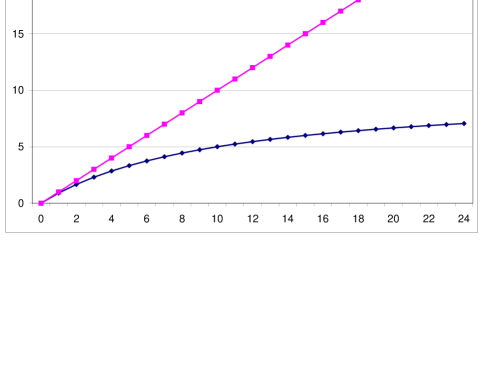
Figure 1: Plot of $\hat{f}$ versus $f$. The transformation of the energy landscape is based on $q=1$ (with $\blacksquare$ on straight line) and $q=2$ (with $\blacklozenge$ below the straight line) for a fixed value of $t=10$.

Figure 2: The energy landscapes of $f$ (with $\blacklozenge$ at top), and for $q=2$, the values of $\hat{f}$ at $t=100$ (with $\blacksquare$, 2nd curve), at $t=10$ (with $\blacktriangle$, 3rd curve) and at $t=1$ (with $\times$ at bottom).

It is worthwhile to note that for values of $q\geq 1$, the rank order of all values of $f$ and $\hat{f}$ are preserved as the following lemma shows.

Lemma 3

For all values of $a>0$ (i.e., $q>1$ and $t>0$) and for all positive reals $x$ and $y$,

$$x>y\Leftrightarrow\frac{x}{1+ax}>\frac{y}{1+ay}.$$

Proof:
For positive $a,x$ and $y,\ x>y$ if and only if $x+axy>y+axy$. Simplifying and dividing each side by $1+ay$ and $1+ax$ (on the right), the result follows.  $\blacksquare$

It is also easy to see from Figure 2 and Lemma 3 that any curve at a given temperature majorizes the corresponding curve at a lower temperature.

The net effect of the energy transformation as indicated in the preceding can be summarized in the following way: it smoothes out the landscape, i.e., reduces the relief of the landscape and lowers the energy values yet preserves the essential relational features of the landscape (in terms of rank order).

5.1 Relating Exponentials and Powerlaws

This energy landscape transformation provides several alternative perspectives on power-law distributions. The flattened landscapes in Figure 2 may explain the heavy tail distributions associated with complex phenomena—the flatter energy landscape makes it easier, in some sense, to move to higher values of $\hat{f}_{i}$ in the energy spectrum. For example, in using the classical Metropolis Algorithm and its associated exponential form using values of $\hat{f}_{i}$, uphill moves are more probable and this leads to a heavy-tailed “steady-state” distribution.

To make this precise, the following theorem shows how this energy transformation in effect parameterizes an exponential distribution and permits it to change into a power-law distribution without the necessity of taking limits. This is the opposite of what Tsallis describes as his “$q$-exponential” (see e.g., [13, p. 537]) where he states a power-law distribution that in the limit becomes exponential (recall that $\lim_{q\rightarrow 1}p_{i}=\pi_{i}$). Thus, in the limit a power-law takes on an exponential form. Here, we use the standard definition of an exponential form which asymptotically becomes a power-law.

Theorem 2

Let $a>0$ and $x$ be such that $ax^{\gamma}>1$ and define

$$\hat{x}=\frac{x^{\gamma}}{1+ax^{\gamma}}$$

for some $\gamma>0$, then for any $\lambda>0$

$$e^{-\lambda\hat{x}}-C_{1}\ \sim\ C_{2}x^{-\gamma}$$ (40)

as $ax\rightarrow\infty$ where the constants $C_{1}=e^{-\lambda/a}$ and $C_{2}=a^{-2}\lambda\,e^{-\lambda/a}$.

Proof:
First note that $\lim_{x\rightarrow\infty}\lambda\hat{x}=\lambda/a$, hence, for any fixed $a>0$ both sides of (40) have limits of 0 as $x\rightarrow\infty$. To show that $e^{-\lambda\hat{x}}-e^{-\lambda/a}$ decreases to zero asymptotically as $1/x^{\gamma}$ (within a constant), first note the identity for any real $x$ and $\gamma>0$,

$$\frac{1}{1+x^{\gamma}}=1-x^{\gamma}+x^{2\gamma}-x^{3\gamma}+x^{4\gamma}-\cdots.$$ (41)

Dividing the numerator and denominator of $\hat{x}$ by $ax^{\gamma}$, we obtain

$$\hat{x}=\frac{x^{\gamma}}{1+ax^{\gamma}}=\frac{1}{a}\left(\frac{1}{1+\frac{1}{ax^{\gamma}}}\right).$$ (42)

Using the general relationship in (41) in the parenthesis in (42) and substituting into $e^{-\lambda\hat{x}}$ yields

$$e^{-\lambda\hat{x}} = \exp\left\{-\frac{\lambda}{a}\left[1-\frac{1}{ax^{\gamma}}+\frac{1}{(ax^{\gamma})^{2}}\cdots\right]\right\}$$ (43)

$$= \exp\left\{-\frac{\lambda}{a}+\frac{\lambda}{a^{2}x^{\gamma}}-\frac{\lambda}{a^{3}x^{2^{\gamma}}}+\cdots\right\}$$

$$= e^{-\lambda/a}\exp\left\{\frac{\lambda}{a^{2}x^{\gamma}}-\frac{\lambda}{a^{3}x^{2^{\gamma}}}+\cdots\right\}.$$

Note that since $\gamma>0$ and $ax^{\gamma}>1$, the series in (43) is absolutely convergent (using the ratio test), hence converges. Substituting a Taylor Series expansion of the exponential in (43) (the second factor) yields

$$e^{-\lambda\hat{x}}=e^{-\lambda/a}\left[1+\left(\frac{\lambda}{a^{2}x^{\gamma}}-\frac{\lambda}{a^{3}x^{2^{\gamma}}}+\cdots\right)+\frac{1}{2}\left(\frac{\lambda^{2}}{a^{4}x^{2\gamma}}+\cdots\right)+\cdots\right]$$ (44)

where we note that the higher order terms of the series in (44) all have powers higher than $a^{4}x^{2\gamma}$ in the denominators (these are not shown). To show that $e^{-\lambda\hat{x}}$ falls off according to a power law, we evaluate the expression

$$\lim_{ax\rightarrow\infty}\frac{\left(e^{-\lambda\hat{x}}-e^{-\lambda/a}\right)}{a^{-2}\lambda\,e^{-\lambda/a}x^{-\gamma}}$$ (45)

to assess its asymptotic behavior and the rate at which it approaches its limiting value (if any). Substituting (44) for the numerator of (45) and multiplying the numerator by $x^{\gamma}$ (from the $x^{-\gamma}$ in the denominator) and reordering the terms of the Taylor Series expansion to indicate only those with powers of $a^{4}x^{2\gamma}$ or less yields

$$x^{\gamma}e^{-\lambda/a}\left[1+\frac{\lambda}{a^{2}x^{\gamma}}-\frac{\lambda}{a^{3}x^{2\gamma}}+\frac{\lambda^{2}}{2a^{4}x^{2\gamma}}\cdots\right]-x^{\gamma}e^{-\lambda/a}$$

$$=\frac{\lambda\,e^{-\lambda/a}}{a^{2}}\left[1-\frac{1}{ax^{\gamma}}+\frac{\lambda}{2a^{2}x^{\gamma}}+\cdots\right]$$

in the numerator. Consequently,

$$\lim_{ax\rightarrow\infty}\frac{x^{\gamma}\left(e^{-\lambda\hat{x}}-e^{-\lambda/a}\right)}{a^{-2}\lambda\,e^{-\lambda/a}}\hskip 20.0pt$$

$$= \lim_{ax\rightarrow\infty}\left[1-\frac{1}{ax^{\gamma}}+\frac{\lambda}{2a^{2}x^{\gamma}}+\cdots\right]$$

$$= \lim_{ax\rightarrow\infty}\left[1-E(a,x)\right]=1$$

where the discrepancy $E(a,x)=\frac{1}{ax^{\gamma}}-\frac{\lambda}{2a^{2}x^{\gamma}}\rightarrow 0$ as $ax\rightarrow\infty$ and hence (40) follows.  $\blacksquare$

Figure 3 compares the decays of $e^{-\lambda\hat{x}}-e^{-\lambda/a}$ and $\lambda\,e^{-\lambda/a}/(a^{2}x^{\gamma})$ for the given values of $a$ and $\lambda$ and shows that the curves are virtually coincident even for the relatively low values of $x$ indicated in the figure.

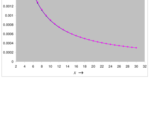
Figure 3: Plots of $e^{-\lambda\hat{x}}-e^{-\lambda/a}$ (the “exponential” series) and $\lambda\,e^{-\lambda/a}a^{-2}x^{-\gamma}$ (the “power law” series) for $a=10,\lambda=\gamma=1$.

5.2 A Recursive Transformation

The form of the $q$–transformation of energy also permits stating an interesting recursive feature that may be useful in relating the level of aggregation to the entropic parameter. Recall that the scale invariant properties indicated in (19) and (25) are based on aggregating energy levels. From these aggregations, several scale-invariant relationships can be defined involving the transformed energy values $\hat{f}_{i}$ defined in (17). But this value is associated with an aggregation of particles, each with its own value of “energy” where this aggregation may actually result from a series of successive aggregations because the $q$–transformation has this recursive aspect. This recursive feature of the energy transformation in (15) is based on the following relationship where we substitute $\hat{f}_{i}$ for $f_{i}$ in (17). This results in

$$\hat{f}_{i,k+1}^{\gamma}=\frac{\hat{f}_{i,k}^{\gamma}}{1+a\hat{f}_{i,k}^{\gamma}}.$$ (46)

For consistency in notation, let $\hat{f}_{i,0}^{\gamma}\equiv f_{i}^{\gamma}$ and it follows that $\hat{f}_{i,1}\equiv\hat{f}_{i}$ for $\gamma=1$ as defined earlier (see (15)). Using these relationships, the following lemma holds.

Lemma 4

The $k^{\mbox{\tiny th}}$ energy transformation $\hat{f}_{i,k}$ raised to any power $\gamma>0$ is related to $f_{i}$ as follows:

$$\hat{f}_{i,k}^{\gamma}=\frac{f_{i}^{\gamma}}{1+k\,af_{i}^{\gamma}}$$ (47)

Proof:
This is an obvious implication of (46) and the use of the induction method.  $\blacksquare$

This suggests there is some equivalence between the number of aggregations and the value of the entropic parameter $q$. That is, the coefficient of $f_{i}$, $ka$, in the denominator of (47) corresponds to a higher value of the entropic parameter. Successive (or larger?) aggregations of energy are, in some sense, equivalent to larger values of $q$. These asymptotic results and the recursion described in Lemma 4 may provide new perspectives on power laws and the nature of critical phenomena which are discussed below.

6 Conclusion and Future Research

This article has explored how various statistical components of a non-extensive system exhibit forms of scale invariance. By aggregating energy levels and defining certain statistical quantities for these aggregated sets in appropriate ways, such as its stationary probability and expected energy levels, various operations on these quantities result in identical mathematical forms as for the corresponding quantities associated with individual energy states provided they are based on a transformed energy value. This energy transformation appears in a number of scale invariant and symmetry relationships.

The manifestation of the energy transformation in these scale invariant forms is a surprising element and bears further investigation. The manner in which it appears suggests that scale invariance exists only by virtue of an energy transformation function. This suggests a view that information (entropy) loss may occur between aggregated states where there has already been some information loss due to prior aggregations. Thus, if one can make the leap from aggregating a system of components to aggregating their associated energy levels, it may provide insight into a number of critical phenomena relating to power-law behaviors. Thus, aggregated system components may further combine to form yet larger aggregations where there is a further loss of entropy due to non-extensivity. But from the recursive property in 4, there is in some sense an equivalence between a succession of aggregations and changes in temperature and/or the entropic parameter $q$. Thus, the level of aggregations in particular parts of a large systems can be seen as equivalent to differences in the temperature, heat capacity and so forth between these different parts of a large system in a far-from-equilibrium regime.

This may also provide some insight into why certain types of systems have particular values of critical exponents. For example, in the border between order and disorder, information loss may occur in connection with how inelastic collisions manifest themselves during a phase transition. But successive aggregations may happen for only a certain fraction of the energy states in a system or the tendency towards aggregation may change with the size of aggregated states. Successive aggregations and the attendant loss of entropy (when $q>1$) may then lead to a certain distribution in terms of the size of these aggregated states indicated by a power-law. The relative frequency of the size of aggregated states and their dependance on macroscopic properties could then explain the particular values of critical exponents as reflecting the average number of aggregations in large systems. In this sense, the universality of these critical exponents suggests that there may be a typical number of successive aggregations with a distribution of this number that reflects and explains the non-integer values of critical exponents.

A number of these issues are further explored and developed in [9] where a generalization of Tsallis’ entropy definition sheds some additional light on these energy transformations. Transformation families are explored as well as recursive relationships similar to those described above. In addition, we use the generalization of Tsallis’ entropy to provide more general ways to state power law distributions in exponential forms, a reverse approach to Tsallis where he provides a mechanism where a power law form can be made asymptotically equal to an exponential form. This also provides clues as to how to take fuller advantage of these results in modeling complex systems and developing simulation models. New approaches for the simulation of complex systems and ways in which to overcome the so-called “broken ergodicity problem” are also explored (see [8]).

Acknowledgements

This research was supported as an Independent Research and Development project at the Johns Hopkins University Applied Physics Laboratory. The author would like to thank Susan Lee, Donna Gregg and William Blackert for their support and encouragement during this project and Drs. Constantino Tsallis, I-Jeng Wang and Alan Weiss for their very useful and helpful suggestions.

References

- [1] I. Andricioaei and J. E. Straub. Generalized simulated annealing algorithms using tsallis statistics: Application to conformational optimization of a tetrapeptide. Physical Review E, 53(4):3055–58, April 1996.
- [2] E. M. F. Curado and C. Tsallis. Generalized statistical mechanics: Connection with thermodynamics. J. of Physics A, 24:L69–L72, 1991. Letters to the Editor.
- [3] M. Fleischer and S.H. Jacobson. Scale invariance properties in the simulated annealing algorithm. Methodology and Computing in Applied Probability, 4:219–241, 2002.
- [4] M. A. Fleischer. Assessing the Performance of the Simulated Annealing Algorithm Using Information Theory. Doctoral dissertation, Case Western Reserve University, Cleveland, Ohio, 1993.
- [5] M. A. Fleischer. Cybernetic optimization by simulated annealing: Accelerating convergence by parallel processing and probabilistic feedback control. Journal of Heuristics, 1(2), 1996.
- [6] M. A. Fleischer. Metaheuristics: Advances and Trends in Local Search Paradigms for Optimization, chapter 28: Generalized Cybernetic Optimization: Solving Continuous Variable Problems, pages 403–418. Kluwer Academic Publishers, 1999.
- [7] M. A. Fleischer and S. H. Jacobson. Metaheuristics: Theory and Applications, chapter Chapter 16: Cybernetic Optimization by Simulated Annealing: An Implementation of Parallel Processing Using Probabilistic Feedback Control. Kluwer Academic Publishers, 1996.
- [8] Mark Fleischer. An extrapolation method for overcoming broken ergodicity in partition function estimation problems using energy transformation functions. 2005. Unpublished manuscript.
- [9] Mark Fleischer. Scale invariance and energy transformations in non-extensive statistical mechanics. 2005. Unpublished manuscript.
- [10] C. Tsallis. Possible generalization of boltzmann-gibbs statistics. Journal of Statistical Physics, 52(1-2):479–487, 1988.
- [11] C. Tsallis, F. Baldovin, R. Cerbino, and P. Pierobon. Introduction to nonextensive statistical mechanics and thermodynamics. In The Physics of Complex Systems: New Advances & Perspectives, Proceedings of the 1953-2003 Jubilee “Enrico Fermi” International Summer School of Physics, 2003.
- [12] C. Tsallis, S. Levy, A. Souza, and R. Maynard. Statistical-mechanical foundation of the ubiquity of lévy distributions in nature. Physical Review Letters, 75(20):3589–93, 1995.
- [13] C. Tsallis, R. S. Mendesc, and A.R. Plastino. The role of constraints within generalized nonextensive statistics. Physica A, 261:534–554, 1998.
- [14] C. Tsallis and D. A. Stariolo. Generalized simulated annealing. Physica A, 233:395–406, 1996.