THE DYNAMICS OF FINANCIAL MARKETS – MANDELBROT’S MULTIFRACTAL CASCADES, AND BEYOND

Abstract

This is a short review in honor of B. Mandelbrot’s 80st birthday, to appear in Wilmott magazine. We discuss how multiplicative cascades and related multifractal ideas might be relevant to model the main statistical features of financial time series, in particular the intermittent, long-memory nature of the volatility. We describe in details the Bacry-Muzy-Delour multifractal random walk. We point out some inadequacies of the current models, in particular concerning time reversal symmetry, and propose an alternative family of multi-timescale models, intermediate between GARCH models and multifractal models, that seem quite promising.

$1$ Evnine-Vaughan Associates, Inc., 456 Montgomery Street, Suite 800, San Francisco, CA 94104, USA
$2$ Science & Finance, Capital Fund Management, 6 Bd Haussmann, 75009 Paris, France
$3$ Service de Physique de l’État Condensé, Centre d’études de Saclay, Orme des Merisiers, 91191 Gif-sur-Yvette Cedex, France
$4$ Laboratoire SPE, CNRS UMR 6134, Université de Corse, 20250 Corte, France
$5$ Consulting in Financial Research, Chemin Charles Baudouin 8, 1228 Saconnex d’Arve, Switzerland

1 Introduction

Financial time series represent an extremely rich and fascinating source of questions, for they store a quantitative trace of human activity, sometimes over hundreds of years. These time series, perhaps surprisingly, turn out to reveal a very rich and particularly non trivial statistical texture, like fat tails and intermittent volatility bursts, have been by now well-characterized by an uncountable number of empirical studies, initiated by Benoit Mandelbrot more than fourty years ago [1]. Quite interestingly, these statistical anomalies are to some degree universal, i.e, common across different assets (stocks, currencies, commodities, etc.), regions (U.S., Europe, Asia) and epochs (from wheat prices in the 18th century to oil prices in 2004). The statistics of price changes is very far from the Bachelier-Black-Scholes random walk model which, nevertheless, is still today the central pillar of mathematical finance: the vast majority of books on option pricing written in the last ten years mostly focus on Brownian motion models and up until recently very few venture into the wonderful world of non Gaussian random walks [2]. This is the world, full of bushes, gems and monsters, that Mandelbrot started exploring for us in the sixties, charting out its scrubby paths, on which droves of scientists – admittedly with some delay – now happily look for fractal butterflies, heavy-tailed marsupials or long-memory elephants. One can only be superlative about his relentless efforts to look at the world with new goggles, and to offer the tools that he forged to so many different communities: mathematicians, physicists, geologists, meteorologists, fractologists, economists – and, for our purpose, financial engineers. In our view, one of Mandelbrot’s most important methodological messages is that one should look at data, charts and graphs in order to build one’s intuition, rather than trust blindly the result of statistical tests, often inadequate and misleading, in particular in the presence of non Gaussian effects [3]. This visual protocol is particularly relevant when modeling financial time series: as discussed below, well chosen graphs often allow one to identify important effects, rule out an idea or construct a model. This might appear as a trivial statement but, as testified by Mandelbrot himself, is not: he fought all his life against the Bourbaki principle that pictures and graphs betray [3]. Unreadable tables of numbers, flooding econometrics papers, perfectly illustrate that figures remain suspicious in many quarters.

The aim of this paper is to give a short review of the stylized facts of financial time series, and of how multifractal stochastic volatility models, inherited from Kolmogorov’s and Mandelbrot’s work in the context of turbulence, fare quite well at reproducing many important statistical features of price changes. We then discuss some inadequacies of the current models, in particular concerning time reversal symmetry, and propose an alternative family of multi-timescale models, intermediate between GARCH models and multifractal models, that seem quite promising. We end on a few words about how these models can be used in practice for volatility filtering and option pricing.

2 Universal features of price changes

The modeling of random fluctuations of asset prices is of obvious importance in finance, with many applications to risk control, derivative pricing and systematic trading. During the last decade, the availability of high frequency time series has promoted intensive statistical studies that lead to invalidate the classic and popular “Brownian walk” model, as anticipated by Mandelbrot [4]. In this section, we briefly review the main statistical properties of asset prices that can be considered as universal, in the sense that they are common across many markets and epochs [5, 6, 7].

If one denotes $p(t)$ the price of an asset at time $t$, the return $r_{\tau}(t)$, at time $t$ and scale $\tau$ is simply the relative variation of the price from $t$ to $t+\tau$: $r_{\tau}(t)=\left[{p(t+\tau)-p(t)}\right]/{p(t)}\simeq\ln p(t+\tau)-\ln p(t)$.

The simplest “universal” feature of financial time series, uncovered by Bachelier in 1900, is the linear growth of the variance of the return fluctuations with time scale. More precisely, if $m\tau$ is the mean return at scale $\tau$, the following property holds to a good approximation:

$$\langle\left(r_{\tau}(t)-m\tau\right)^{2}\rangle_{e}\simeq\sigma^{2}\tau,$$ (1)

where $\langle...\rangle_{e}$ denotes the empirical average. This behaviour typically holds for $\tau$ between a few minutes to a few years, and is equivalent to the statement that relative price changes are, to a good approximation, uncorrelated. Very long time scales (beyond a few years) are difficult to investigate, in particular because the average drift $m$ becomes itself time dependent, but there are systematic effects suggesting some degree of mean-reversion on these long time scales.

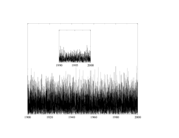
Figure 1: 1-a: Absolute value of the daily price returns for the Dow-Jones index over a century (1900-2000), and zoom on different scales (1990-2000 and 1995). Note that the volatility can remain high for a few years (like in the early 1930’s) or for a few days. This volatility clustering can also be observed on high frequency (intra-day) data. 1-b: Same plot for a Brownian random walk, which shows a featureless pattern in this case.

The volatility $\sigma$ is the simplest quantity that measures the amplitude of return fluctuations and therefore that quantifies the risk associated with some given asset. Linear growth of the variance of the fluctuations with time is typical of the Brownian motion, and, as mentioned above, was proposed as a model of market fluctuations by Bachelier. In this model, returns are not only uncorrelated, as mentioned above, but actually independent and identical Gaussian random variables. However, this model completely fails to capture other statistical features of financial markets that even a rough analysis of empirical data allows one to identify, at least qualitatively:

• The distribution of returns is in fact strongly non Gaussian and its shape continuously depends on the return period $\tau$: for $\tau$ large enough (around few months), one observes quasi-Gaussian distributions while for small $\tau$ values, the return distributions have a strong kurtosis (see Fig. 2). Several careful studies suggest that these distributions can be characterized by Pareto (power-law) tails $|r|^{-1-\mu}$ with an exponent $\mu$ in the range $3-5$ even for liquid markets such as the US stock index, major currencies, or interest rates [8, 9, 5, 10]. Note that $\mu>2$, and excludes an early suggestion by Mandelbrot that security prices could be described by Lévy stable laws. Emerging markets, however, have even more extreme tails, with an exponent $\mu$ that can be less than $2$ – in which case the volatility is formally infinite – as found by Mandelbrot in his famous study of cotton prices [4]. A natural conjecture is that as markets become more liquid, the value of $\mu$ tends to increase (although illiquid, yet very regulated markets, could on the contrary show truncated tails because of artificial trading rules [11]).

• Another striking feature is the intermittent and correlated nature of return amplitudes. At some given time period $\tau$, the volatility is a quantity that can be defined locally in various ways: the simplest ones being the square return $r^{2}_{\tau}(t)$ or the absolute return $|r_{\tau}(t)|$, or a local moving average of these quantities. The volatility signals are characterized by self-similar outbursts (see Fig. 1) that are similar to intermittent variations of dissipation rate in fully developed turbulence [12]. The occurrence of such bursts are strongly correlated and high volatility periods tend to persist in time. This feature is known as volatility clustering [13, 14, 6, 7]. This effect can analyzed more quantitatively: the temporal correlation function of the (e.g. daily) volatility can be fitted by an inverse power of the lag, with a rather small exponent in the range $0.1-0.3$ [14, 15, 16, 7, 17].

• One observes a non-trivial “multifractal” scaling [18, 19, 20, 21, 17, 22, 23], in the sense that higher moments of price changes scale anomalously with time:

  $$M_{q}(\tau)=\langle\left|r_{\tau}(t)-m\tau\right|^{q}\rangle_{e}\simeq A_{q}\tau^{\zeta_{q}},$$ (2)

  where the index $\zeta_{q}$ is not equal to the Brownian walk value $q/2$. As will be discussed more precisely below, this behaviour is intimately related to the intermittent nature of the volatility process.

• Past price changes and future volatilities are negatively correlated, at least on stock markets. This is the so called leverage effect, which reflects the fact that markets become more active after a price drop, and tend to calm down when the price rises. This correlation is most visible on stock indices [24]. This leverage effect leads to an anomalous negative skew in the distribution of price changes as a function of time.

The most important message of these empirical studies is that price changes behave very differently from the simple geometric Brownian motion: extreme events are much more probable, and interesting non linear correlations (volatility-volatility and price-volatility) are observed. These “statistical anomalies” are very important for a reliable estimation of financial risk and for quantitative option pricing and hedging, for which one often requires an accurate model that captures return statistical features on different time horizons $\tau$. It is rather amazing to remark that empirical properties (i-iv) are, to some extent, also observed on experimental velocity data in fully developed turbulent flows (see Fig. 2). The framework of scaling theory and multifractal analysis, initially proposed to characterize turbulent signals by Mandelbrot and others [12], may therefore be well-suited to further characterize statistical properties of price changes on different time periods.

Figure 2: Continuous deformation of turbulent velocity increments and financial returns distributions from small (top) to large (bottom) scales. 2-a: Standardized probability distribution functions of spatial velocity increments at different length scales in a high Reynolds number wind tunnel turbulence experiment. The distributions are plotted in logarithmic scale so that a parabola corresponds to a Gaussian distribution. 2-b: Standardized p.d.f. of S&P 500 index returns at different time scales from few minutes to one month. Notice that because of sample size limitation, the noise amplitude is larger than in turbulence.

3 From multifractal scaling to cascade processes

3.1 Multi-scaling of asset returns

For the geometric Brownian motion, or for the Lévy stable processes first suggested by Mandelbrot as an alternative, the return distribution is identical (up to a rescaling) for all $\tau$. As emphasized in previous section, the distribution of real returns is not scale invariant, but rather exhibits multi-scaling. Fig. 3 illustrates the empirical multifractal analysis of S&P 500 index return. As one can see in Fig. 3(b), the scaling behavior (2) that corresponds to a linear dependence in a log-log representation of the absolute moments versus the time scale $\tau$, is well verified over some range of time scales (typically 3 decades).

Figure 3: Multifractal scaling analysis of S&P 500 returns. 3-a: S&P 500 index price series sampled at a 5 minutes rate. 3-b: First five absolute moments of the index (defined in Eq. (2)) as a function of the time period $\tau$ in double logarithmic representation. For each moment, a linear fit of the small scale behavior provides an estimate of $\zeta_{q}$. 3-c: Moment ratios $M_{q}(\tau)/M_{2}(\tau)^{q/2}$ in log-log representation. Such curves would be flat for a geometric Brownian process. 3-d: $\zeta_{q}$ spectrum estimate versus $q$. Negative $q$ values are obtained using a wavelet method as defined in e.g. [28]. This function is well fitted by a Kolmogorov log-normal spectrum (see text).

The multifractal nature of the index fluctuations can directly be checked in Fig. 3(c), where one sees that the moment ratios strongly depend on the scale $\tau$. The estimated $\zeta_{q}$ spectrum (Fig. 3(d)) has a concave shape that is well fitted by the parabola: $\zeta_{q}=q(1/2+\lambda^{2})-\lambda^{2}q^{2}/2$ with $\lambda^{2}\simeq 0.03$. The coefficient $\lambda^{2}$ that quantifies the curvature of the $\zeta_{q}$ function is called, in the framework of turbulence theory, the intermittency coefficient. The most natural way to account for the multi-scaling property (2) is through the notion of cascade from coarse to fine scales.

3.2 The cascade picture

As noted previously, for the geometric Brownian motion, the return probability distributions at different time periods $\tau$ are Gaussian and thus differ only by their width that is proportional to $\sqrt{\tau}$. If $x(t)$ is a Brownian motion, this property can be shortly written as

$$r_{\tau}(t) \operatornamewithlimits{=}_{law} \sigma_{\tau}\varepsilon(t)$$ (3)

$$\sigma_{s\tau} = s^{1/2}\sigma_{\tau}$$ (4)

where $\operatornamewithlimits{=}_{law}$ means that the two quantities have the same probability distribution, $\varepsilon(t)$ is a standardized Gaussian white noise and $\sigma_{\tau}$ is the volatility at scale $\tau$. When going from some scale $\tau$ to the scale $s\tau$, the return volatility is simply multiplied by $s^{1/2}$. The cascade model assumes such a multiplicative rule but the multiplicative factor is now a random variable and the volatility itself becomes a random process $\sigma_{\tau}(t)$:

$$r_{\tau}(t) \operatornamewithlimits{=}_{law} \sigma_{\tau}(t)\varepsilon(t)$$ (5)

$$\sigma_{s\tau}(t) \operatornamewithlimits{=}_{law} W_{s}\sigma_{\tau}(t)$$ (6)

where the law of $W_{s}$ depends only on the scale ratio $s$ and is independent of $\sigma_{\tau}(t)$. Let $T$ be some coarse time period and let $s<1$. Then, by setting $W=e^{\xi}$, and by iterating equation (6) $n$ times, one obtains:

$$\sigma_{s^{n}T}(t)\operatornamewithlimits{=}_{law}W_{s^{n}}\sigma_{T}(t)\operatornamewithlimits{=}_{law}e^{\sum_{\ell=1}^{n}\xi_{\ell,s}}\sigma_{T}(t)$$ (7)

Therefore, the logarithm of the volatility at some fixed scale $\tau=s^{n}T$, can be written as a sum of an arbitrarily large number $n$ of independent, identically distributed random variables. Mathematically, this means that the logarithm of the volatility (and hence $\xi$, the logarithm of the “weights” $W$) belongs the the class of the so-called infinitely divisible distributions [25]. The simplest of such distributions (often invoked using the central limit theorem) is the Gaussian law. In that case, the volatility is a log-normal random variable. As explained in the next subsection, this is precisely the model introduced by Kolmogorov in 1962 to account for the intermittency of turbulence [26]. It can be proven that the random cascade equations (5) and (6) directly lead to the deformation of return probability distribution functions as observed in Fig. 2. Using the fact that $\xi_{s}$ is a Gaussian variable of mean $\mu\ln(s)$ and variance $\lambda^{2}\ln(s)$, one can compute the absolute moment of order $q$ of the returns at scale $\tau=s^{n}T$ ($s<1$). One finds:

$$\langle|r_{\tau}(t)|^{q}\rangle=A_{q}\left(\frac{\tau}{T}\right)^{\mu q-\lambda^{2}q^{2}/2}$$ (8)

where $A_{q}=\langle|r_{T}(t)|^{q}\rangle$.

Using a simple multiplicative cascade, we thus have recovered the empirical findings of previous sections. For log-normal random weights $W_{s}$, the return process is multifractal with a parabolic $\zeta_{q}$ scaling spectrum: $\zeta_{q}=q\mu-\lambda^{2}q^{2}/2$ where the parameter $\mu$ is related to the mean of $\ln W_{s}$ and the curvature $\lambda^{2}$ (the intermittency coefficient) is related to the variance of $\ln W_{s}$ and therefore to the variance of the log-volatility $\ln(\sigma_{\tau})$:

$$\langle(\ln\sigma_{\tau}(t))^{2}\rangle-\langle\ln\sigma_{\tau}(t)\rangle^{2}=-\lambda^{2}\ln(\tau)+V_{0}$$ (9)

The random character of $\ln W_{s}$ is therefore directly related to the intermittency of the returns.

4 The multifractal random walk

The above cascade picture assumes that the volatility can be constructed as a product of random variables associated with different time scales. In the previous section, we exclusively focused on return probability distribution functions (mono-variate laws) and scaling laws associated with such models. Explicit constructions of stochastic processes which marginals satisfy a random multiplicative rule, were first introduced by Mandelbrot [27] and are known as Mandelbrot’s cascades or random multiplicative cascades. The construction of a Mandelbrot cascade, illustrated in Fig. 4, always involves a discrete scale ratio $s$ (generally $s=1/2$). One begins with the volatility at the coarsest scale and proceeds in a recursive manner to finer resolutions: The $n$-th step of the volatility construction corresponds to scale $2^{-n}$ and is obtained from the $(n-1)$-th step by multiplication with a positive random process $W$ the law of which does not depend on $n$. More precisely, the volatility in each subinterval is the volatility of its parent interval multiplied by an independent copy of $W$.

Mandelbrot cascades are considered to be the paradigm of multifractal processes and have been extensively used for modeling scale-invariance properties in many fields, in particular statistical finance by Mandelbrot himself [19, 22]. However, this class of models presents several drawbacks: (i) they involve a preferred scale ratio $s$, (ii) they are not stationary and (iii) they violate causality. In that respect, it is difficult to see how such models could arise from a realistic (agent based) description of financial markets.

Recently, Bacry, Muzy and Delour (BMD) [17, 29] introduced a model that does not possess any of the above limitations and captures the essence of cascades through their correlation structure (see also [31, 32] for alternative multifractal models).

Figure 4: Multiplicative construction of a Mandelbrot cascade. One starts at the coarsest scale $T$ and constructs the volatility fluctuations at fine scales using a recursive multiplication rule. The variables $W$ are independent copies of the same random variable.

In the BMD model, the key ingredient is the volatility correlation shape that mimics cascade features. Indeed, as remarked in ref. [33], the tree like structure underlying a Mandelbrot cascade, implies that the volatility logarithm covariance decreases very slowly, as a logarithm function, i.e.,

$$\left\langle\ln(\sigma_{\tau}(t))\ln(\sigma_{\tau}(t+\Delta t))\right\rangle-\left\langle\ln(\sigma_{\tau}(t))\right\rangle^{2}=C_{0}-\lambda^{2}\ln(\Delta t+\tau)$$ (10)

This equation can be seen as a generalization of Kolmogorov equation (9) that describes only the behavior of the log-volatility variance. It is important to note that such a logarithmic behaviour of the covariance has indeed been observed for empirically estimated log-volatilities in various stock market data [33]. The BMD model involves Eq. (10) within the continuous time limit of a discrete stochastic volatility model. One first discretizes time in units of an elementary time step $\tau_{0}$ and sets $t\equiv i\tau_{0}$. The volatility $\sigma_{i}$ at “time” $i$ is a log-normal random variable such that $\sigma_{i}=\sigma_{0}\exp\xi_{i}$, where the Gaussian process $\xi_{i}$ has the same covariance as in Eq. (10):

$$\langle{\xi_{i}}\rangle=-\lambda^{2}\ln(\frac{T}{\tau_{0}})\equiv\mu_{0};\qquad\langle{\xi_{i}\xi_{j}}\rangle-\mu_{0}^{2}=\lambda^{2}\ln(\frac{T}{\tau_{0}})-\lambda^{2}\ln(|i-j|+1),$$ (11)

for $|i-j|\tau_{0}\leq T$. Here $T$ is a large cut-off time scale beyond which the volatility correlation vanishes. In the above equation, the brackets stands for the mathematical expectation. The choice of the mean value $\mu_{0}$ is such that $\langle{\sigma^{2}}\rangle=\sigma_{0}^{2}$. As before, the parameter $\lambda^{2}$ measures the intensity of volatility fluctuations (or, in the finance parlance, the ‘vol of the vol’), and corresponds to the intermittency parameter.

Figure 5: Multifractal properties of BMD model. 5-a: Exponential of a BMD process realization. The parameters have been adjusted in order to mimic the features of S&P 500 index reported in Fig. 3. 5-b: Multifractal scaling of BMD return moments for $q=1,2,3,4,5$. 5-c: Estimated $\zeta_{q}$ spectrum ($\circ$) compared with the log-normal analytical expression (solid line). 5-d: Evolution of the return probability distributions across scales, from nearly Gaussian at coarse scale (bottom) to fat tailed law at small scales (top). (e) Log-volatility covariance as a function of the logarithm of the lag $\tau$.

Now, the price returns are constructed as:

$$x\left[(i+1)\tau_{0}\right]-x\left[i\tau_{0}\right]=r_{\tau_{0}}(i)\equiv\sigma_{i}\varepsilon_{i}=\sigma_{0}e^{\xi_{i}}\varepsilon_{i},$$ (12)

where the $\varepsilon_{i}$ are a set of independent, identically distributed random variables of zero mean and variance equal to $\tau_{0}$. One also assumes that the $\varepsilon_{i}$ and the $\xi_{i}$ are independent (but see [34] where some correlations are introduced). In the original BMD model, $\varepsilon_{i}$’s are Gaussian, and the continuous time limit $\tau_{0}={\rm dt}\to 0$ is taken. Since $x=\ln p$, where $p$ is the price, the exponential of a sample path of the BMD model is plotted in Fig. 5(a), which can be compared to the real price chart of 2(a).

The multifractal scaling properties of this model can be computed explicitly. Moreover, using the properties of multivariate Gaussian variables, one can get closed expressions for all even moments $M_{q}(\tau)$ ($q=2k$). In the case $q=2$ one trivially finds:

$$M_{2}(\tau=\ell\tau_{0})=\sigma_{0}^{2}\,\ell\tau_{0}\equiv\sigma_{0}^{2}\tau,$$ (13)

independently of $\lambda^{2}$. For $q\neq 2$, one has to distinguish between the cases $q\lambda^{2}<1$ and $q\lambda^{2}>1$. For $q\lambda^{2}<1$, the corresponding moments are finite, and one finds, in the scaling region $\tau_{0}\ll\tau\leq T$, a genuine multifractal behaviour [17, 29], for which Eq.  (2) holds exactly. For $q\lambda^{2}>1$, on the other hand, the moments diverge, suggesting that the unconditional distribution of $x(t+\tau)-x(t)$ has power-law tails with an exponent $\mu=1/\lambda^{2}$ (possibly multiplied by some slow function). These multifractal scaling properties of BMD processes are numerically checked in Figs. 5-a and 5-b where one recovers the same features as in Fig. 3 for the S&P 500 index. Since volatility correlations are absent for $\tau\gg T$, the scaling becomes that of a standard random walk, for which $\zeta_{q}=q/2$. The corresponding distribution of price returns thus becomes progressively Gaussian. An illustration of the progressive deformation of the distributions as $\tau$ increases, in the BMD model is reported in Fig. 5-c. This figure can be directly compared to Fig. 2. As shown in Fig. 5-e, this model also reproduces the empirically observed logarithmic covariance of log-volatility (Eq. (10). This functional form, introduced at a “microscopic” level (at scale $\tau_{0}\to 0$), is therefore stable across finite time scales $\tau$.

To summarize, the BMD process is attractive for modeling financial time series since it reproduces most “stylized facts” reviewed in section 2 and has exact multifractal properties as described in section 3. Moreover, this model has stationary increments, does not exhibit any particular scale ratio and can be formulated in a purely causal way: the log volatility $\xi_{i}$ can be expressed as a sum over “past” random shocks, with a memory kernel that decays as the inverse square root of the time lag [35]. Let us mention that generalized stationary continuous cascades with compound Poisson and infinitely divisible statistics have been recently contructed and mathematically studied by Mandelbrot and Barral [36], and in [30] However, there is no distinction between past and future in this model – but see below.

5 Multifractal models: empirical data under closer scrutiny

Multifractal models either postulate or predict a number of precise statistical features that can be compared with empirical price series. We review here several successes, but also some failures of this family of models, that suggest that the century old quest for a faithful model of financial prices might not be over yet, despite Mandelbrot’s remarkable efforts and insights. Our last section will be devoted to an idea that may possibly bring us a little closer to the yet unknown “final” model.

5.1 Volatility distribution

Mandelbrot’s cascades construct the local volatility as a product of random volatilities over different scales. As mentioned above, this therefore leads to the local volatility being log-normally distributed (or log infinitely divisible), an assumption that the BMD model postulates from scratch. Several direct studies of the distribution of the volatility are indeed compatible with log-normality; option traders actually often think of volatility changes in relative terms, suggesting that the log-volatility is the natural variable. However, other distributions, such as an inverse gamma distribution fits the data equally well, or even better [37, 7].

5.2 Intermittency coefficient

One of the predictions of the BMD model is the equality between the intermittency coefficient estimated from the curvature of the $\zeta_{q}$ function and the slope of the log-volatility covariance logarithmic decrease. The direct study of various empirical log-volatility correlation functions, show that can they can indeed be fitted by a logarithm of the time lag, with a slope that is in the same ball-park as the corresponding intermittency coefficient $\lambda^{2}$. The agreement is not perfect, though. These empirical studies furthermore suggest that the integral time $T$ is on the scale of a few years [17].

5.3 Tail index

As mentioned above, and as realized by Mandelbrot long ago through his famous “star equation” [27], multifractal models lead to power law tails for the distribution of returns. The BMD model predicts that the power-law index should be $\mu=1/\lambda^{2}$, which, for the empirical values of $\lambda^{2}\sim 0.03$, leads to a value of $\mu$ ten times larger than the empirical value of $\mu$, found in the range $3-5$ for many assets [8, 9, 5]. Of course, the random variable $\varepsilon$ could itself be non Gaussian and further fattens the tails. However, as recently realized by Bacry, Kozhemyak and Muzy [38], a kind of ‘ergodicity breaking’ seems to take place in these models, in such a way that the theoretical value $\mu=1/\lambda^{2}$ may not correspond to the most probable value of the estimator of the tail of the return distribution for a given realization of the volatility, the latter being much smaller than the former. So, even if this scenario is quite non trivial, multifractal models with Gaussian residuals may still be consistent with fat tails.

5.4 Time reversal invariance

Both Mandelbrot’s cascade models and the BMD model are invariant under time reversal symmetry, meaning that no statistical test of any nature can distinguish between a time series generated with such models and its time reversed. There are however various direct indications that real price changes are not time reversal invariant. One well known fact is the “leverage effect” (point (iv) of Section 2, see also [24]), whereby a negative price change is on average followed by a volatility increase. This effect leads to a skewed distribution of returns, which in turn can be read as a skew in option volatility smiles. In the BMD model, one has by symmetry that all odd moments of the process vanish. A simple possibility, recently investigated in [34], is to correlate negatively the variable $\xi_{i}$ with ‘past’ values of the variables $\varepsilon_{j}$, $j<i$, through a kernel that decays as a power-law. In this case, the multifractality properties of the model are preserved, but the expression for $\zeta_{q}$ is different for $q$ even and for $q$ odd (see also [39]).

Another effect breaking the time reversal invariance is the asymmetric structure of the correlations between the past and future volatilities at different time horizons. This asymmetry is present in all time series, even when the above leverage effect is very small or inexistent, such as for the exchange rate between two similar currencies (e.g. Dollar vs. Euro). The full structure of the volatility correlations is shown by the following “mug shots” introduced in [40]. These plots show how past volatilities measured on different time horizons (horizontal axis) affect future volatilities, again on different time horizons (vertical axis). For empirical price changes, the correlations between past volatilities and future volatilities is asymmetric, as shown on Fig. 6. This figure reveals clearly two very important features: (a) the volatility at a given time horizon is affected mainly by the volatilities at longer time horizon (the “cascade” effect, partly discovered in [33]), and (b) correlations are strongest for time horizons corresponding to the natural human cycles, i.e: intra-day, one day, one week and one month. The feature (a) points to a difference with the volatility cascade used in turbulence, where eddies at a given scale break down into eddies at the immediately smaller scale. For financial time series, the volatilities at all time horizons feed the volatility at the shortest time horizon [40]. The overall asymmetry around the diagonal of the figure measures the asymmetry of the price time series under time reversal invariance. For a time reversal symmetric process, these mug shots are symmetric. An example of a very symmetric process is given in Fig. 7, for a volatility cascade as given in Eq. (7). The process for the “log-volatility” $\xi_{n}$ at the $n$-th scale obeys an Ornstein-Uhlenbeck process, with a characteristic time $s^{-n}$. In order to obtain a realistic cascade of volatilities, the (instantaneous) mean for the process $\xi_{n}$ is taken as the volatility at the larger scale $\xi_{n-1}$. Yet, the resulting mug shot is very different from the empirical one, in particular it is exactly symmetric (at least theoretically).

Building a multifractal model that reproduces the observed time asymmetry is still an open problem. There might however be other avenues, as we now discuss.

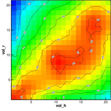
Figure 6: The correlation between past historical volatilities $\sigma_{h}[\tau]$ ($\ln(\tau)$ on the horizontal axis) and the future realized volatilities $\sigma_{r}[\tau^{\prime}]$ ($\ln(\tau^{\prime})$ on the vertical axis) for the USD/CHF foreign exchange time series. The units correspond to the time intervals: 1h 12min for (1), 4h 48min (4), 1d 14h 24min (10), 6d 9h 36min (14), and 25d 14h 24min (18).

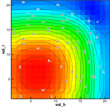
Figure 7: As for Fig. 6, but for a theoretical volatility cascade with Ornstein-Uhlenbeck partial log-volatilities $\xi_{n}$. The cascade includes components from 0.25 day to 4 days. Note the symmetry of this mug-shot, to be contrasted with the previous figure. A similar, symmetric mug-shot would also obtain for multifractal models..

6 Multi-timescale GARCH processes and statistical feedback

The above description of financial data using multifractal, cascade-like ideas is still mostly phenomenological. An important theoretical issue is to understand the underlying mechanisms that may give rise to the remarkable statistical structure of the volatility emphasized by multifractal models: (nearly) log-normal, with logarithmically decaying correlations. Furthermore, from a fundamental point of view, the existence of two independent statistical processes, one for returns and another for the volatility, may not be very natural. In stochastic volatility models, such as the multifractal model, the volatility has its own dynamics and sources of randomness, without any feedback from the price behaviour. The time asymmetry revealed by the above mug-shots however unambiguously shows that a strong feedback, beyond the leverage effect, exists in financial markets.

This time asymmetry, on the other hand, is naturally present in GARCH models, where the volatility is a (deterministic) function of the past price changes. The underlying intuition is that when recent price changes are large, the activity of market agents increases, in turn creating possibly large price changes. This creates a non linear feedback, where rare events trigger more rare events, generating non trivial probability distributions and correlations. Most GARCH models describe the feedback as quadratic in past returns, with the following general form. The (normalized) return at time $i$, computed over a time interval $k\tau_{0}$ is given by $\tilde{r}_{i,k}=(x_{i}-x_{i-k})/\sqrt{k\tau_{0}}$. The general form of the volatility is:

$$\sigma_{i}^{2}=\sigma_{0}^{2}+\sum_{j<i}\sum_{k>0}L(i-j;k)\tilde{r}_{j,k}^{2}$$ (14)

where $\sigma_{0}$ is a ‘bare’ volatility that would prevail in the absence of feedback, and $L(i-j;k)$ a kernel that describes how square returns on different time scales $k$, computed for different days $j$ in the past, affect the uncertainty of the market at time $i$. [Usually, these processes are rather formulated through a set of recursive equations, with a few parameters. By expanding these recursion equations, one obtains the $AR(\infty)$ form given above.]

The literature on GARCH-like processes is huge, with literaly dozen of variations that have been proposed (for a short perspective, see [40, 41]). Some of these models are very successful at reproducing most of the empirical facts, including the “mug shot” for the volatility correlation. An example, that was first investigated in [40] and recently rediscovered in [42] as a generalization of previous work [43], is to choose $L(i-j;k)\equiv\delta_{i,j}K(k)$. This choice means that the current volatility is only affected by observed price variations between different dates $i-k$ in the past and today $i$. The quadratic dependence of the volatility on past returns is precisely the one found in the framework of the statistical feedback process introduced in [43], where the volatility is proportional to a negative power of the probability of past price changes – hence the increased volatility after rare events. The time series resulting from the above choice of kernel are found to exhibit fat, power-law tails, volatility bursts and long range memory [42]. Furthermore, the distribution of volatilities is found to be very close to log-normal [42]. Choosing $K$ to be a power-law of time [40, 44] allows one to reproduce the power-law decay of volatility correlations observed in real data [14, 16, 7, 17], the power-law response of the volatility to external shocks [35, 45], an apparent multifractal scaling [46] and, most importantly for our purpose, the shape of the mug-shots shown above [40]. Many of these results can be obtained analytically [42, 44]. Note that one could choose $K(k)$ to spike for the day, week, month time scales unveiled by the mug-shots [40, 41]. Yet, a detailed systematic comparison of empirical facts against the predictions of the models, GARCH-like or multifractal-like, is still lacking.

The above model can be generalized further by postulating a Landau-like expansion of the volatility as a function of past returns as:

$$\sigma_{i}^{2}=\sigma_{0}^{2}+\sum_{k>0}K(k)G[\tilde{r}_{i,k}]$$ (15)

with $G(r)=g_{1}r+g_{2}r^{2}+...$ [44]. The case $g_{1}=0$ corresponds to the model discussed above, whereas $g_{1}<0$ allows one to reproduce the leverage effect and a negative skewness. Other effects, such as trends, could also be included [47]. The interest of this type of models, compared to multifractal stochastic volatility models, is that their fundamental justification, in terms of agent based strategy, is relatively direct and plausible. One can indeed argue that agents use thresholds for their interventions (typically stop losses, entry points or exit points) that depend on the actual path of the price over some investment horizon, which may differ widely between different investors – hence a power-law like behaviour of the kernels $K(k)$. Note in passing that, quite interestingly, Eq. (14) is rather at odds with the efficient market hypothesis, which asserts that the price past history should have no bearing whatsoever on the behaviour of investors. Establishing the validity of Eq. (14) could have important repercussions on that front, too.

7 Conclusion: why are these models useful anyway ?

For many applications, such as risk control and option pricing, we need a model that allows one to predict, as well as possible, the future volatility of an asset over a certain time horizon, or even better, to predict that probability distribution of all possible price paths between now and a certain future date. A useful model should therefore provide a well defined procedure to filter the series past price changes, and to compute the weights of the different future paths. Multifractal models offer a well defined set of answers to these questions, and their predictive power have been shown to be quite good [31, 48, 32]. Other models, more in the spirit of GARCH or of Eq. (15) have been shown to also fare rather well [49, 41, 44, 47]. Filtering past information within both frameworks is actually quite similar; it would be interesting to compare their predictive power in more details, with special care for non-Gaussian effects. Once calibrated, these models can in principle be used for VaR estimates and option pricing. However, their mathematical complexity do not allow for explicit analytical solutions (except in some special cases, see e.g. [43]) and one has to resort to numerical, Monte-Carlo methods. The difficulty for stochastic volatility models or GARCH models in general is that the option price must be computed conditional to the past history [50], which considerably complexifies Monte-Carlo methods, in particular for path dependent options, or when non-quadratic hedging objectives are considered. In other words, both the option price and the optimal hedge are no longer simple functions of the current price, but functionals of the whole price history. Finding operational ways to generalize, e.g. the method of Longstaff and Schwartz [51], or the optimally hedged Monte-Carlo method of [52] to account for this history dependence, seems to us a major challenge if one is to extract the best of these sophisticated volatility models. The toolkit that Mandelbrot gave us to describe power-law tails and long-range memory is still incomplete: is there an Ito lemma to deal elegantly with multifractal phenomena? Probably not – but as Paul Cootner pointed out long ago in his review of the famous cotton price paper [4], Mandelbrot promised us with blood, sweat, toil and tears. After all, a faithful model, albeit difficult to work with, is certainly better than Black and Scholes’s pristine, but often misleading, simplicity [53].

References

- [1] For an inspiring recent account, see B. B. Mandelbrot, R. Hudson, The (mis)behaviour of markets, Perseus Books, Cambridge MA (2004)
- [2] E. Montroll, M. Shlesinger, The wonderful world of random walks, in Non Equilibrium Phenomena II, Studies in Statistical Mechanics, 11, E. Montroll, J. Lebowitz Edts, North Holland (1984).
- [3] see, e.g. [1], p. 88 and sq.
- [4] B. B. Mandelbrot, The variation of certain speculative prices, J. Business 36, 394 (1963).
- [5] D. M. Guillaume, M. M. Dacorogna, R. D. Davé, U. A. Müller, R. B. Olsen and O. V. Pictet, Finance and Stochastics 1 95 (1997); M. Dacorogna, R. Gençay, U. Müller, R. Olsen, and O. Pictet, An Introduction to High-Frequency Finance (Academic Press, London, 2001).
- [6] R. Mantegna & H. E. Stanley, An Introduction to Econophysics, Cambridge University Press, 1999.
- [7] J.-P. Bouchaud and M. Potters, Theory of Financial Risks and Derivative Pricing, Cambridge University Press, 2004.
- [8] V. Plerou, P. Gopikrishnan, L.A. Amaral, M. Meyer, H.E. Stanley, Scaling of the distribution of price fluctuations of individual companies, Phys. Rev. E60 6519 (1999); P. Gopikrishnan, V. Plerou, L. A. Amaral, M. Meyer, H. E. Stanley, Scaling of the distribution of fluctuations of financial market indices, Phys. Rev. E 60 5305 (1999)
- [9] T. Lux, The stable Paretian hypothesis and the frequency of large returns: an examination of major German stocks, Applied Financial Economics, 6, 463, (1996).
- [10] F. Longin, The asymptotic distribution of extreme stock market returns, Journal of Business, 69 383 (1996)
- [11] K. Matia, M. Pal, H. E. Stanley, H. Salunkay, Scale dependent price fluctuations for the Indian stock market, cond-mat/0308013.
- [12] U. Frisch, Turbulence: The Legacy of A. Kolmogorov, Cambridge University Press (1997).
- [13] A. Lo, Long term memory in stock market prices, Econometrica, 59, 1279 (1991).
- [14] Z. Ding, C. W. J. Granger and R. F. Engle, A long memory property of stock market returns and a new model, J. Empirical Finance 1, 83 (1993).
- [15] M. Potters, R. Cont, J.-P. Bouchaud, Financial Markets as Adaptive Ecosystems, Europhys. Lett. 41, 239 (1998).
- [16] Y. Liu, P. Cizeau, M. Meyer, C.-K. Peng, H. E. Stanley, Correlations in Economic Time Series, Physica A245 437 (1997)
- [17] J.-F. Muzy, J. Delour, E. Bacry, Modelling fluctuations of financial time series: from cascade process to stochastic volatility model, Eur. Phys. J. B 17, 537-548 (2000).
- [18] S. Ghashghaie, W. Breymann,J. Peinke, P. Talkner, Y. Dodge, Turbulent cascades in foreign exchange markets Nature 381 767 (1996).
- [19] B. B. Mandelbrot, Fractals and Scaling in Finance, Springer, New York, 1997; A. Fisher, L. Calvet, B.B. Mandelbrot, Multifractality of DEM/$ rates, Cowles Foundation Discussion Paper 1165 (1997); B.B. Mandelbrot, A multifractal walk down Wall street, Scientific American, Feb. (1999).
- [20] F. Schmitt, D. Schertzer, S. Lovejoy, Multifractal analysis of Foreign exchange data, Applied Stochastic Models and Data Analysis, 15 29 (1999);
- [21] M.-E. Brachet, E. Taflin, J.M. Tchéou, Scaling transformation and probability distributions for financial time series, e-print cond-mat/9905169
- [22] T. Lux, Turbulence in financial markets: the surprising explanatory power of simple cascade models, Quantitative Finance 1, 632, (2001 )
- [23] L. Calvet, A. Fisher, Multifractality in asset returns, theory and evidence, The Review of Economics and Statistics, 84, 381 (2002)
- [24] J.P. Bouchaud, A. Matacz, M. Potters, The leverage effect in financial markets: retarded volatility and market panic Physical Review Letters, 87, 228701 (2001)
- [25] W. Feller, An introduction to probability theory and is applications, Vol. 2, John Wiley & Sons (1971).
- [26] A.N. Kolmogorov, A refinement of previous hypotheses concerning the local structure of turbulence in a viscous incompressible fluid at high Reynolds number, J. Fluid. Mech. 13, 82 (1962).
- [27] B.B. Mandelbrot, Intermittent turbulence in self-similar cascades: divergence of high moments and dimension of the carrier, J. Fluid Mech. 62, 331 (1974).
- [28] J.F. Muzy, E. Bacry and A. Arneodo, The multifractal formalism revisited with wavelets, Int. J. of Bifurcat. and Chaos 4, 245 (1994)
- [29] E. Bacry, J. Delour and J.F. Muzy, Multifractal random walk, Phys. Rev. E 64, 026103 (2001).
- [30] J.F. Muzy and E. Bacry, Multifractal stationary random measures and multifractal random walks with log-infinitely divisible scaling laws, Phys. Rev. E 66, 056121 (2002).
- [31] L. Calvet, A. Fisher, Forecasting multifractal volatility, Journal of Econometrics, 105, 27, (2001), L. Calvet, A. Fisher, How to Forecast Long-Run Volatility: Regime Switching and the Estimation of Multifractal Processes, J. Financial Econometrics, 2, 49 (2004).
- [32] T. Lux, Multi-Fractal Processes as a Model for Financial Returns: Simple Moment and GMM Estimation, in revision for Journal of Business and Economic Statistics.
- [33] A. Arneodo, J.-F. Muzy, D. Sornette, Causal cascade in the stock market from the ‘infrared’ to the ‘ultraviolet’, Eur. Phys. J. B 2, 277 (1998)
- [34] B. Pochart and J.P. Bouchaud, The skewed multifractal random walk with applications to option smiles, Quantitative Finance, 2, 303 (2002).
- [35] D. Sornette, Y. Malevergne, J.F. Muzy, What causes crashes, Risk Magazine, 67 (Feb. 2003).
- [36] B. B. Mandelbrot, J. Barral, Multifractal products of cylindrical pulses, Prob. Th. and Related Fields, 124, 409 (2002).
- [37] S. Miccichè, G. Bonanno, F. Lillo, R. N. Mantegna, Volatility in financial markets: stochastic models and empirical results, Physica A 314, 756, (2002).
- [38] E. Bacry, A. Kozhemyak, J. F. Muzy, in preparation.
- [39] Z. Eisler, J. Kertesz, Multifractal model of asset returns with leverage effect, e-print cond-mat/0403767
- [40] G. Zumbach, P. Lynch Heterogeneous volatility cascade in financial markets, Physica A, 3-4, 521, (2001); P. Lynch, G. Zumbach Market heterogeneity and the causal structure of volatility, Quantitative Finance, 3, 320, (2003).
- [41] G. Zumbach, Volatility processes and volatility forecast with long memory, Quantitative Finance 4 70 (2004).
- [42] L. Borland, A multi-time scale non-Gaussian model of stock returns, e-print cond-mat/0412526
- [43] L. Borland, A Theory of non-Gaussian Option Pricing, Quantitative Finance 2, 415-431, (2002).
- [44] L. Borland, J. P. Bouchaud, in preparation.
- [45] A. G. Zawadowski, J. Kertesz, G. Andor, Large price changes on small scales, e-print cond-mat/0401055
- [46] J.P. Bouchaud, M. Potters, M. Meyer, Apparent multifractality in financial time series, Eur. Phys. J. B 13, 595 (1999).
- [47] G. Zumbach, Volatility conditional on past trends, working paper.
- [48] E. Bacry, J. F. Muzy, in preparation.
- [49] M. Dacorogna, U. Muller, R. B. Olsen, O.Pictet, Modelling Short-Term Volatility with GARCH and HARCH Models, Nonlinear Modelling of High Frequency Financial Time Series, 1998
- [50] For a unconditional option prices within the BMD model, see [34].
- [51] F.A. Longstaff, E. S. Schwartz, Valuing American Options by Simulation: A Simple Least-Squares Approach, Rev. Fin. Studies 14 113 (2001).
- [52] M. Potters, J.P. Bouchaud, D. Sestovic, Hedged Monte-Carlo: low variance derivative pricing with objective probabilities, Physica A, 289 517 (2001); B. Pochart, J.P. Bouchaud, Option pricing and hedging with minimum local expected shortfall, to appear in Quantitative Finance.
- [53] on this point of view, see J.P. Bouchaud, M. Potters, Welcome to a non Black-Scholes world, Quantitative Finance, 1, 482 (2001)