Nonchiral Edge States at the Chiral Metal Insulator Transition in Disordered Quantum Hall Wires

Abstract

The quantum phase diagram of disordered wires in a strong magnetic field is studied as function of wire width and energy. The 2–terminal conductance shows zero temperature discontinuous transitions between exactly integer plateau values and zero. In the vicinity of this transition, the chiral metal insulator transition (CMIT), states are identified which are superpositions of edge states with opposite chirality. The bulk contribution of such states is found to decrease with increasing wire width. Based on exact diagonalisation results for the eigenstates and their participation ratios, we conclude that these states are characteristic for the CMIT, have the appearance of nonchiral edges states, and are thereby distinguishable from other states in the quantum Hall wire, namely, extended edge states, two-dimensionally (2D) localized, quasi-1-D localized, and 2D critical states.

I Introduction

Recently, there has been renewed interest in quantum Hall bars of finite width, where the interplay between localized states in the bulk of the 2-dimensional electron system (2DES) and edge states with energies lifted by the confinement potential above the energies of centers of bulk Landau bands, $E_{n0}$, halperin results in the quantization of the Hall conductance. The study of mesoscopically narrow quantum Hall bars, haug revealed new types of conductance fluctuations, timp ; ando94 edge state mixing, edgemixing ; shkledge ; ohtsuki ; ando ; mani the breakdown of the quantum Hall effect, breakdown and the quenching of the Hall effect due to classical commensurability effects. roukes In the presence of white noise disorder the edge states do mix with the bulk states when the Fermi energy is moved into the center of a Landau band. It had been suggested that this might result in localization of edge states. ohtsuki ; ando1990 ; mani Recently, it has been shown that at zero temperature the two-terminal conductance of a quantum wire in a magnetic field exhibits for uncorrelated disorder and hard wall confinement discontinuous transitions between integer plateau values and zero. jetp These transitions have been argued to be due to sharp localization transitions of chiral edge states, where the localization length of the edge states jumps from exponentially large to finite values, driven by the dimensional crossover of localized bulk states, and are accordingly called chiral metal insulator transitions (CMIT).

In this article, we will study the nature of this transition in more detail, and in particular find that at this transition there exists a new type of state, with properties distinguishable from both localized and extended bulk states, and extended edge states. This new state is a superposition of edge states with opposite chirality. Since it is still located mainly close to the edges, we will call this state nonchiral edge state.

The article is organised in the following way. In the next section, we present transfer matrix calculations of the quantum phase diagram of a quantum Hall bar with uncorrelated disorder, being characterised by the two–terminal conductance $G$ as function of energy $E$ and width $w$ of the wire. Sharp jumps in the conductance from integer values to zero are found as function of energy. These CMIT’s, are seen to become more pronounced with increasing wire widths $w$.

In the third chapter we will study with exact diagonalization the eigenstates of a disordered quantum Hall wire. We will classify these states into five classes, the edge states, the 2D localized states, the quasi-1-D localized states, 2D extended states, and the new nonchiral edge states at the chiral metal insulator transition. These states are characterised by their specific participation ratio as function of energy and wire width $w$, their distribution of coefficients in an expansion in eigenstates of the clean 2DES, and the spatial distribution of the eigenfunction amplitudes. This allows us to identify the state at the transition as a superposition of edge states of opposite chirality.

The final chapter contains our conclusions, and a discussion on how the CMIT could be observed experimentally.

II The Quantum Phase Diagram of the CMIT

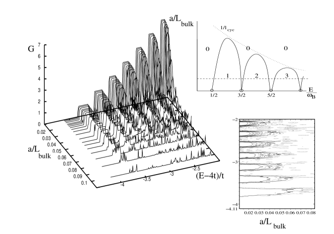
Figure 1: The conductance as function of energy for increasing values of the width $L_{\rm bulk}$ (left), and in a contour plot as function of energy and $L_{\rm bulk}$ (lower right), as compared with the schematic phase diagram (upper right). Finite integer values of the conductance correspond to the number of extended edge states. The disorder is uniformly distributed in an interval of width $W=0.8t$. There are $x=0.025$ magnetic flux quanta per elementary cell of area $a^{2}$.

Using the transfer matrix method, transfer we have calculated the 2-terminal conductancepmr92 $G$ as function of energy $E$ in a tight binding model with band width $8t$, where $t$ is the hopping amplitude, of a disordered quantum wire in a perpendicular magnetic field (Fig. 1), with hard wall boundary conditions at $y=\pm L_{\rm bulk}/2$ and finite length $L=2000a$.jetp Here we have assumed a square lattice with lattice spacing $a$. The disorder potential is uniformly distributed in an interval $[-W/2,W/2]$. These results are summarised in the phase diagram (Fig. 1), where the value of $G$, in units of $e^{2}/h$, is given as function of bulk width $L_{\rm bulk}$ and energy $E$ in units of $\hbar\omega_{B}$, for a disorder strength $W=0.8t$. As expected, $G=m$, where $m$ is the number of extended edge states between the Landau bands. Close to the middle of the Landau bands, however, the conductance plateaus collapse abruptly to $G=0$.

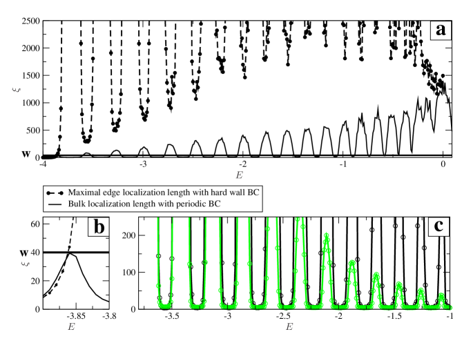
Figure 2: (Color online) (a) The localization length for a disordered wire calculated with the transfer matrix method with periodic boundary conditions (full line) and with hard wall boundary conditions (dashed line) for uniformly distributed uncorrelated disorder in an interval of width $W=0.8t$. The straight line indicates the bulk width $w=40a$. There are $x=0.025$ magnetic flux quanta per elementary cell of area $a^{2}$. (b) Enlargement of the low-energy region of (a). Edge and bulk localization length coincide as long as no edge state is present. (c) The functions $\xi_{\rm edge}/\xi(E)$ (black) and $e^{2w/\xi}$ (green).

When the wires are so narrow, that the edge states cannot form, as it is the case when the width is smaller than the cyclotron length, or when edge states of opposite chirality are mixed by backscattering, then all the states become localized and the conductance is vanishing with only small mesoscopic fluctuations due to the finite length $L$ of the wire. Previously, it has been pointed out that, when the bulk localization length $\xi$ is smaller than the physical wire width $w$, backscattering between edges is exponentially suppressed. As a result, the localization length of edge states increases strongly.

The overlap of opposite edge states is known to decrease exponentially with increasing wire width $w$ shkledge . Thus, the backscattering rate between edges, being proportional to the square of the overlap integral is $1/\tau\sim\exp(-2w/\xi)$. Since the edge states are one-dimensional, their localisation length due to the back scattering is given by $\xi_{edge}=2v_{F}\tau$, with Fermi velocity $v_{F}$. On the other hand, when the bulk localization length $\xi$ becomes equal to the wire width, one expects that the edge states become mixed with the bulk states, and localized with a length proportional to the bulk localization length $\xi$. Therefore, we conjectured the edge localization length to behave like jetp

$$\xi_{\rm edge}=\xi\exp(2w/\xi),$$ (1)

In Fig. 2a, the localization length is plotted as function of energy, as obtained with the transfer matrix method in a tight binding model of a disordered quantum wire in a perpendicular magnetic field with hard wall boundary conditions, dashed line. Since the edge states are the most extended states in the wire, this localisation length can be identified with the edge localisation length $\xi_{edge}$.

Using the transfer matrix method, transfer we have also calculated the localization length $\xi$ as function of energy $E$ for a disordered quantum wire with idendical properties, but with periodic boundary conditions, Fig. 2a, solid curve. Since there are no edge states this bulk localization length is small in the tails of Landau bands, and has maxima, which are seen to increase linearly with $n$.

Indeed the behavior of the edge state localisation length follows qualitatively the behaviour suggested by Eq. (1). The edge localization length does increase sharply, whenever the bulk localisation length becomes smaller than the wire width $w$ (full straight line). Note that the minima in the middle of the Landau bands do increase linearly with the Landau band number $n$. In Fig. 2c, we have explicitly plotted $\xi_{edge}/\xi$ and $\exp(2w/\xi)$, using the numerically calculated values for $\xi_{edge}$ and $\xi$, as function of $E$. We find that both functions coincide for all energies above the lowest Landau band and for $\l_{cyc}<w$, so that edge states exist in the tails of the Landau bands.

An abrupt decrease of the inverse localisation length has been found before for energies in the upper tail of the lowest Landau level and the tails of the second Landau level in Ref. 8. In agreement with our above results, it has been found there, that the inverse localisation length decays exponentially in the tails, like $1/\xi_{edge}\sim\exp(-\beta(E)w)$. The fitted values of $\beta$ have been found there to depend weakly on energy, whereas we identified it directly with the energy dependent inverse bulk localisation length $1/\xi(E)$.

From these results we can conclude that the energy at which edges states backscatter and become localized, is, given by the condition that the bulk localization length is on the order of the wire width, $\xi(E_{m,p})=w$. At this energy, $m$ edge states mix and transitions from extended edge states to insulating states occur. This causes sharp jumps of $G$ from finite integer to vanishingly small values, as seen in Fig. 1. This can be explained by the exponential decrease of the edge state localization length, Fig. 2. We note that $m=n$ when the energy is above the $n$-th Landau band , whereas $m=n-1$, if it is below.

A more detailed understanding of this drastic behaviour of the conductance can be obtained by considering the dimensional crossover of the bulk localization length in disordered wires. crossover ; jetp In a 2DES with broken time reversal symmetry, scaling theory ab ; weg ; hikami ; elk and numerical scaling studies mk81 ; transfer find that the bulk localization length $\xi$ is independent of the wire width, $\xi_{\rm 2D}=l_{0}\,\exp(\pi^{2}g^{2})$. Here, $g$, is the 2D conductance parameter per spin channel. $l_{0}$ is the short distance cutoff, the elastic mean free path $l=2g(B=0)/k_{{\rm F}}$ ($k_{\rm F}$ Fermi wave number) at weak magnetic fields, $b\equiv\omega_{B}\tau<1$. For stronger magnetic fields, $b>1$, the short length scale $l_{0}$ becomes the cyclotron length $l_{\rm cyc}$. The conductance parameter $g$ exhibits Shubnikov-de-Haas oscillations as function of magnetic field for $b>1$. Maxima occur when the Fermi energy is in the center of Landau bands. The localization length in tails of Landau bands, where $g\ll 1$ is very small, is of the order of the cyclotron length $l_{\rm cyc}=v_{F}/\omega_{B}=\sqrt{2n+1}l_{B}$. It increases towards the centers of the Landau bands, $E_{n0}=\hbar\omega_{B}(n+1/2)$ ($n=0,1,2,...$), with $\omega_{B}=eB/m^{*}$ the cyclotron frequency ($e$ elementary charge, $m^{*}$ effective mass), $v_{F}$ the Fermi velocity, and $l_{B}^{2}=\hbar/eB$ defines the magnetic length. In an infinite 2DES in perpendicular magnetic field, the localization length at energy $E$ diverges as $\xi\sim|E-E_{n0}|^{-\nu}$. The critical exponent $\nu$ is known from numerical finite size scaling studies for the lowest two Landau bands, $n=0,1$, to be $\nu=2.33\pm 0.04$ for spin-split Landau levels, hucke ; huckerev in agreement with analytical raikh and experimental studies scalingexp . In a finite 2DES, a region of state exists in the centers of disorder broadened Landau-bands, which cover the whole system of size $L$. The width of these regions is given by $\Delta E=(l_{\rm cyc}/L)^{1/\nu}\Gamma$, where $\Gamma=\hbar(2\omega_{B}/\pi\tau)^{1/2}$ is the band width, with elastic scattering time $\tau$.

However, the 2D localization length is seen to increase strongly from band tails to band centers, even when the wire width $w$ is so narrow, that it is far from the critical point at $w\rightarrow\infty$. One can estimate the noncritical localization length for uncorrelated impurities, by inserting $g$, as obtained within self consistent Born approximation. ando Its maxima are $g(E=E_{n0})=(2n+1)/\pi=g_{n}$. Thus, $\xi_{\rm 2D}(E_{n0})=l_{\rm cyc}\exp{(\pi^{2}g_{n}^{2})}$ are macroscopically large in centers of higher Landau bands, $n>1$. huckerev ; levitation When the width of the system $w$ is smaller than $\xi_{\rm 2D}$, electrons in centers of Landau bands can diffuse between the edges of the system. In long wires, however, the electrons are localized due to quantum interference along the wire with a localization length that is found to depend linearly on $g$ and $w$, ef ; larkin ; dorokhov ; jetp

$$\xi_{\rm 1D}=2g(B)w.$$ (2)

The conductance per spin channel, $g(b)=\sigma_{xx}(B)/\sigma_{0}$, is given by the Drude formula $g(b)=g_{0}/(1+b^{2})$, ($g_{0}=E\tau/\hbar$, $b=\omega_{B}\tau$) for weak magnetic field, $b<1$. For $b>1$, when the cyclotron length $l_{\rm cyc}$ is smaller than the mean free path $l$, disregarding the overlap between Landau bands, $g$ is obtained in SCBA, ando $g(B)=(1/\pi)(2n+1)(1-(E_{\rm F}-E_{n})^{2}/\Gamma^{2}),$ for $\mid E-E_{n}\mid<\Gamma$. One obtains the localization length for $b>1$ and $\mid\epsilon/b-n-1/2\mid<1$ by inserting $g$. It oscillates between maximal values in centers of Landau bands, and minimal values in band tails. For $n>1$, one finds in band centers,

$$\xi_{n}=\frac{2}{\pi}\left(2n+1\right)w\left[1-\frac{\ln\sqrt{1+\left(w/l_{\rm cyc}\right)^{2}}}{(n+1/2)^{2}}\right]^{1/2}.$$ (3)

Thus, the localization length in the center of Landau bands is found to increase linearly with Landau band index $n$. This is exactly the behaviour observed above in the numerical results, Fig. 2.

While it is reasonable to conclude that the edge states do mix with the bulk states at the energy where the bulk localization length is equal to the wire width, and the electrons diffuse freely from edge to edge but are localized along the wire, the question arises, how exactly this transition from extended edge states to localized states does occur. One can gain some further insight by connecting the two ends of the wire together to form an annulus. Piercing magnetic flux through the annulus affects only states whose localization length is larger than the circumference of the annulus. Guiding centers of those states which extend around the annulus do shift in position and energy halperin with a change in magnetic flux. As shown above, in the middle of the Landau band, the electrons can diffuse freely from edge to edge, but are localized along the annulus with $\xi>w$. When adiabatically changing the magnetic flux, the energy of an edge state changes continously. However, it cannot enter the band of localized states, so that at the energy $E_{m}$, with $\xi(E_{m})=w$, the edge state must be transfered to the opposite edge. There it moves up in energy when the magnetic flux is increased further. halperin

In the following, we study the states at this transition in detail in order to find out, whether the edge states become localized mainly by mixing completely with the bulk states, or rather the transition from extended chiral edge states to localized states occurs due to the nonlocal coherent superposition of edge states with opposite chirality, located at opposite edges.

III Exact diagonalization

In this chapter, we study the localization properties of electrons in quasi one-dimensional wires in the presence of disorder and a strong magnetic field by means of exact diagonalization.

III.1 The model

The Hamiltonian of the quasi-1D-wire in the presence of a disorder potential $V_{\rm dis}$ and a confinement potential $V_{\rm conf}$, is given by

$$H=\frac{1}{2m^{\ast}}\left({\bf p}-e{\bf A}\right)^{2}+V_{\rm dis}({\bf r})+V_{\rm conf}({\bf r})\;,$$ (4)

where $e>0$ is the elementary charge and $m^{\ast}$ the effective electron mass.

The disorder potential is modelled as

$$V_{\rm dis}({\bf r})=\sum\limits_{i=1}^{N_{\rm imp}}V_{i}\delta({\bf r}-{\bf r}_{i}),$$ (5)

where $N_{\rm imp}$ is the number of impurities with uniformly distributed amplitude $V_{i}\in[-V_{0},V_{0}]$. ${\bf r}_{i}$ is the random position of the impurity.

As we seek to investigate the interplay and localization of edge states and bulk states in a quantum wire, we assume periodic boundary conditions in the $x$-direction along the wire and choose

$$V_{\mbox{\footnotesize conf}}(y)=\left\{\begin{array}[]{cc}\frac{1}{2}m\omega_{p}^{2}(y-L_{\rm bulk}/2)^{2}&y\geq L_{\rm bulk}/2\\ 0&-\frac{1}{2}L_{\rm bulk}<y<\frac{1}{2}L_{\rm bulk}\\ \frac{1}{2}m\omega_{p}^{2}(y+L_{\rm bulk}/2)^{2}&y\leq-L_{\rm bulk}/2\end{array}\right.$$ (6)

as confinement potential in the transversal direction (see Fig. 3). This model allows us to tune the confinement strength with the parameter $\omega_{p}$. The wire width is now defined by the bulk width $L_{\rm bulk}$. In the limit $L_{\rm bulk}=L$, we get the usual 2D model for the Quantum Hall effect Ando , while for $L_{\rm bulk}=0$ we have the parabolic wire model hajdubook . In the limit of large confinement frequency $\omega_{p}>\omega_{c}$, one approaches hard-wall boundary conditions.

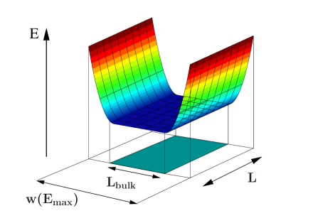
Figure 3: (Color online) Model of a quantum wire with length $L$, parabolic confinement and finite bulk region of width $L_{\rm bulk}$. The physical width $w(E_{\rm max})$ is indicated, where $E_{\rm max}$ is the largest energy considered.

This type of confinement provides a smooth transition between the edge potential and the potential-free bulk region and renders the situation in real wires better than assuming hard wall boundaries.

The physical width $w$ of parabolic wires $w$ is a function of the Fermi energy $E$,

$$w(E,L_{\rm bulk})=2\;\sqrt{\frac{2E-\hbar\Omega}{\hbar\omega_{B}}}\;\frac{\omega_{B}}{\omega_{p}}\;l_{B}+L_{\rm bulk},$$ (7)

with $\Omega=\sqrt{\omega_{p}^{2}+\omega_{B}^{2}}$. It is obtained by finding the energy eigenvalue of the clean wire which is equal to $E$ and has its guiding center at $\pm w/2$. We fix the basis width $L_{\rm basis}$ to be larger than the physical width $w(E_{\rm max})$ at the highest considered energy $E_{\rm max}$. The total number of magnetic flux quanta in the model system is then fixed to $N_{\phi}=L_{\rm basis}L/(2\pi l_{B}^{2})$.

III.2 Wavefunction analysis

The Hamiltonian, Eq. (4) is diagonalized in the Landau representation with basis functions

$$\left\langle\bf r\right|nX\rangle=\frac{1}{\left(l_{B}L\sqrt{\pi}2^{n}n!\right)^{1/2}}\mathrm{e}^{-\frac{(y-X)^{2}}{2l_{B}^{2}}}H_{n}\left(\frac{y-X}{l_{B}}\right)\;{\mathrm{e}}^{-\frac{iXx}{l_{B}^{2}}}$$ (8)

Here we have assumed the Landau gauge for the vector potential. The matrix elements of the confinement potential in the Landau representation are given in Appendix A.

The exact diagonalization of the Hamiltonian (4) yields eigenenergies $E_{\alpha}$ with corresponding wavefunctions

$$\psi_{\alpha}({\bf r})=\sum\limits_{nX}\left\langle\bf r\right|nX\rangle\langle nX\left|\alpha\right\rangle$$ (9)

The spatial extention of these wavefunctions is characterized by their participation ratio

$$P_{\alpha}=\left(L_{\rm bulk}L\int d^{2}r|\psi_{\alpha}({\bf r})|^{4}\right)^{-1},$$ (10)

which is small for localized states and large for extended states. Note that in this definition, $P_{\alpha}$ relates to the fixed bulk area $L_{\rm bulk}L$ while the wave functions can cover a larger area due to the smooth confinement, so that $P_{\alpha}>1$ is possible for all states.

In clean 2D systems all states in a Landau level are degenerate. In a disordered wire this degeneracy is lifted by the disorder, and at the edges by the confinement potential. Therefore, localized states in the tail of the Landau bands in the bulk region near the center of the wire coexist with states at the edges at the same energy, and, in principle, mixing of states from the bulk with edge states is possible.

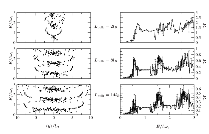
Figure 4: Left: The energy eigenvalues $E_{\alpha}$ of all states in a wire of length $L=40.1l_{B}$ in a perpendicular magnetic field of 8 T for three different bulk widths are plotted versus the expectation value of the transversal position, $\langle\alpha\mid y\mid\alpha\rangle$. The disorder amplitude is fixed to $V_{0}=0.73\hbar\omega_{c}$ with $N_{i}=150$ impurities and the confinement energy is chosen to have the same magnitude with $\hbar\omega_{p}=0.73\hbar\omega_{c}$. The basis width is chosen as $L_{\mathrm{basis}}=1.5~{}w(E_{\rm max})$, Eq. (7), with $E_{\rm max}=2\hbar\omega_{c}$. Right: Corresponding participation ratio $P_{\alpha}$ versus $E_{\alpha}$.

These features are clearly seen in the left part of Fig. 4. For a wire of length $L=40.1l_{B}$ in a perpendicular magnetic field of $B=8\mathrm{T}$, corresponding for $m^{\ast}=0.067$ in units of the bare electron mass to $\hbar\omega_{c}=13.82$ meV, for three different bulk widths $L_{\rm bulk}$ the eigenenergies are plotted versus the expectation value of their transversal position, $\langle\alpha\mid y\mid\alpha\rangle$. Although we have chosen a smooth confinement potential, these results are in good agreement with earlier results with short ranged disorder in Ref. ohtsuki, . Obviously, the edge states between the Landau bands are hardly affected by the disorder potential. There is a coupling of edge states of the same chirality in the second and higher Landau bands which leads to the formation of minibands in between the Landau band, ohtsuki as seen most clearly in Fig. 5. There, we show the same quantities for a longer system with $L=100l_{B}$ and $L_{\rm bulk}=8l_{B}$ at $B=8$ T. The disorder is realized by 400 scatterers with $V_{0}=0.73\;\hbar\omega_{c}$, with the same value as the confinement energy $\hbar\omega_{p}=0.73\;\hbar\omega_{c}$. However, there is an abrupt shift of the center of the eigenstates towards the middle of the wire, when their energy is approaching the middle of the Landau band. Still, one can not conclude, if this fact is mainly due to the backscattering between edge states from opposite edges, having opposite chirality, or if it is mainly due to a mixing with the bulk localized states.

In order to learn more about the nature of these states, we have calculated the Frmi energy dependence of the participation ratio for different bulk widths with fixed disorder potential and constant magnetic field as shown in the right part of Figs. 4, 5. It is observed for all three widths that the participation ratio and the eigenenergies, fluctuate as a result of disorder especially in the center of the wire. The participation ratio increases with energy in the tails of the Landau bands and reaches a maximum close to the corresponding center energy (between $0.5\;\hbar\omega_{c}$ for $L_{\rm bulk}\rightarrow\infty$ and $0.5\;\hbar(\omega_{c}^{2}+\omega_{p}^{2})^{1/2}$ for $L_{\rm bulk}\rightarrow 0$). The participation ratio saturates to a constant value between the Landau bands, where only edges states exist, as confirmed by comparison with the left side of Fig. 4.

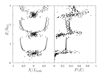
Figure 5: Energy dispersion $E(X)$ and corresponding participation ratio $P(E)$ for a longer system with $L=100l_{B}$ and $L_{\rm bulk}=8l_{B}$ at $B=8$ T. The disorder is realized by 400 scatterers with uniformally distribted amplitude with maximal value, $V_{0}=0.73\;\hbar\omega_{c}$, which equals the confinement energy $\hbar\omega_{p}=0.73\;\hbar\omega_{c}$.

In the following, we scrutinize the localization behaviour in the different energy regions identified above by the energy dispersion and the participation ratio. To determine the nature of the states, we plot the basis state contributions and spatially resolved probabilities for a sample with $L=100l_{B}$ and $L_{\rm bulk}=8l_{B}$ at typical energies, with disorder amplitude and confinement energy comparable to the cyclotron energy. We concentrate on the lowest Landau level and investigate wavefunctions at energies in characteristic regions of the participation ratio. The result is displayed in figure 6.

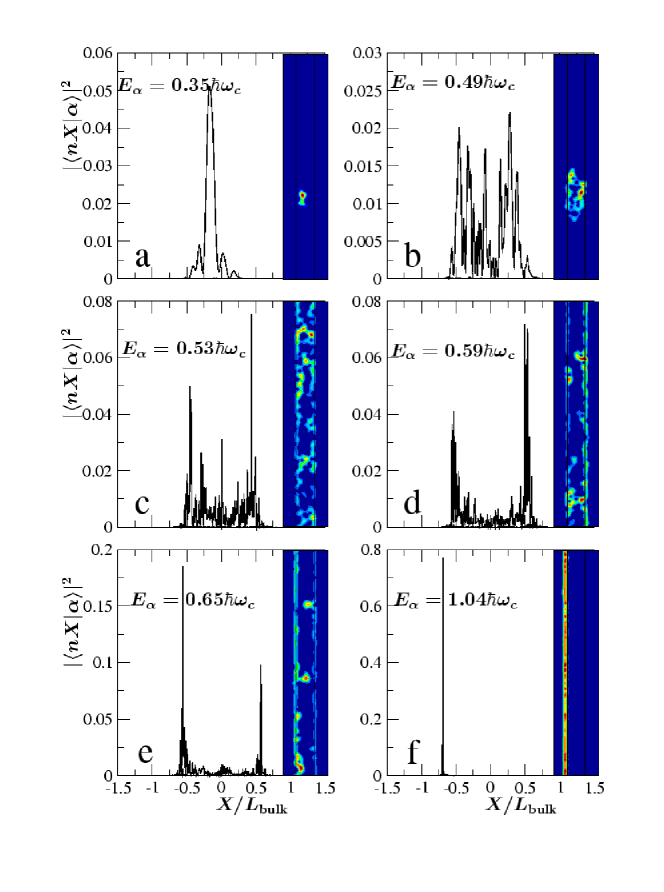
Figure 6: (Color online) Basis state contributions to eigenstates at selected energies. The right insets show the correponding probability densities (blue for low, red for high values), solid lines mark the bulk region. System parameters are the same as in Fig. 5.

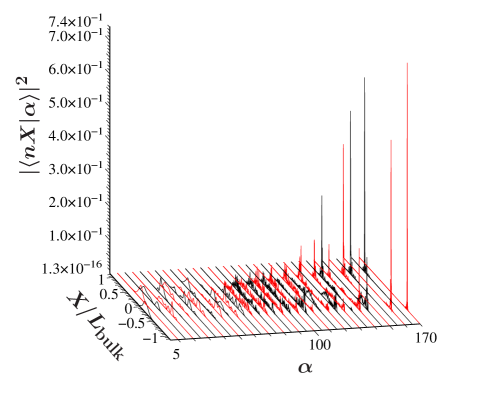
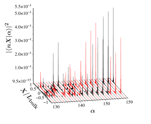
Figure 7: (Color online) Basis state contributions $|\left\langle nX\right|\alpha\rangle|^{2}$ to eigenstates $\alpha$ at different energies (a) for every fifth state in the lowest Landau level, (b) for every state with energy between $0.6\;\hbar\omega_{c}$ and $0.8\;\hbar\omega_{c}$. System parameters are the same as in Fig. 5. Different colors are used for adjacent curves in order to distinguish them clearly.

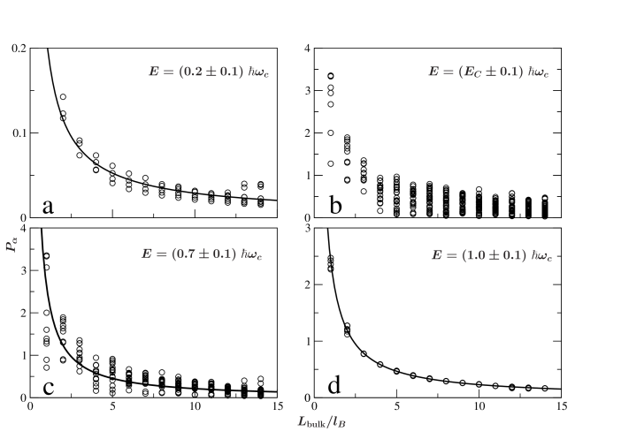
Figure 8: Participation ratio in dependence of bulk width for different energies. $E_{C}$ is determined for each bulk width as the energy, at which the system reaches the maximal participation ratio in the lowest Landau band. System parameters are the same as in Fig. 4. Solid lines are fitting functions: (a) $P_{\alpha}=0.21\,(L_{\rm bulk}/l_{B})^{-0.86}$, (c) $P_{\alpha}=2.62\,(L_{\rm bulk}/l_{B})^{-1.09}$, (d) $P_{\alpha}=2.41\,(L_{\rm bulk}/l_{B})^{-1.02}$.

We find states at $E=0.3\hbar\omega_{c}$ (Fig. 6a) which are 2D localized, as confirmed by the fact that they have contributions from basis states with guiding centers in the bulk region, only. In the band center around $E=0.5\hbar\omega_{c}$ the participation ratio fluctuates strongly. In this region we find 2D localized states as well as 1D localized states with a localization length larger than the bulk width, but much smaller than the wire length (Fig 6b). In the latter case, basis states from bulk and edge region mix with comparable contributions. Furthermore, we can identify states which cover the whole sample, as shown in Fig 6c. These states couple to all regions as well, although the contributions from the left and right edges seem to prevail slightly. The trend indicated by the maxima close to the edges intensifies in the transition region (Fig. 6d). At a specific energy, the contribution of the bulk states is small compared to the sharp maxima at the edges, while the electron is found with the same probability on the right or  the left edge of the wire (Fig. 6e). We believe that this nonchiral edge state is unique at least in the thermodynamic limit, of $w\rightarrow\infty$ and governs the new type of metal-insulator transition, the CMIT, in quasi-1D quantum Hall wires. This state exhibits notable localization features: being an edge state concerning the participation ratio, it has to be considered localized concerning the conductance, since current flows with equal probability, but reversed sign on both edges. This behaviour is consistent with the sudden breakdown of the conductance observed in Fig. 1.

At higher energies, below the next Landau band, edge states are formed as seen in Fig. 6. These states are found to be insensitive to disorder.

This sequence of transitions from 2D bulk states, quasi-1-D localized states, states with peaks on both edges of the wire, and decoupled edge states is visible in Fig. 7a, where we show the basis state contributions for every fifth state in the lowest Landau level. All features discussed above are seen clearly, with a remarkably narrow transition region from 1D localized states to edge states, as one moves from state 125 to state 145.

In order to visualize this transition in detail, we plot in this interval all states in Fig. 7b. The higher energy states are clearly edge states, which are decoupled from the bulk, and are altenatingly located either on the left or on the right side of the wire. The lower the energy, the smaller becomes that peak in intensity at the edge. Still, each state stays located in the edge region, with only a small coupling to the nearest part of the bulk. Then, suddenly, at state ($\alpha=143$ in Fig. 7), there appear two peaks of comparable amplitude on both edges, while the contribution of the bulk is still small. All states $\alpha=139-143$ share the two pronounced peak at the edges, while the bulk contribution increaes only slowly with lowering the energy. Before the transition to quasi-1D-states with more or less uniform distribution across the bulk, there is a reappearance of edge like states $\alpha=135-138$, which we attribute to mesoscopic fluctuations due to the random distribution of disorder in this rather mesoscopic sample. The transition which we observed here happens thus rather smooth as compared to the sharp transitions in the transfer matrix results shown in Fig. 1. This can be attributed to the fact that the finite system with $L=100l_{B}$ which we have diagonalized here is much smaller than the system which was handled by the transfer matrix method. As expected far away from the thermodynamic limit, $L,w\rightarrow\infty,L/w={\rm const.}$, the transition occurs in a finite energy interval rather than at a single point. Finite size effects can be revealed further by studying the dependence of the states on the bulk width.

To this end we next study the system size dependence of the participation ratio. Fig. 8 shows the participation ratio of all states in a given energy interval for systems with different bulk widths $L_{\rm bulk}$. Disorder configuration, wire length and confinement energy $\hbar\omega_{p}$ are kept fixed for all the systems. As a characteristic example for the behaviour in the low energy region, we investigate states in an interval around energy $E=0.2\hbar\omega_{c}$ (Fig. 8a). In this region, the participation ratio scales with the wire width approximately as $P\propto L_{\rm bulk}^{-1}$. This is in agreement with the expected scaling of 2D localized states which give a contribution $\psi_{\alpha}^{2}\propto 1/\xi_{2D}^{2}$, only within a localization area $\xi_{2D}^{2}$ where $\xi_{2D}$ is the 2D localization length of the wavefunction, which is independent of the wire length $L$ and width $L_{\rm bulk}$. It follows that,

$$P_{2D}\propto\xi_{2D}^{2}L^{-1}L_{\rm bulk}^{-1}\ll 1,$$ (11)

in good agreement with Fig. 8a.

The behaviour changes in the center of the Landau band (Fig. 8b). There, the density of states is higher, and the disorder results in a wide range of participation ratios. For large bulk widths, $L_{\rm bulk}>5l_{B}$, the range of participation ratios becomes constant and saturates to a finite value. Note that quasi-1-D localized states cover approximately an area $L_{\rm bulk}\xi_{1D}\sim gL_{\rm bulk}^{2}$, and contribute in this area with probability density $\psi_{\alpha}^{2}\sim 1/(\xi_{1D}L_{\rm bulk})$. As a result, one expects for quasi-1-D localized states, according to Eq. (2),

$$P_{1D}\propto\frac{\xi_{1D}}{L}\sim g\frac{L_{\rm bulk}}{L},$$ (12)

increasing linearly with $L_{\rm bulk}$. When the wire is comparable or shorter than the quasi-1D localization length, however, the participation rato shows rather the behavior of 2D extended states which cover the whole wire area $Lw$ with probability density $1/(Lw)$, yielding the typical participation rato of extended states

$$P_{ext}\sim w/L_{\rm bulk}=\mathrm{const}>1,$$ (13)

being independent of the width $L_{\rm bulk}$. Note that for extended statesone would expect $P_{\alpha}=w/L_{\rm bulk}$, which according to equation (7) converges to 1 for $L_{\rm bulk}\rightarrow\infty$. Whereas $P_{\alpha}$ in Fig. 8b is indeed seen to saturate to a constant mean value, this value is found not to exceed 1. This is consistent with the fact that the wavefunction is multifractal.klesse

The scaling of the participation ratios in the high energy tail of the lowest Landau band (Fig. 8c,d) is again a power law $P\propto L_{\rm bulk}^{-1}$, but with an absolute value much larger than in Fig. 8a. This resembles the expected feature for edge states, which cover an area $l_{B}L$ with probability density $1/(l_{B}L)$, yiedling,

$$P_{\rm edge}\propto l_{B}/L_{\rm bulk},$$ (14)

which is both in magnitude and in the functional dependence on $L_{\rm bulk}$ in good agreement with Fig. 8d. Note that in the transition region, Fig. 8c, the large mesoscopic fluctuations do not allow to distinguish characteristic features of the nonchiral edge states at the transition, the functional dependence on $L_{\rm bulk}$ is that expected for edge states and localized bulk states alike, which both coexist in this energy region, as we had seen above in Fig. 7.

In summary, our model allows to study the mutual influence between the states in the bulk region, where the influence of the disorder potential is strong, and states in the edge region, where the confinement potential prevails. We found that in the narrow energy region of the CMIT the disorder-induced coupling between the edges creates nonchiral edge states which have comparable weights on both edges, but only a negligible mixing with the bulk.

IV Conclusions

We conclude, that in quantum Hall bars of finite width $w\ll\xi_{n}$ at low temperatures quantum phase transitions occur between extended chiral edge states and a quasi-1D insulator. These are driven by the crossover from 2D to 1D localization of bulk states. These metal-insulator transitions resemble first-order phase transitions in the sense that the localization length abruptly jumps between exponentially large and finite values, which we confirmed by calculating the edge state localization length, explicitly. In the thermodynamic limit, fixing the aspect ratio $c=L/w$, when sending $L\rightarrow\infty$, then $c\rightarrow\infty$, the two–terminal conductance jumps between exactly integer values and zero. The transitions occur at energies where the localization length of bulk states is equal to the geometrical wire width. Then, $m$ edge states mix and electrons are free to diffuse between the wire boundaries but become Anderson localized along the wire. Close to that transition we found with exact diagonalisation studies that particular states exist, which are superpositions of edge states with opposite chirality, with an order of magnitude smaller bulk contribution. Although this state is located at the edges, it is a nonlocal state, having comparable weights on opposite sides of the sample. Thus, it can have a mesoscopic extension across the width of the Hall bar, if it is more narrow than the phase coherence length. The Chiral Metal–Insulator Transition is of mesoscopic nature since, at finite temperature, the phenomenon of the CMIT can only be observed, when the phase coherence length exceeds the quasi-1D localization length in centers of Landau bands, $L_{\varphi}>\xi_{n}$. One then should observe transitions of the two-terminal resistance from integer quantized plateaus, $R_{n}=h/ne^{2}$ to a Mott variable-range hopping regime of exponentially diverging resistance. Such experiments would yield information about the coupling between edge and bulk states in quantum Hall bars. At higher temperature, when $L_{\varphi}<\xi_{n}$, the conventional form of the integer quantum Hall effect is recovered klitzing .

We have studied the modification of the CMIT by correlations in the disorder potential and due to interactions. These results will be presented in a subsequent publication.

Acknowledgments We acknowledge useful discussions with M. E. Raikh, A. MacKinnon, and B. Huckestein. This research was supported by German Research Council (DFG), Grant No. Kr 627/10, Schwerpunkt ”Quanten-Hall-Effekt”, and by EU TMR-network Grant. No. HPRN-CT2000-0144.

Appendix A Matrix elements for confinement in Landau representation

The matrix element of the confinement potential defined by equation (6) in Landau representation $\left\langle nX\right|V_{\mbox{\footnotesize conf}}\left|n^{\prime}X^{\prime}\right\rangle$ is given by

$$\left\langle nX\right|V_{\mbox{\footnotesize conf}}\left|n^{\prime}X^{\prime}\right\rangle=\delta_{XX^{\prime}}\frac{1}{\sqrt{\pi}l_{B}2^{(n+n^{\prime})}n!n^{\prime}!}\left[M_{nn^{\prime}}\left(\frac{L_{\rm bulk}}{2},X\right)+(-1)^{(n+n^{\prime})}M_{nn^{\prime}}\left(\frac{L_{\rm bulk}}{2},-X\right)\right],$$ (15)

and

$$M_{nn^{\prime}}\left(\frac{L_{\rm bulk}}{2},X\right) = \int\limits_{L_{\rm bulk}/2}^{\infty}dy\,\,\mathrm{e}^{-\frac{(y-X)^{2}}{l_{B}^{2}}}H_{n}\left(\frac{y-X}{l_{B}}\right)H_{n^{\prime}}\left(\frac{y-X}{l_{B}}\right)\left(\frac{y-L_{\rm bulk}/2}{l_{B}}\right)^{2}$$ (16)

$$= l_{B}\int\limits_{b}^{\infty}d\xi\,\,\mathrm{e}^{-\xi^{2}}(\xi-b)^{2}H_{n}(\xi)H_{n^{\prime}}(\xi)\;\;,$$ (17)

where $\xi=(y-X)/l_{B}$ and $b=(L_{\rm bulk}/2-X)/l_{B}$.

By expanding all polynomials in Eq. (17) in monomials in $\xi$ using the relation

$$H_{n}(\xi)=n!\sum\limits_{m=0}^{[\frac{n}{2}]}(-1)^{m}\frac{2^{n-2m}}{m!(n-2m)!}\xi^{n-2m},$$ (18)

where $[x]$ denotes the largest integer smaller than $x$, one gets

$$M_{nn^{\prime}}(b,X) = l_{B}\,\,n!n^{\prime}!\sum\limits_{l=0}^{[\frac{n}{2}]}\sum\limits_{k=0}^{[\frac{n^{\prime}}{2}]}\Biggl{[}(-1)^{l+k}\frac{2^{n-2l+n^{\prime}-2k}}{l!k!(n-2l)!(n^{\prime}-2k)!}$$

$$\times \left(f^{(2+n-2l+n^{\prime}-2k)}(b)-2bf^{(1+n-2l+n^{\prime}-2k)}(b)+b^{2}f^{(n-2l+n^{\prime}-2k)}(b)\right)\Biggr{]}$$

In the last expression,

$$f^{(M)}(b)=\int\limits_{b}^{\infty}d\xi\,\,\xi^{M}\mathrm{e}^{-\xi^{2}}=\frac{M-1}{2}f^{(M-2)}(b)+b^{M-1}\frac{1}{2}\mathrm{e}^{-b^{2}}$$ (19)

This recursive formula can be obtained by repeated partial integration and is valid for even and odd $M>1$. An explicit evaluation requires the inital expressions

$$f^{(0)}(b) = \frac{1}{2}\mathrm{e}^{-b^{2}}$$ (20)

$$f^{(1)}(b) = \frac{1}{2}\sqrt{\pi}\;\mbox{\rm erfc}(b)\,\,,$$ (21)

with the complementary error function

$$\mbox{\rm erfc}(b)=\int\limits_{b}^{\infty}d\xi\,\,\mathrm{e}^{-\xi^{2}}.$$ (22)

References

- (1) B. I. Halperin, Phys. Rev. B 25, 2185 (1982).
- (2) R. J. Haug and K. von Klitzing, Europhys. Lett. 10, 489 (1989).
- (3) G. Timp, et al., Phys. Rev. Lett. 59, 732 (1987); ibid. 63, 2268 (1989); E. Peled, D. Shahar, Y. Chen, D. L. Sivco and A. Y. Cho, Phys. Rev. Lett. 90, 246802 (2003).
- (4) T. Ando , Phys. Rev. B 49, 4679 (1994).
- (5) B. J. van Wees, et al., Phys. Rev. B 43, 12431 (1991).
- (6) B. I. Shklovskii, Pis’ma Zh. Eksp. Teor. Fiz. 36, 43 (1982) [ JETP Lett. 36, 51 (1982)]; A. V. Khaetskii and B. I. Shklovskii, Zh. Eksp. Teor. Fiz. 85, 721 (1983) [Sov. Phys. JETP 58, 421 (1983)]; M. E. Raikh and T. V. Shahbazyan, Phys. Rev. B 51, 9682 (1995).
- (7) T. Ohtsuki and Y. Ono, Solid State Commun. 65, 403 (1988); Solid State Commun. 68, 787 (1988). Y. Ono, T. Ohtsuki, and B. Kramer, J. Phys. Soc. Jpn. 58, 1705 (1989); T. Ohtsuki and Y. Ono, J. Phys. Soc. Jpn. 58, 956 (1989);
- (8) T. Ando, Phys. Rev. B 42, 5626 (1990).
- (9) R. G. Mani and K. v. Klitzing, Phys. Rev. B 46, 9877 (1992); R. G. Mani, K. von Klitzing, and K. Ploog, Phys. Rev. B 51, 2584 (1995).
- (10) P. G. N. d. Vegvar, et al., Phys. Rev. B 36, 9366 (1987).
- (11) M. L. Roukes, et al., Phys. Rev. Lett. 59, 3011 (1987).
- (12) S. Kettemann, B. Kramer, and T. Ohtsuki, JETP Lett. 80, 316 (2004).
- (13) B. Kramer and A.MacKinnon, Rep. Prog. Phys. 56, 1469 (1993).
- (14) J. B. Pendry, A. MacKinnon, and P. J. Roberts, Proc. R. Soc. London A437, 67 (1992).
- (15) S. Kettemann, J. Phys. Soc. Jpn. Suppl. A 72, 197 (2003); S. Kettemann, Phys. Rev. B 69, 035339 (2004).
- (16) E. Abrahams, et al. Phys. Rev. Lett 42 673(1979).
- (17) F. Wegner, Z. Physik B 36,l209(1979); Nucl. Phys. B 316, 663(1989)
- (18) S. Hikami, Prog. Theor. Phys. 64, 1466 (1980).
- (19) K. B. Efetov, A. I. Larkin, and D. E. Khmel’nitskii, Zh. Eksp. Teor. Fiz. 79, 1120(1980) [Sov. Phys. JETP 52, 568(1980)].
- (20) A. MacKinnon and B. Kramer, Phys. Rev. Lett. 47, 1546 (1981); Z. Phys. B 53, 1 (1983).
- (21) J. T. Chalker and G. J. Daniell, Phys. Rev. Lett. 61, 593 (1988); B. Huckestein and B. Kramer, Phys. Rev. Lett. 64, 1437 (1990)
- (22) B. Huckestein, Rev. Mod. Phys. 67, 357 (1995).
- (23) T. Ando and Y. Uemura, J. Phys. Soc. Jpn. 36, 959 (1974); T. Ando, J. Phys. Soc. Jpn. 36 1521 (1974); T. Ando, J. Phys. Soc. Japan 37, 622 (1974).
- (24) A. G. Galstyan and M. E. Raikh, Phys. Rev. B 56, 1422 (1997); D. P. Arovas, M. Janssen, and B. Shapiro, Phys. Rev. B 56, 4751 (1997).
- (25) H. P. Wei, et al. Phys. Rev. Lett. 61, 1294 (1988); S. Koch, et al., Phys. Rev. Lett. 67, 883 (1991); L. W. Engel, et al., Phys. Rev. Lett. 71, 2638 (1993); M. Furlan, Phys. Rev. B 57, 14818 (1998); F. Hohls, et al., Phys. Rev. Lett. 88, 036802 (2002).
- (26) B. Huckestein, Phys. Rev. Lett. 84, 3141-3144 (2000).
- (27) K. B. Efetov, Supersymmetry in Disorder and Chaos Cambridge University Press, Cambridge (1997).
- (28) K. B. Efetov and A. I. Larkin, Zh. Eksp Teor. Fiz. 85, 764(1983) ( Sov. Phys. JETP 58, 444 ).
- (29) O. N. Dorokhov, Pis’ma Zh. Eksp. Teor. Fiz. 36, 259 (1982)) [JETP Lett. 36, 318 (1983)];, Zh. Eksp. Teor. Fiz. 85, 1040 (1983) [ Sov. Phys. JETP 58, 606 (1983)]; Solid State Commun. 51, 381 (1984).
- (30) T. Ando, J. Phys. Soc. Jpn. 53, 3126 (1984)
- (31) M. Janßen, O. Viehweger, U. Fastenrath, and J. Hajdu, Introduction to the Theory of the Integer Quantum Hall Effect, VCH-Verlagsgruppe, Weinheim, Germany (1994)
- (32) K. Takashima, et al., Physica E 20, 160 (2003). ed. by S. Das Sarma and A. Pinczuk, Wiley New York (1997).
- (33) K. von Klitzing, G. Dorda, and M. Pepper, Phys. Rev. Lett. 45, 494 (1980).
- (34) W. Pook and M. Janssen, Z. Phys. B 82, 295 (1991); B. Huckestein, B. Kramer, and L. Schweitzer, Surf. Sci. 263 125 (1993); B. Huckestein and R. Klesse, Phys. Rev. B 55, R7303 (1997)