Resonator design for surface electron lifetime studies using scanning tunneling spectroscopy

Abstract

We derive expressions for the lossy boundary-scattering contribution to the linewidth of surface electronic states confined with atomic corrals and island resonators. Correcting experimentally measured linewidths for these contributions along with thermal and intrumental broadening enables intrinsic many-body lifetimes due to electron-electron and electron-phonon scattering to be determined. In small resonators lossy-scattering dominates linewidths whilst different scaling of widths and separations cause levels to merge in large resonators. Our results enable the design of resonators suitable for lifetime studies.

I Introduction

The dynamics of hot electrons and holes at surfaces have attracted considerable attention in recent years, not least due to their importance in photochemistry and charge-transfer processes such as electronically-induced adsorbate reactions. A particular focus has been the study of quasiparticle lifetimes associated with excitations in the band of surface-localised electronic states found at the (111) surfaces of the noble metals, which have become a testing ground for new theoretical, computational and experimental methods aimed at developing a deeper fundamental understanding of quasiparticle dynamics. ech04_ Theoretically, much progress has been made towards a quantitative account of inelastic electron-electron kli00a ($e$-$e$) and electron-phonon eig02_ ($e$-$p$) interactions of these states, whilst techniques such as scanning tunneling microscopy bur99_ ; bra02_ (STM) and spectroscopy jli98c (STS), and photoelectron spectroscopy rei01_ have been used to construct a steadily-increasing database of experimentally-determined lifetimes. The lifetimes of excitations with energies spanning just a few tenths of an eV have been shown to reflect a wealth of key surface physics; intra and interband scattering processes; spatially-dependent and $d$-electron screening; defect-scattering processes; electron-phonon interactions with Rayleigh (surface) and bulk phonons; and their temperature dependencies.

Lifetime studies using the STM can be divided into two approaches: those which exploit the phase coherence of quantum interference patterns bur99_ ; bra02_ and those based upon lineshape analysis jli98c . The lineshape method uses spectroscopic measurements of the differential conductivity $dI/dV$ at a fixed position above the surface, and relies upon the presence of spectral structure that contains a signature of the quasiparticle lifetime. On pristine surfaces the only such feature is the band edge onset, so that only the lifetime of excitations at this energy are accessible. However, electron confinement to natural or artificial nanoscale electron resonators, such as those shown in Figure 1,

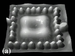
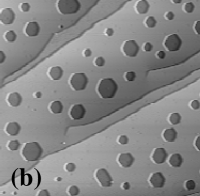
Figure 1: Nanoscale electron resonators used in lifetime studies. (a) Pseudo three-dimensional representation of a constant current STM image of a rectangular corral approximately 9 nm $\times$ 10 nm constructed from 28 Mn atoms on Ag(111). In order to enhance the atomic structure the intensity is plotted on a logarithmic scale. The standing wave pattern inside is due to electron confinement kli00_ . (b) Greyscale representation of a constant-current STM image of a 240 nm $\times$ 240 nm region of a Ag(111) surface showing numerous hexagonal monatomic vacancy islands. Surface state electrons are confined within these islands by strong scattering at the step edges of the vacancies.

results in energy quantisation, inducing spectral structure in the form of a series of resonant levels at energies that can be controlled through hanges in the dimensions and geometry of the resonator. The quasiparticle lifetime is then reflected in the level widths cra96_ ; kli01_ , but additional contributions arise due to lossy boundary scattering that must be accounted for if lineshape analysis is to be used to determine the intrinsic quasiparticle lifetime. In this paper we provide analytic and numerical results for the linewidths of electrons confined by different nanoscale resonators, and discuss their use in lifetime studies using STS.

The starting point of our analyses is the equation satisfied by the single particle Green function $G({\bf r},{\bf r}^{\prime})$ economou

$$\left(\!-\frac{\hbar^{2}\nabla^{2}}{2m^{\ast}}\!+\!V\!-\!E\!+\!i\text{Im}\,\Sigma_{\text{I}}\!\right)G({\bf r},{\bf r}^{\prime})\!=\!-\delta({\bf r}\!-\!{\bf r}^{\prime})$$ (1)

where ${\bf r}$ is a two-dimensional position vector, $m^{\ast}$ the effective mass and $E$ the electron energy with respect to the surface state band minimum. Confinement is due to the potential $V$, which in general will remain unspecified. Only the scattering properties of $V$ are relevant. We also include an inelastic potential or self energy $i\text{Im}\,\Sigma_{\text{I}}(E)$ to account for the effects of $e$-$e$ and $e$-$p$ scattering. This is related to the lifetime $\tau_{\,\text{I}}$ associated with these processes by $\tau_{\,\text{I}}=-\hbar/(2\text{Im}\,\Sigma_{\text{I}})$. ech04_ The local density of surface states (LDOS) is obtained from the Green function as $\rho({\bf r};E)=-(2/\pi)\text{Im}G({\bf r},{\bf r})$ (the 2 is for spin-degeneracy). We associate the LDOS with $dI/dV$ in the usual way ter85_ . In section II we consider circular atomic corral resonators, and in section III circular adatom and vacancy islands. Non-circular resonators are discussed in section IV. Contributions to experimentally measured linewidths arising from thermal broadening and instrumental effects are described in section V, and in section VI we illustrate how the results of our analyses may be used to identify appropriate resonator structures for lifetime studies.

II Atomic corrals

Atomic corrals are artificial structures in which individual adatoms are positioned with atomic scale precision into closed geometries cro93b ; kli00b ; kli01_ ; bra02_ . Strong scattering of the surface state electrons by the surrounding adatoms leads to confinement. The “standard model” for describing these systems is the $s$-wave scattering model hel94_ , in which the solution to (1) is given by hel94_ ; kli01_

$$\!\!\!\!\!\!\!\!\!G({\bm{r}},{\bm{r}}^{\prime}) \!=\! G_{0}({\bm{r}},{\bm{r}}^{\prime})\!+\!\sum_{j,k}G_{0}({\bm{r}},{\bm{R}}_{j})T^{jk}G_{0}({\bm{R}}_{k},{\bm{r}}^{\prime})$$ (2a)

$$T^{jk} \!=\! t\delta_{jk}+t\sum_{l\neq j}G_{0}({\bm{R}}_{j},{\bm{R}}_{l})T^{lk}.$$ (2b)

The sums in (2) are over the $N$ identical adatoms at locations ${\bf R}_{j}$, $j=0,1,..N-1$, which are characterised by the scattering $t$-matrix $t=(i/m^{\ast})(\exp 2i\delta-1)$, where $\delta$ is the phaseshift. $G_{0}$ denotes the free-electron propagator economou

$$G_{0}({\bm{r}},{\bm{r}}^{\prime})=-\frac{im^{\ast}}{2\hbar^{2}}H_{0}^{(1)}(\kappa|{\bm{r}}-{\bm{r}}^{\prime}|)$$ (3)

where $H_{0}^{(1)}$ is a Hankel function of the first kind abram and $\kappa=\sqrt{2m^{\ast}(E-i\text{Im}\Sigma_{\text{I}})/\hbar^{2}}$. In the case of a circular corral, and taking ${\bf R}_{j}=S(\cos\vartheta_{j},\sin\vartheta_{j})$, $\vartheta_{j}=2\pi j/N$, when both ${\bf r}$ and ${\bf r}^{\prime}$ are at the center of the corral

$$G-G_{0}=\left(-\frac{im^{\ast}}{2\hbar^{2}}H_{0}^{(1)}(\kappa S)\right)^{2}\frac{N}{t^{-1}-{\cal G}}$$ (4)

and the LDOS at the corral center is

$$\rho=\rho_{0}+\frac{2N}{\pi}\left(\frac{m^{\ast}}{2\hbar^{2}}\right)^{2}\text{Im}\frac{[H_{0}^{(1)}(\kappa S)]^{2}}{t^{-1}-{\cal G}}$$ (5)

where $\rho_{0}=(m^{\ast}/\pi\hbar^{2})(1\!-\!(2/\pi)\arg\kappa)$ is the clean surface LDOS jli98c and

$${\cal G} = -\frac{im^{\ast}}{2\hbar^{2}}\sum_{j=1}^{N-1}H_{0}^{(1)}(\kappa|{\bf R}_{j}-{\bf R}_{0}|)$$ (6a)

$$\approx -\frac{im^{\ast}}{2\hbar^{2}}\left[NJ_{0}(\kappa S)H_{0}^{(1)}(\kappa S)-{\cal C}\right].$$ (6b)

The last result follows using $|{\bf R}_{j}-{\bf R}_{0}|=2S\sin\vartheta_{j}/2$ and replacing the sum by an integral over $\pi/N\leq\vartheta\leq 2\pi-\pi/N$. $J_{0}$ is a Bessel function abram and ${\cal C}=1+(2i/\pi)(\ln(\kappa/4\mu)+\gamma-1)$, with $\gamma=0.57721\ 56649...$ (Euler’s constant). We have introduced $\mu=N/2\pi S$, the linear density of atoms making up the corral. Poles in the Green function which correspond to bound electron states that have amplitude at the center of the corral occur when $t^{-1}={\cal G}$. Using the asymptotic forms abram for $J_{0}$, $H_{0}^{(1)}$ gives the condition as

$$e^{2i\kappa S-i\pi/2}+1=\Omega(\kappa)$$ (7a)

$$\Omega(\kappa)=\frac{\kappa}{2\mu}\left[{\cal C}+\left(-\frac{im^{\ast}t}{2\hbar^{2}}\right)^{-1}\right].$$ (7b)

In the limit $\mu\rightarrow\infty$ the solutions to (7) are when $\kappa=\kappa_{n}=(n\pi-\pi/4)/S$, corresponding to a series of resonances at energies

$$E_{n}=\frac{\hbar^{2}(n\pi-\pi/4)^{2}}{2m^{\ast}S^{2}}$$ (8)

and with widths (full width at half maximum)

$$\Gamma_{\text{I}n}=-2\text{Im}\Sigma_{I}(E_{n})=\hbar/\tau_{I}(E_{n}).$$ (9)

This is the “hard-wall” limit, where the surface state wavefunction vanishes at the radius of the corral. cro93b The exact energies in this limit have the same form as (8) but with $(n\pi-\pi/4)$ ($=2.36,5.50,8.64$ for $n\!=\!1,2,3$ ) replaced by the n’th zero abram of the Bessel function $J_{0}$, $j_{0,n}$ ($=2.40,5.52,8.65$ for $n=1,2,3$). This close agreement validates the use of asymptotic forms in obtaining (7).

In the hard-wall limit (9) shows that the resonance widths are directly related to the inelastic $e$-$e$ and $e$-$p$ scattering rates at the energy of the level. However, in practice there are physical limits to how large the linear adatom density $\mu$ can become, with $\mu\leq d_{\text{nn}}^{-1}$ where $d_{\text{nn}}$ is the nearest-neighbour separation of surface atoms. Consequently the confinement is always less effective than in the hard-wall limit, which results in increased level widths. Solving (7) to first order in this case yields level widths

$$\Gamma_{n}=\Gamma_{\text{I}n}+\Gamma_{\text{C}n}$$ (10)

where

$$\Gamma_{\text{C}n}\approx\frac{\hbar^{2}\kappa_{n}}{m^{\ast}S}\text{Re}\ln\left[1-\Omega(\kappa_{n})\right].$$ (11)

This is the contribution to the level widths due to lossy scattering by the corral adatoms. Figure 2 shows the typical behaviour of $\Gamma_{\text{C}}$, showing results

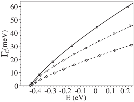
Figure 2: Calculated level widths for Fe corrals on Cu(111) using $\text{Im}\Sigma_{\text{I}}\!=\!0,m^{\ast}\!=\!0.38\,m_{\text{e}},im^{\ast}t\!=\!1,E_{0}\!=\!-0.44$ eV. hel94_ Squares and lozenges denote values found solving (7) by Newton-Raphson iteration for $N=48,S=71.3$ Å and $N=96,S=142.6$ Å respectively. Circles denote values found by non-linear least-square fitting of a series of Lorenzians to the LDOS given by (5) for $N=48,S=142.6$ Å. The lines are plots of $(\hbar^{2}\kappa/m^{\ast}S){\text{Re}}\ln[1-\Omega(\kappa)]$, $\kappa=\sqrt{2m^{\ast}(E-E_{0})/\hbar^{2}}$ for the respective corral parameters.

for Fe corrals on Cu(111) of various sizes and linear adatom densities. The accuracy of the approximations made in obtaining the expression in (11) are confirmed by the close agreement to be found between the level widths predicted by it and with those found by fitting the LDOS (5) with a series of Lorenzians or from iterative solution to (7). The general trend to be observed in the level widths is that they ncrease almost linearly with energy but are approximately halved by simultanously doubling the radius and the number of atoms in the boundary ring.

III adatom and vacancy islands

In a second class of resonator confinement results from scattering at ascending or descending steps. These are adatom or vacancy islands. avo94_ ; jli98b ; jli99_ ; jen04_ In these systems the scattering properties of the confining step are conveniently characterised by a reflection coefficient $R$. bur98_

Assuming circular symmetry, with $S$ now the island radius, the Green function can be expanded as

$$G({\bf r},{\bf r}^{\prime};E)=\frac{1}{2\pi}\sum_{M}G_{M}(\varrho,\varrho^{\prime};E)e^{iM(\varphi-\varphi^{\prime})}.$$ (12)

Substituting in to (1) gives for $\varrho,\varrho^{\prime}<S$

$$\varrho^{2}\frac{\partial^{2}G_{M}}{\partial\varrho^{2}}+\varrho\frac{\partial G_{M}}{\partial\varrho}+(\kappa^{2}\varrho^{2}-M^{2})G_{M}=\frac{2m^{\ast}}{\hbar^{2}}\varrho\ \delta(\varrho-\varrho^{\prime}).$$ (13)

Solving by the direct method gives for $\varrho<\varrho^{\prime}<S$

$$G_{M}(\varrho,\varrho^{\prime};E)=\frac{i\pi m^{\ast}}{\hbar^{2}\left[A_{M}-1\right]}J_{M}(\kappa\varrho)\Psi_{M}(\kappa\varrho^{\prime})$$ (14)

where $J_{M}$ is a Bessel function and $\Psi_{M}(z)=H^{(1)}_{M}(z)+A_{M}H^{(2)}_{M}(z)$, a linear combination of Hankel functions. The coefficient $A_{M}$ is chosen to ensure that $\Psi_{M}$ satisfies the scattering boundary conditions at $S$.

Identifying the energy levels from the poles in the Green function, we see from (14) that these arise whenever $A_{M}=1$. Only circularly symmetric states contribute to the local density of states at the center of the island ($J_{M}(0)=0$ for $M\neq 0$) so that the energy levels that can be seen by STS measurements at the center of islands occur when $A_{0}=1$. Using the asymptotic forms for the Hankel functions

$$\Psi_{0}(\kappa\varrho) \sim \sqrt{\frac{2}{\pi\kappa\varrho}}\left[e^{i(\kappa\varrho-\pi/4)}+A_{0}e^{-i(\kappa\varrho-\pi/4)}\right]$$ (15)

$$\propto \left[e^{i\kappa(\varrho-S)}+Re^{-i\kappa(\varrho-S)}\right],$$

that is, one can recognise within $\Psi_{0}$ waves incident and reflected from the confining potential, enabling the coefficient $A_{0}$ to be related to the planar reflection coefficient $R$ of the step at the island edge. Using this relationship and equating $A_{0}$ to 1 gives

$$Re^{2i\kappa S}e^{-i\pi/2}-1=0$$ (16)

as the condition for bound states visible in STS at the center of islands. Assuming confinement sufficient to give an identifiable series of resonant levels, and writing $R=|R|\exp i\phi_{R}$, (16) predicts their energies as

$$E_{n}=\frac{\hbar^{2}(n\pi+\pi/4-\phi_{R}/2)^{2}}{2m^{\ast}S^{2}}$$ (17)

and corresponding widths

$$\Gamma_{n}=\Gamma_{\text{I}n}+\Gamma_{\text{R}n}$$ (18)

where

$$\Gamma_{\text{R}n}\approx-\frac{\hbar^{2}}{m^{\ast}}\sqrt{\frac{2m^{\ast}E_{n}}{\hbar^{2}}}\frac{\ln|R|}{S}$$ (19)

The “hard-wall” limit in this case is $R\rightarrow-1$, which ensures that the wavefunction (15) vanishes at $S$. In this limit (17) coincides with (8) and $\Gamma_{\text{R}n}=0$ so that once again the resonance widths are directly related to the inelastic $e$-$e$ and $e$-$p$ scattering rates.

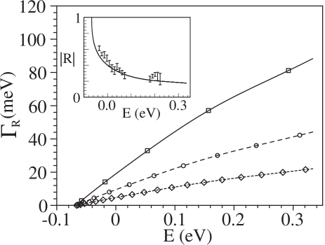
Figure 3: Calculated level widths for circular Ag vacancy islands using $\text{Im}\Sigma_{I}=0$, $m^{\ast}=0.42$, and $E_{0}=-67$ meV, for island radii 75 Å(squares), 150 Å(circles), and 300 Å(lozenges). The lines are plots of $-(\hbar^{2}/m^{\ast}S)\sqrt{2m^{\ast}(E-E_{0})/\hbar^{2}}\ln|R|$ for the respective island radii. The inset shows the reflection coefficient used in the calculation (line), along with the experimental values from Ref. [bur98_, ].

In reality, scattering at real steps has been found to be lossy, so that $|R|<1$, and then (19) enables to be estimated the resulting additional contribution to the level width $\Gamma_{\text{R}}$. Figure 3 shows widths found by solving (16) for variously sized Ag vacancy islands using an energy-dependent step reflection coefficient fitted to experimentally determined values bur98_ , along with the widths expected using the approximate expression (19). The agreement is again very good. The widths show similar behaviour to those in the atomic corrals, increasing approximately linearly with energy and inversely proportional to the island radius.

IV non-circular resonators

Equations (11) and (19) enable the ready determination of the lossy scattering contribution to the spectral linewidths of electron states in circular resonators. In terms of lifetime studies, circular resonators have two distinct advantages. Firstly, the high symmetry results in the sparsest spectrum, which simplifies the extraction of linewidths. This point is discussed more fully below. Secondly, it is not generally possible to obtain an analytic expression for the spectral linewidths in the case of non-circular resonators. Nevertheless, non-circular resonators are important, for example the atomic structure of the (111) surfaces favours the natural formation of triangular and hexagonal resonators.

Figure 4 shows the calculated linewidths due to lossy boundary scattering of electron

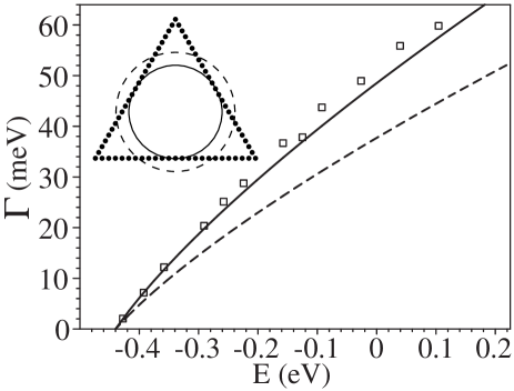
Figure 4: Calculated level widths (squares) found by non-linear least-squares fitting of a series of Lorenzians to the local density of states at the center of a triangular corral, side 220.5 Å constructed from 72 Fe atoms on Cu(111) (the structure reported in Ref. [cro95_, ]). Calculation parameters: $\text{Im}\Sigma_{I}=0$, $m^{\ast}=0.38$, $im^{\ast}t=1$, $E_{0}=-0.44$ eV. The lines are plots of the circular corral linewidth relationship, equation (11), for: dashed line, radius 81.9 Å; and solid line, radius 63.7 Å. The inset shows the atomic structure of the triangular corral, and the size of the two circles.

states with amplitude at the center of a 72 Fe atom triangular corral on Cu(111), side $d=220.5$ Å. An analytic treatment for this geometry is not possible, and so these widths have been obtained by fitting a series of Lorenzians to the local density of states which is obtained by numerically evaluating the Green function using equations 2a,2b. The resonant levels occur at energies that are close to those of the hard wall limit, $E_{p,q}=8\pi^{2}\hbar^{2}(p^{2}+q^{2}+pq)/(3m^{\ast}d^{2})$ where $p=1,2,3,\dots$, $0\leq q\leq p-1$, and $p-q\neq 3\ \times$ integer.wli85_ Also shown in the figure is the linewidth relation (equation (11)) for circular corrals with radii $S=81.9$ Å, corresponding to the same area as the triangular corral, and $S=63.7$ Å, corresponding to the largest enclosed circle. In each case in evaluating (7b) we have used for $\mu$, the linear density of corral atoms, the value from the actual triangular corral, $\mu=72/(3d)$. The widths in the same-area circular corral underestimate the triangular corral widths by some $\approx 25\%$, but those for the inscribed circular corral provide a good description. Calculations on other hexagonal and rectangular resonators confirm this result. The lossy scattering contribution to the level widths at the center of non-circular resonators are approximately given by the appropriate circular resonator width relation (11) or (19), using for the radius that of the largest enclosed circle. Therefore when designing potential resonator structures for lifetime studies, lossy-boundary scattering effects can be estimated using these expressions, although more detailed calculations taking into account the actual geometry are needed for subsequent quantitative analysis of experimental spectra.

V Thermal and instrumental effects

For completeness, we note that in addition to the lossy-scattering contribution, the experimental linewidth also includes contributions due to instrumental and thermal effects. These must also be borne in mind when considering the use of resonators for lifetime determinations. The thermal broadening is induced by the temperature dependence of the Fermi-Dirac distribution function,ter85_ which enters via the requirement that electrons tunnel in STS from occupied states in the tip/sample to unoccupied states in the sample/tip. The effect on the differential conductivity is to convolute with the derivative of the Fermi-Dirac distribution,

$$\chi_{T}(V)=\chi_{T}(0)\cosh^{-2}(\text{e}V/2\text{k}T).$$ (20)

The thermal broadening function shown in Figure 5

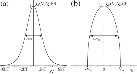
Figure 5: (a) Thermal broadening function, resulting from the temperature dependence of the occupation of electron states. (b) Instrumental broadening associated with the use of a modulating voltage and lock-in technique for recording the differential conductivity.

has a FWHM of $3.5\text{k}T$. This is a relatively small contribution at low temperatures (=$1.5\,\text{mV}$ at $T=10\,\text{K}$).

The differential conductivity is normally measured using a lock-in technique, which reduces phase-incoherent noise contributions. jkl_73 A sinusoidal voltage modulation $V_{\text{m}}\cos(\omega t)$ is superimposed upon the tunneling voltage $V$, and the signal at frequency $\omega$ recorded:

$$I_{\omega}(V) = \frac{2\omega}{\pi V_{\text{m}}}\int_{0}^{\pi/\omega}I(V+V_{\text{m}}\cos\omega t)\cos\omega t\,dt$$ (21)

$$= \int_{-\infty}^{\infty}\frac{dI}{dV}(V+V^{\prime})\chi_{\text{m}}(V^{\prime})\,dV^{\prime}.$$

The measured voltage is the differential conductivity convoluted with the instrumental function $\chi_{\text{m}}$,

$$\chi_{\text{m}}(V)=\left\{\begin{array}[]{ll}2\sqrt{V_{\text{m}}^{2}-V^{2}}/\pi V_{\text{m}}^{2}&\left|V\right|\leq V_{\text{m}}\\ 0&\left|V\right|>V_{\text{m}}.\end{array}\right.$$ (22)

The FWHM of this instrumental broadening function $\chi_{\text{m}}$, shown in Figure 5, is $1.7V_{\text{m}}$.

VI discussion

The results of the previous sections permit the design and use of resonator structures for the measurement of intrinsic lifetimes. To illustrate this, we consider circular atomic corrals constructed from

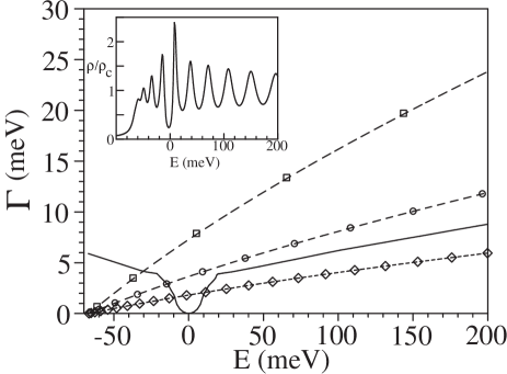
Figure 6: Linewidth contributions to states at the center of circular Ag adatom corrals on Ag(111). Intrinsic width due to $e$-$e$ and $e$-$p$ scattering (solid line — compiled from theoretical values reported in Refs. [kli00a, ; vit03_, ; eig02_, ]). Lossy boundary scattering: 60 atoms corral, radius 100 Å(squares); 120 atoms, radius 200 Å(circles); 240 atoms, radius 300 Å(lozenges). Inset: the LDOS normalised by $\rho_{\text{C}}=m^{\ast}/\pi\hbar^{2}$ at the center of the 120 atom corral.

Ag adatoms on Ag(111), for which a scattering phaseshift $\delta=0.75+0.42i$ has been measured. bra02_ The basic idea is that resonators with different dimensions result in different series of energy levels, at energies given by (8) (or more accurately by numerically solving (7)). By choosing an appropriate radius $S$, levels can be positioned at specific energies $\epsilon=E_{n}$. Using STS to measure the corresponding level width $\Gamma$, equations (10) and (11) plus knowledge of the thermal and instrumental broadening effects (section V) may then be used to identify $\tau_{\text{I}}(\epsilon)=\hbar/\Gamma_{\text{I}n}$.

Figure 6 compares theoretical estimates for the intrinsic many-body widths of the Ag(111) Shockley surface state with the boundary-loss contributions $\Gamma_{\text{C}n}$ that arise in variously-sized circular corrals. For the smallest corral of radius $S=10$ nm $\Gamma_{\text{C}}$ (squares) is significantly greater than $\Gamma_{\text{I}}$ (solid line) for most energies. In practice this will make harder the accurate determination of $\Gamma_{\text{I}}$ and hence lifetimes $\tau_{I}$ ($=\hbar/\Gamma_{\text{I}}$) from STS-measured linewidths, which will be the sum of $\Gamma_{\text{I}}$ and $\Gamma_{\text{C}}$, plus the effects of the convolution with $\chi_{T}$ (20) and $\chi_{\text{m}}$ (22). In the 20 nm radius corral the intrinsic and boundary-loss linewidth contributions are comparable for most energies, making it a better candidate structure for intrinsic lifetime determinations. One might consider going further, noting that for a fixed linear density of atoms making up the corral, $\mu=N/(2\pi S)$, the linewidth $\Gamma_{\text{C}}$ decreases linearly with $S$, encouraging the use of corrals of even greater radius. For almost all energies the lossy-scattering contribution $\Gamma_{\text{C}}$ in the 30 nm corral shown in Fig. 6 is smaller than the intrinsic linewidth $\Gamma_{\text{I}}$. However, from (8) we see that the level spacings vary as $1/S^{2}$, decreasing with radius more rapidly than $\Gamma_{\text{C}}$, so that in larger corrals the resonances merge, and the levels lose their integrity. This is already apparent at low energies in the 20 nm corral. The LDOS for this case is presented in the inset in Fig. 6, and shows that the lowest two levels are only just separated. If typical thermal and instrumental broadenings are included, then the lowest level becomes an indiscernable shoulder. Hence lifetimes $\tau_{\text{I}}^{\text{Ag}}$ are best measured in Ag adatom corrals with radii up to $\sim 20$ nm, with smaller resonators used for lifetimes at energies towards the bottom of the band of surface states.

We conclude by summarising the main results of this work. We have derived analytic expressions for the contribution to the spectral linewidths of electronic states measured using scanning tunneling spectroscopy at the centre of circular atomic corrals and adatom and vacancy islands that arises due to lossy boundary-scattering. Correcting measured linewidths for these contributions as well as thermal and instrumental broadening effects enables intrinsic linetimes due to electron-electron and electron-phonon scattering to be determined. The expressions that we have obtained are straightforward to evaluate, and also provide an estimate of lossy-confinement effects in non-circular resonators where the relevant radius is that of the largest enclosed circle. Using our linewidth expressions it is possible to design resonator structures appropriate for lifetime studies.

References

- (1) P. M. Echenique, R. Berndt, E. V. Chulkov, Th. Fauster, A. Goldmann, and U. Höfer, Surf. Sci. Rep. 52, 219 (2004).
- (2) J. Kliewer, R. Berndt, E. V. Chulkov, V. M. Silkin, P. M. Echenique and S. Crampin, Science 288, 1399 (2000).
- (3) A. Eiguren et al., Phys. Rev. Lett. 88, 066805 (2002); A. Eiguren, B. Hellsing, E.V. Chulkov, and P.M. Echenique, Phys. Rev. B 67, 235423 (2003).
- (4) L. Bürgi, O. Jeandupeux, H. Brune, and K. Kern, Phys. Rev. Lett. 82, 4516 (1999); S. Crampin, J. Kröger, H. Jensen, and R. Berndt, cond-mat/0410542.
- (5) K.-F. Braun and K.-H. Rieder, Phys. Rev. Lett. 88, 096801 (2002).
- (6) J. Li, W.-D. Schneider, R. Berndt, O. R. Bryant and S. Crampin, Phys. Rev. Lett. 81, 4464 (1998).
- (7) F. Reinert, G. Nicolay, S. Schmidt, D. Ehm and S. Hüfner, Phys. Rev. B 63, 115415 (2001).
- (8) J. Kliewer, PhD Thesis, RWTH Aachen (2000).
- (9) S. Crampin and O. R. Bryant, Phys. Rev. B 54, R17367 (1996).
- (10) J. Kliewer, S. Crampin, and R. Berndt, New J. Phys. 3, 22 (2001).
- (11) E. N. Economou, Green’s Functions for Quantum Physics (Springer-Verlag, Berlin, 1983).
- (12) J. Tersoff and D. R. Hamann, Phys. Rev. B 31, 805 (1985).
- (13) M. F. Crommie, C. P. Lutz, and D. M. Eigler, Science 262, 218 (1993).
- (14) J. Kliewer, R. Berndt, and S. Crampin, Phys. Rev. Lett. 85, 4936 (2000).
- (15) E. J. Heller, M. F. Crommie, C. P. Lutz, and D. M. Eigler, Nature (London) 369, 464 (1994).
- (16) M. Abramowitz and I. A. Stegun, Handbook of Mathematical Functions, (Dover, New York, 1972).
- (17) Ph. Avouris and L.-W. Lyo, Science 264, 942 (1994).
- (18) J. Li, W.-D. Schneider, R. Berndt, and S. Crampin, Phys. Rev. Lett. 80, 3332 (1998).
- (19) J. Li, W.-D. Schneider, S. Crampin, and R. Berndt, Surf. Sci. 422, 95 (1999).
- (20) H. Jensen, J. Kröger, R. Berndt, and S. Crampin, cond-mat/0411030.
- (21) L. Bürgi, O. Jeandupeux, A. Hirstein, H. Brune, and K. Kern, Phys. Rev. Lett. 81, 5370 (1998).
- (22) M. F. Crommie, C. P. Lutz, D. M. Eigler, and E. J. Heller, Physica D 83, 98 (1995).
- (23) W.K. Li and S. M. Blinder, J. Math. Phys. 26 2784 (1985).
- (24) J. Klein, A. Léger, M. Belin, D. Défourneau, M. J. L. Sangster, Phys. Rev. B 7, 2336 (1973).
- (25) L. Vitali, P. Wahl, M. A. Schneider, K. Kern, V. M. Silkin, E. V. Chulkov, and P. M. Echenique, Surf. Sci. 523, L47 (2003).