Conductance distribution in strongly disordered mesoscopic systems in three dimensions

Abstract

Recent numerical simulations have shown that the distribution of conductances $P(g)$ in three dimensional strongly localized systems differs significantly from the expected log normal distribution. To understand the origin of this difference analytically, we use a generalized Dorokhov-Mello-Pereyra-Kumar (DMPK) equation for the joint probability distribution of the transmission eigenvalues which includes a phenomenological (disorder and dimensionality dependent) matrix $K$ containing certain correlations of the transfer matrices. We first of all examine the assumptions made in the derivation of the generalized DMPK equation and find that to a good approximation they remain valid in three dimensions (3D). We then evaluate the matrix $K$ numerically for various strengths of disorder and various system sizes. In the strong disorder limit we find that $K$ can be described by a simple model which, for a cubic system, depends on a single parameter. We use this phenomenological model to analytically evaluate the full distribution $P(g)$ for Anderson insulators in 3D. The analytic results allow us to develop an intuitive understanding of the entire distribution, which differs qualitatively from the log-normal distribution of a Q1D wire. We also show that our method could be applicable in the critical regime of the Anderson transition.

I Introduction

The full distribution of conductances $P(g)$ for non-interacting electrons at zero temperature has recently been studied in detail in quasi one dimension (Q1D) both analytically mu-wo-go-03 and numerically pichard-nato ; q1dnumerics . Large mesoscopic fluctuations lead to several remarkable features in the distribution, including a highly asymmetric ‘one-sided’ log-normal distribution at intermediate disorder between the metallic and insulating limits mu-wo-99 ; go-mu-wo-02 , and a singularity in the distribution near the dimensionless conductance $g\sim 1$ in the insulating regime mu-wo-ga-go-03 . While some numerical studies exist for 3D finite size systems MK-PM ; markos1 ; SMO ; markos2 ; 3dnumerics , there is no analytic method currently available to study the full distribution $P(g)$ in 3D, especially at strong disorder. Theoretical work based on $2+\epsilon$ dimensions ($\epsilon\ll 1$), where a weak disorder approximation can be applied, has been used to propose that the critical distribution at the Anderson transition point has a Gaussian center with power law tails altshuler ; shapiro , but this can not be compared with numerical results in 3D MK-PM ; markos1 that show a highly non-trivial asymmetric distribution similar to the one-sided log-normal form of Q1D. It has not been possible so far to study analytically even the simpler case of $P(g)$ in the deeply insulating regime in 3D, where numerical results point to non-trivial deviations from the expected log-normal form markos2 .

The $P(g)$ in Q1D systems were studied analytically within the transfer matrix approach pichard-nato . In this paper we use a recently proposed generalization of the Q1D approach mu-go-02 to obtain analytically for the first time the full $P(g)$ for strongly disordered 3D systems. A brief account of the work has been published earlier mmwk . In Sections II and III we review briefly the DMPK equation and its generalization, respectively. In Sect. IV we analyze in detail the numerical data for 3D disordered systems in all three transport regimes: metallic, insulating and critical. Numerical data allow us to determine the free parameters of a matrix $K$ which appears in the generalized DMPK equation. In Sect V we use them to formulate a simple model for $K$, and solve the generalized DMPK equation analytically. In Sect. VI, an analytical formula for the conductance distribution $P(g)$ is derived in detail. In our model, the form of $P(g)$ is determined by two parameters, $\Gamma$, which measures the strength of the disorder, and $\gamma_{12}$, which determines the strength of the interaction term in the generalized DMPK equation. $\gamma_{12}\equiv 1$ in the Q1D systems. The fact that $\gamma_{12}<1$ in 3D makes the statistics of the conductance in 3D different from that in Q1D. Although we introduced two new disorder dependent parameters, they turn out to be related to each other and we show that the present model is not in contradiction with the single parameter scaling theory AALR . In Sect. VII we compare the analytical formula for the conductance distribution with the numerical data and analyze how the distribution $P(\ln g)$ depends on the parameter $\gamma_{12}$. In the limit $\gamma_{12}\to 1$, we recover the Q1D results. Sect. VIII discusses the possible extension of our solution to the critical point. We show that our results describe the critical regime qualitatively correctly, including the non - analyticity of the critical conductance distribution. Finally, summary and conclusions are given in Sect. IX.

II The transfer matrix approach

The distribution of conductances for non-interacting electrons at zero temperature can be studied within the transfer matrix approach. In this approach, a conductor of length $L_{z}$ and cross-section $L\times L$ is placed between two perfect leads; the scattering states at the Fermi energy then define $N\propto L^{2}$ channels. The $2N\times 2N$ transfer matrix $M$ relates the flux amplitudes on the right of the system to those on the left muttalib . Flux conservation and time reversal symmetry (we consider the case of unbroken time reversal symmetry only) restricts the number of independent parameters of $M$ to $N(2N+1)$ and $M$ can be written in general as dmpk ; muttalib

$$M=\left(\matrix{u&0\cr 0&{u}^{*}\cr}\right)\left(\matrix{\sqrt{1+\lambda}&\sqrt{\lambda}\cr\sqrt{\lambda}&\sqrt{1+\lambda}\cr}\right)\left(\matrix{v&0\cr 0&{v}^{*}\cr}\right),$$ (1)

where $u,v$ are $N\times N$ unitary matrices, and $\lambda$ is a diagonal matrix, with positive elements $\lambda_{i},i=1,2,...N$. Microscopic distribution of impurities will lead to a distribution $p_{L_{z}}(M)d\mu(M)$ of the transfer matrices where $d\mu(M)$ is an invariant measure which we rewrite as

$$p_{L_{z}}(M)d\mu(M)=p_{L_{z}}(\lambda,u,v)d\mu(\lambda)d\mu(u)d\mu(v).$$ (2)

If we know the marginal distribution

$$\bar{p}_{L_{z}}(\{\lambda_{a}\})=\int p_{L_{z}}(\lambda,u,v)d\mu(u)d\mu(v),$$ (3)

then the distribution of conductances $P(g)$ can be written as

$$P(g)=\int\cdots\int\prod_{a=1}^{N}d\lambda_{a}\bar{p}_{L_{z}}(\{\lambda_{a}\})\delta\left(g-\sum_{a=1}^{N}\frac{1}{1+\lambda_{a}}\right),$$ (4)

where

$$g=\sum_{a=1}^{N}\frac{1}{1+\lambda_{a}}$$ (5)

is the Landauer conductance landauer . A systematic approach to evaluate the $N$-dimensional integral, based on a mapping to a one-dimensional statistical mechanical problem, has been developed mu-wo-go-03 , so the full distribution $P(g)$ can be obtained if the marginal distribution $\bar{p}_{L_{z}}(\{\lambda_{a}\})$ is known. Note that the distribution of other transport variables which can be written as $\sum_{a}f(\{\lambda_{a}\})$, e.g. shot noise power blanter $P=\sum_{a=1}^{N}\frac{\lambda_{a}}{(1+\lambda_{a})^{2}}$ or conductance of N-S (Normal metal-Superconductor) microbridge beenakkerNS $G=\sum_{a=1}^{N}\frac{1}{(1+2\lambda_{a})^{2}}$, can also be obtained in the same way. The above approach is valid in principle for all strengths of disorder, in all dimensions.

If we assume that the distribution $p_{L_{z}}(\lambda,u,v)$ is independent of $u,v$, then the evolution of the distribution with length $L_{z}$ can be obtained from a Fokker-Planck equation first derived by Dorokhov and by Mello, Pereyra and Kumar dmpk which has become known as the DMPK equation:

$$\frac{\partial p_{L_{z}}(\lambda)}{\partial(L_{z}/\ell)} = \frac{2}{N+1}\frac{1}{J}\sum_{a}^{N}\frac{\partial}{\partial\lambda_{a}}\left[\lambda_{a}(1+\lambda_{a})J\frac{\partial p}{\partial\lambda_{a}}\right],$$ (6)

$$J \equiv \prod_{a<b}^{N}|\lambda_{a}-\lambda_{b}|^{\beta}.$$ (7)

Here $\ell$ is the mean free path and the parameter $\beta$ is equal to $1,2$ or $4$ depending on orthogonal, unitary or symplectic symmetry of the transfer matrices. We will consider only the case with time-reversal symmetry, for which $\beta=1$. Although the parameters $\lambda_{a}$ are not eigenvalues of $M$, it turns out that they determine the eigenvalues of the matrix $TT^{\dagger}$ ($T$ is the transmission matrixPth )

$$TT^{\dagger}=v^{*}(1+\lambda)^{-1}v$$ (8)

which characterizes the conductance given by Eq. (5), and the matrix $v$ contains the eigenvectors of $TT^{\dagger}$. So we will loosely refer to these as the eigenvalues and the eigenvectors in the text. Note that the parameter $\beta$ determines the strength of ‘level repulsion’ between eigenvalues.

The assumption that $p_{L_{z}}(\lambda,u,v)$ is independent of $u,v$ restricts the validity of the DMPK equation to quasi one dimension (Q1D). Quasi 1D means not only that $L_{z}\gg L$ where $L_{z}$ is the direction of the current and $L$ is the cross-sectional dimension, but it also requires that $\xi\gg L$, where $\xi$ is the localization length. In this limit, all channels become ‘equivalent’, the matrices $u$ and $v$ become isotropic and the distribution becomes independent of $u$ or $v$. The distribution of conductances $P(g)$ for such Q1D systems has been studied recently; it has many surprising features arising from large mesoscopic fluctuations. These include a highly asymmetric ‘one-sided’ log-normal distribution at intermediate disorder between the metallic and insulating limits mu-wo-99 ; go-mu-wo-02 , and a singularity in the distribution near $g\sim 1$ in the insulating regime mu-wo-ga-go-03 . It is not clear if these features persist in higher dimensions.

III Generalized DMPK equation in higher dimensions

To study 3D systems, a phenomenological generalization of the DMPK equation has recently been proposed in which the Q1D restriction is lifted in favor of an unknown matrix

$$K_{ab}\equiv\left<k_{ab}\right>_{L};\;\;\;k_{ab}\equiv\sum_{\alpha=1}^{N}|v_{a\alpha}|^{2}|v_{b\alpha}|^{2},$$ (9)

where the angular bracket represents an ensemble average. In terms of this matrix, the marginal distribution $\bar{p}_{L_{z}}(\lambda)$ satisfies an evolution equation given by mu-go-02

$$\frac{\partial\bar{p}_{L_{z}}(\lambda)}{\partial(L_{z}/\ell)} = \frac{1}{\bar{J}}\sum_{a}^{N}\frac{\partial}{\partial\lambda_{a}}\left[\lambda_{a}(1+\lambda_{a})K_{aa}\bar{J}\frac{\partial\bar{p}}{\partial\lambda_{a}}\right],$$ (10)

$$\bar{J} \equiv \prod_{a<b}^{N}|\lambda_{a}-\lambda_{b}|^{\gamma_{ab}};\;\;\;\gamma_{ab}\equiv\frac{2K_{ab}}{K_{aa}}.$$ (11)

In Q1D under the isotropy condition, the matrix $K$ reduces to

$$K^{Q1D}_{ab}=\frac{1+\delta_{ab}}{N+1};\;\;\;\gamma^{Q1D}_{ab}=1,$$ (12)

and one recovers the DMPK equation (with $\beta=1$). In 3D, $K$ is not known analytically, and must be obtained from independent numerical studies.

There are two major assumptions made in Ref. [mu-go-02, ] in deriving Eq. (10):

• the elements $k_{ab}$ can be replaced by their mean values $K_{ab}$, and

• the $L_{z}$-dependence of $K_{ab}$ is negligible.

These assumptions need to be verified before the equation can be used. Note that the matrix $K$ depends on the choice of representation. Since the assumptions are most natural in the position representation, we will study the matrix in this representation.

IV Numerical data

The generalized DMPK equation apparently introduces a large number of new parameters, elements of the matrix $K_{ab}$. There is no theoretical prediction about how these parameters should depend on the size of the system or on disorder. We only know that in the Q1D limit they should follow Eq. (12). Therefore our first goal is to study numerically various 3D and Q1D systems systematically in detail in order to answer the following questions:

• Are the assumptions (i) and (ii) discussed in Section III valid at all strengths of disorder?

• How do the elements $K_{ab}$ depend on disorder and on the system size?

• How do the elements $K_{ab}$ depend on the indices $a$ and $b$?

• Given the size, disorder and index dependence of $K_{ab}$, is it possible to construct a simple model of $K$ at all disorder with only a small number of parameters?

We will address all of the above in this section, but let us first briefly discuss the numerical procedure used to evaluate $K$.

We consider the tight binding Anderson model defined by the Hamiltonian

$${\cal H}=W\sum_{n}\varepsilon_{n}c_{n}^{\dagger}c_{n}+\sum_{[nn^{\prime}]}t_{nn^{\prime}}c^{\dagger}_{n}c_{n^{\prime}}.$$ (13)

In Eq. (13), $n=(xyz)$ counts sites on the simple cubic lattice of the size $L\times L\times L_{z}$, and $\varepsilon_{n}$ are random energies, uniformly distributed in the interval $[-\frac{1}{2},\frac{1}{2}]$. The parameter $W$ measures the strength of disorder. The Fermi energy is chosen as $E_{F}=0.01$. The hopping term $t_{nn^{\prime}}$ between the nearest-neighbor sites $nn^{\prime}$ is unity for hopping along the $z$ direction and $t_{nn^{\prime}}=t$ for hopping in the $x$ and $y$ directions. Then the dispersion relation is

$$E=2\cos k_{z}+2t\cos k_{x}+2t\cos k_{y}$$ (14)

For a given cross section of the sample: $L_{x}=L_{y}=L$, $k_{x}$ and $k_{y}$ possess values $\pi/(L+1)\times 1,2,\dots L$ (we consider hard wall boundary conditions). At fixed energy E, given values of $k_{x}$ and $k_{y}$ determine the value of $k_{z}$, which is either real (if $|\cos k_{z}|<1$) or imaginary. The latter case corresponds to closed channels which do not transmit current in perfect leads. To avoid these closed channels, which are not considered in the DMPK formulation, we use $t=0.4$. Then the model Eq. (13) exhibits a metal-insulator transition zambetaki at $W_{c}\approx 9$. To obtain transport properties, we use the transfer matrix method of [pendry, ]. The main difference from previous works SMO ; markos2 is that we also calculate eigenvectors of the matrix $TT^{\dagger}$. Using Eq. (1), we calculate numerically the matrix $TT^{\dagger}$. Owing to Eq. (8), diagonalizing $TT^{\dagger}$ gives us $\lambda$ as well as all elements of the matrix $v$.

Note that the eigenvectors depend on the representation. In the original formulation of the DMPK approach, semi-infinite leads consist of mutually independent and equivalent 1D wires. Therefore, the transfer matrix in the leads is diagonal in both channel and space representations. In numerical work, we need to distinguish between these two, since the transfer matrix is diagonal only in the channel representation. We therefore calculate the matrix $TT^{\dagger}$ in the channel representation, find eigenvalues and eigenvectors, and transform the latter back to the space representation to obtain the matrix $v$. Elements of $v$ are then used for the calculation of the matrix $K$ in the space representation.

We now go back and address the questions raised at the beginning of this section.

IV.1 Q1: Validity of the assumptions (i) and (ii)

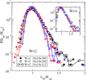
Figure 1: Probability distribution of normalized $k_{ab}$ for Q1D systems. ($\circ$: $a=b=1$, $\diamondsuit$: $a=1$, $b=2$, $\bigtriangledown$: $a=b=2$). Full symbols: $W=2$, $L=10$, $L_{z}=16L$; open symbols: $W=2$, $L=10$, $L_{z}=24L$. Lines with symbols: $W=2$, $L=14$, $L_{z}=8L$. Data confirm that the distribution becomes narrower when $L$ increases. Inset shows the same for $W=4$ and $L=18$, $L_{z}=4L$. As expected, distributions are broader.

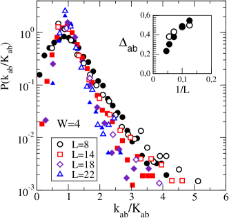
Figure 2: The distribution of normalized $k_{ab}$ for 3D systems with $W=4$ and various system sizes. (critical disorder $W_{c}\approx 9$.) Open symbols: $a=b=1$; full symbols: $a=1$, $b=2$. Inset shows the $L$-dependence of $\Delta_{ab}=\sqrt{\textrm{var}~{}k_{ab}}/K_{ab}$ which decreases when $L$ increases. Data confirm that distribution is self-averaging (it becomes narrower and $\Delta_{ab}\to 0$ when $L$ increases) although it is broader than in the Q1D case.

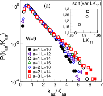
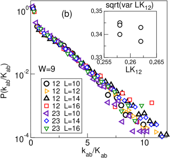
Figure 3: Probability distribution of normalized matrix elements $k_{ab}$. (a) $P(k_{aa}/K_{aa})$ ($a=1,2$ and 3) at the critical point $W=W_{c}\approx 9$. Distribution is $L$-independent (apart from the exponential tail which is broader for larger $L$ since mean value $K_{aa}\sim 1/L$). Note the logarithmic scale on the $y$ axis. (b) Distribution of off-diagonal elements $k_{12}$ and $k_{23}$ possess sharp maxima close to zero, and long exponential tails. Insets show standard deviations of distributions as a function of mean values for $8\leq L\leq 18$. These data also show the accuracy of our estimate of the critical point since we expect both the mean and the standard deviation to be $L$-independent at $W=W_{c}$. The distributions for Q1D systems $L\times L\times 8L$ are almost identical to those for cubes (data not shown).

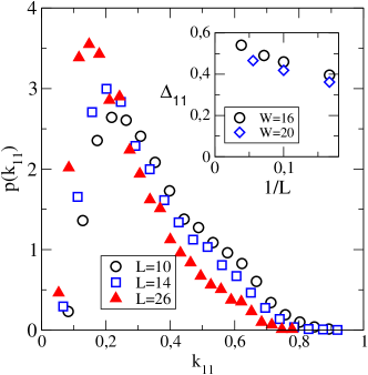
Figure 4: Probability distribution $P(k_{11})$ in the insulating regime ($W=16$). Although distribution becomes narrower when system size $L$ increases, it is not self-averaging. Inset shows the size dependence of the $\Delta_{11}=\sqrt{\textrm{var}~{}k_{11}}/K_{11}$ for $W=16$ and $W=20$. $\Delta_{11}$ converges to a non-zero constant when $L\to\infty$.

In order to check assumption (i), i.e. if the elements $k_{ab}$ can be replaced by their average $K_{ab}$ in 3D, we analyze the probability distribution $P(k_{ab})$. We start with the weakly disordered metallic regime. Two values of disorder were used: $W=2$ and $W=4$. More relevant than the actual strength of the disorder is the mean free path $\ell$ which can be estimated from the mean conductance pichard

$$\langle g\rangle=\frac{N}{L_{z}}\ell$$ (15)

with $N=L^{2}$. From the $L_{z}$ dependence of $\langle g\rangle$ in Q1D systems we estimate $\ell(W=2)\approx 9.2$ and $\ell(W=4)\approx 1.8$, in units of the lattice spacing.

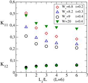
Figure 5: At the critical point, which depends on the anisotropy parameter $t$, both $LK_{11}$ and $LK_{12}$ converge to $L_{z}$-independent values when $L_{z}/L\to\infty$. The limiting value $LK_{11}$ depends on $t$. Shown are also data for the insulating regime $W=20$, $t=0.4$. All data for $K_{12}$ almost coincide so that they are not distinguishable in the figure.

First, we test how assumption (i) is fulfilled in the weakly disordered limit, where the DMPK equation is known to describe the universal features of transport statistics correctly. We show in Figure 1 the distribution $P(k_{ab})$ in the weakly disordered Q1D regime. As expected, the width of the distribution increases when $W$ increases, but $P(k_{ab})$ is self-averaging (it becomes narrower when $L$ increases). Figure 2 shows the same distribution for 3D systems. The distribution is again self-averaging, although much broader than in the Q1D case.

In the critical regime, the probability distribution $P(k_{ab})$ is no longer self-averaging but tends to be $L$-independent in the limit $L\to\infty$ (Fig. 3). Although the distributions possess long exponential tails, they have well defined sharp maxima, which do not depend on the system size.

In the insulating regime, the distribution $P(k_{11})$ becomes narrower when $L$ increases (Fig. 4). However, on the basis of our numerical data we conclude that the distribution is not self-averaging. Although var $k_{11}$ decreases when $L\to\infty$ (data not shown), the normalized width $\Delta_{11}=\sqrt{\textrm{var}~{}k_{11}}/K_{11}$ (shown in inset of fig. 4) slightly increases when $L$ increases. As $K_{11}$ itself is non-zero in the limit $L\to\infty$ (fig. 9), $\Delta_{11}$ should converge to an $L$-independent function for large $L$.

The distribution of off-diagonal elements $P(k_{12})$ in the insulating regime (not shown) is qualitatively the same as that at the critical point.

We conclude that both in the critical and localized regimes the distributions converge to $L$ independent functions with a well-defined peak, but the standard deviation is of the same order of magnitude as the mean. We note that the most-probable value of $k_{11}$ is always very close to its mean value; we therefore expect that replacing $k_{11}$ by its mean value $K_{11}$ is a reasonable approximation as long as one is interested in qualitative results only. Thus, although to leading order assumption (i) remains valid for all disorder, we have to keep in mind that fluctuations of the elements $k_{ab}$ in the strongly disordered regime might become important if the final results are sensitive to the exact values of these elements. We have checked that the final distribution of conductances do not change in any appreciable way if fluctuations of $k_{11}$ are included by overaging the conductance distribution over $P(k_{11})$.

To check assumption (ii), namely if the $L_{z}$ dependence of $K_{ab}$ is negligible, we studied the $L_{z}/L$ dependence of $K_{11}$ and $K_{12}$. Figure 5 confirms that for both critical and insulating regimes the parameters $K_{11}$ and $K_{12}$ converge to non-zero (although $t$ - dependent) limits when the length of the system increases. It shows that the properties of the matrix $K$ depend only slightly on the ratio $L_{z}/L$ and reach $L_{z}$-independent limiting values when $L_{z}/L\to\infty$ in all transport regimes. The assumption (ii) is therefore reasonably well satisfied at all disorder as long as $L_{z}\geq L$.

Thus we conclude from our numerical studies that to leading approximation the generalized DMPK equation (10) remains qualitatively valid at all disorder in 3D, but the effect of fluctuations of $k_{ab}$ on the final results has to be evaluated in more detail before a quantitative comparison with numerical results can be made.

IV.2 Q2: Disorder and size dependence of $K_{ab}$

We start with the weak disorder regime. To distinguish the generic $W$ dependence of $K_{11}$ from finite size effects, we analyzed in Fig. 6 the $L$ dependence of the parameter

$$\kappa=(N+1)K_{11}/2.$$ (16)

As expected, $\kappa$ decreases when $L$ increases. However, from the analysis of Q1D systems (also shown in Fig. 6) we conclude that $\kappa$ converges to 1 only for very small values of disorder. As shown in Fig. 6, $\kappa\approx 1.36$ for $W=4$. Thus, deviations from Eq. (12) already appear in the metallic limit, probably due to the decrease of the mean free path.

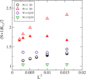
Figure 6: $1/L^{2}$ dependence of $\kappa=(N+1)K_{11}/2$ (open symbols) and $(N+1)K_{12}$ (full symbols) in the metallic regime. Data confirms that $\kappa$ depends on $L$. This agrees with data in Fig. 12. Also, $2K_{12}$ differs from $K_{11}$ for small $L$. This agrees with data in Fig. 13. To estimate limiting behavior of $K_{11}$, we also considered Q1D systems $L\times L\times 4L$. $\kappa$ is close to 1 only for very weak disorder $W=2$. For $W=4$ we obtained $\kappa\approx 1.36$. As this value does not depend on $L$ for $8\leq L\leq 18$ ($\Diamond$), we expect that 3D data for $W=4$ will converge to the same value when $L\to\infty$.

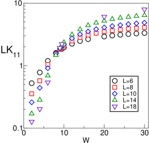
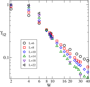
Figure 7: Disorder dependence of $K_{11}$ and $\gamma_{12}$ for various system sizes. Note the common crossing point at $W=W_{c}\approx 9$. Note also that $\gamma_{12}\to 1$ for $W<W_{c}$ and $L\to\infty$, as expected from DMPK, but $\gamma_{12}$ decreases with the system size for $W>W_{c}$.

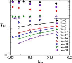
Figure 8: $\gamma_{12}$ as a function of the system size for various strengths of disorder. In the metallic regime, $\gamma_{12}$ converges to 1 when $L\to\infty$. At the critical point, $\gamma_{12}$ is $L$-independent, and in the insulating regime $\gamma_{12}$ decreases when $L$ increases. Solid lines are linear fits $\gamma_{12}=a+b/L$ with $a\sim 10^{-3}$ for $W\leq 40$.

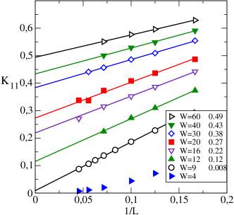
Figure 9: System size dependence of $K_{11}$ for various values of disorder. Solid lines are linear fits. Data in legend presents limiting values $\tilde{K}_{11}=\lim_{L\to\infty}K_{11}(L)$. Shown are also data for the metallic regime ($W=4$) for which $K_{11}\sim 1/L^{2}$ (Table I). While $\tilde{K}_{11}=0$ in metal and at the critical point ($W=9$), it is non-zero in the insulating regime. Thus, it may be used as the order parameter of the Anderson transition.

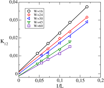
Figure 10: System size dependence of $K_{12}$ for various values of disorder in the insulating regime. Data confirm that $K_{12}\sim 1/L$ and that $\lim_{L\to\infty}K_{12}=0$.

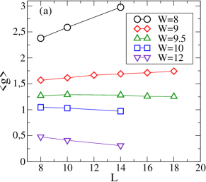
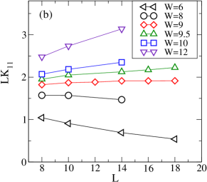
Figure 11: Estimation of the critical point from the mean conductance $\langle g\rangle$ and from $LK_{11}$. Both parameters $\langle g\rangle$ and $LK_{11}$ are $L$-independent at $W=W_{c}$. $LK_{11}\propto L$ ($\propto 1/L)$ in the insulating (metallic) regime, respectively. From data we conclude that $9<W_{c}<9.5$ and use $W_{c}=9$ throughout the paper.

In the next step we analyze how the matrix $K$ changes when the disorder increases. Typical results are given in Fig. 7. Our data show that the $L$ dependence of the parameters $LK_{11}$ and $\gamma_{12}$ is different for different transport regimes. While in the metallic regime $LK_{11}$ decreases as $\sim 1/L$ and $\gamma_{12}$ converges to unity when $L$ increases, qualitatively different behavior is obtained at strong disorder. In the insulating regime $K_{11}$ converges to a non-zero $L$-independent constant when $L\to\infty$ (Fig. 9) and $K_{12}$ converges to zero as $K_{12}\sim 1/L$ (Fig. 10). This means that $\gamma_{12}\sim 1/L$ in the insulating regime (Fig. 8).

Figures 7 a,b also show that there exists a critical disorder $W=W_{c}$ where both $LK_{11}$ and $\gamma_{12}$ are independent of $L$. Note that $\gamma_{12}<1$ at $W=W_{c}$. We found that the critical value $\gamma_{12c}$ depends on the anisotropy (Fig. 5). For the present case $t=0.4$, $\gamma_{12c}\approx 0.28$. The qualitative $L$ dependence in different transport regimes is summarized in Table 1.

disorder			$L\times{K_{11}}$			$\gamma_{12}$
$W\ll{W_{c}}$			$\sim L^{-1}$			1-${\cal{O}}(L^{-1})$
${W_{c}}$			const			const
$W\gg{W_{c}}$			$\sim L$			$\sim L^{-1}$

Table 1: Typical $L$-dependence of the parameters $K_{11}$ and $\gamma_{12}$ in the metallic, critical and localized regimes.

We observe that the disorder dependence of $K_{11}$ is consistent with $K_{11}\propto 1/L^{m}$, where $m=2,1,0$ in the metallic, critical and insulating limits, respectively, in agreement with Ref. [chalker, ]. Note that in contrast, $K_{11}\propto 1/L^{2}$ for all strengths of disorder in Q1D. This is a major difference between Q1D and 3D. One can understand qualitatively how the $L$ dependence of $K_{11}$ changes in the weak and strong disorder limits on general grounds. If all channels are equivalent, we expect the column matrix $v_{1a}\sim 1/\sqrt{N}$, which satisfies the unitary condition $\sum_{a=1}^{N}|v_{1a}|^{2}=1$. This leads to $K_{11}\sim 1/N=1/L^{2}$ in the metallic limit. On the other hand, if the localization length $\xi\sim 1$, then on any cross-section at a given $L_{z}$, we expect only a few sites on the back side of the sample to be ‘illuminated’ by an incoming wave, so we expect $v_{1a}\sim\delta_{1a}$. This leads to $K_{11}\sim 1$, independent of $L$. Similarly, since all $K_{1a}\propto 1/L^{2}$ in the metallic regime, we expect $\gamma_{12}\sim 1$ in the metallic regime. However, in the insulating regime, we have not found a simple physical argument why $K_{12}\propto 1/L$ and hence $\gamma_{12}\propto 1/L$. We also find numerically in the insulating regime that for $1\ll\xi\ll L$, $K_{11}\sim 1/\xi$. The structure of the eigenvector $v_{1a}$ that gives rise to $K_{11}\sim 1/\xi$ and $K_{12}\sim 1/L$ in the region $1\ll\xi\ll L$ is highly non-trivial, and deserves further study.

Figure 9 confirms our claim that $K_{11}>0$ in the insulating regime. Its limiting value, $\tilde{K}_{11}=\lim_{L\to\infty}K_{11}(L)$ can be used as an order parameter for the scaling analysis of the Anderson transition. It is evident that $\tilde{K}_{11}=0$ for $W<W_{c}$ and $\tilde{K}_{11}>0$ for $W>W_{c}$. We show in Fig. 11 the $L$-dependence of $LK_{11}$ and of the mean conductance $\langle g\rangle$ for various strengths of disorder. Similar behavior is shown in Fig. 8 for the parameter $\gamma_{12}$. One sees that all three parameters, $\langle g\rangle$, $LK_{11}$ and $\gamma_{12}$, could be used for the estimation of the critical disorder $W_{c}$, at which none of them depends on the system size.

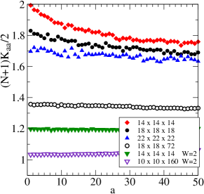
Figure 12: $a$-dependence of $K_{aa}\times(N+1)/2$ for 3D and Q1D systems with $W=2$, (mean free path $l\approx 9.2$) and for $W=4$ ($l\approx 1.8$). $K_{aa}$ are larger than is predicted by the DMPK theory. Good agreement with DMPK is observed only for Q1D systems with very small disorder ($W=2$).

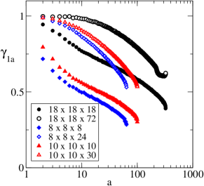
Figure 13: $a$-dependence of $\gamma_{1a}$ for the metallic regime ($W=4$). Finite size effects are clearly visible so that $\gamma_{12}=1$ only in the limit of large system size. As expected, convergence is better for Q1D systems than for cubes. Nevertheless, data confirm that $\gamma_{1a}$ converge to 1 in the limit $L\to\infty$ even when $K_{11}$ and $K_{12}$ do not converge to values assumed by DMPK given in Eq. (12).

IV.3 Q3: Index dependence of $K_{ab}$

Again we begin with weak disorder. To compare 3D and Q1D systems, we show in Fig. 12 the parameters $K_{aa}$ as a function of the index $a$. It is clear that the 3D data differ considerably from the DMPK value $2/(N+1)$. In Fig. 13 we show the ratio $\gamma_{1a}=2K_{1a}/K_{11}$ for various $L$ and compare it with Q1D numerical data. It is evident that $\gamma_{1a}$ converges to 1 when the system size increases, in spite of the fact that both $K_{1a}$ and $K_{11}$ differ from the DMPK values of Eq. 12. The convergence is much slower in 3D than in Q1D systems. Also, $\gamma_{1a}$ converges slower for larger $a$. We conclude that although 3D metals are qualitatively similar to Q1D metals, there are quantitative differences that need to be explored further.

In the critical regime, Figures 14 and 15 show that the $a$ and $b$ dependence of the matrix elements $K_{ab}$ can be described by simple functions: $K_{aa}\sim K_{11}/a^{1/2}$, $\gamma_{1a}\sim 1/La^{1/2}$. Although we did not analyze all matrix elements in detail, we believe that the data presented here support our expectation that all matrix elements $K_{ab}$ can be expressed in terms of $K_{11}$, $K_{12}$ and some simple function of the indices $a$ and $b$.

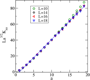
Figure 14: Critical point: We plot $La^{3/2}K_{aa}$ to show that $LK_{aa}\propto a^{-1/2}$ are $L$-independent for all $a\leq 20$

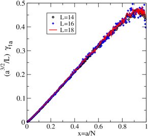
Figure 15: Critical point. From the linear dependence $(a^{3/2}/L)\gamma_{1a}\propto a/N$ we conclude that $\gamma_{1a}\propto 1/a^{1/2}L$. ($N=L^{2}$)

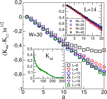
Figure 16: Insulating regime: $a$-dependence of $K_{aa}$ for 3D systems with $W=30$. To see the $a$-dependence more clearly, we plot the difference $[K_{aa}-K_{11}]\sqrt{a}$ which behaves as $\sim-a$ for small $a$. Solid line is a linear fit, from which we have $K_{aa}=K_{11}+0.05-0.04/\sqrt{a}$ for $L=18$ and $a\leq 18$ ($K_{11}=0.44$). Right inset presents data for $L=14$ and various strength of the disorder. Left inset shows $K_{aa}$ for $L=18$.

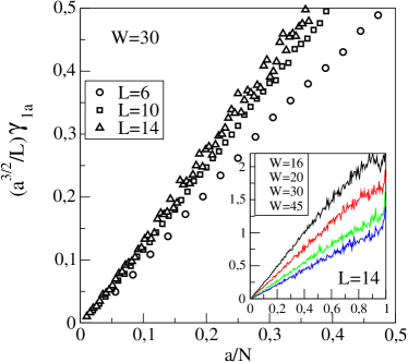
Figure 17: Insulating regime ($W=30$): $a$-dependence of $\gamma_{1a}$ ($L=6$, 10 and 14). Similar to the critical point, data shows that $a^{3/2}/L\times\gamma_{12}\sim a/N$ so that $\gamma_{1a}\sim 1/(\sqrt{a}L)$. Inset shows data for $L=14$ and various strength of the disorder.

In the insulating regime we find a simple $a$-dependence of the difference

$$K_{aa}-K_{11}\approx-c\sqrt{a}$$ (17)

with $|c|\sim 0.04$ (Fig. 16). We also found, (Fig. 17), that for $a<N/4$, $\gamma_{1a}\sim 1/\sqrt{a}L$, very close to the value obtained at the critical point note .

There is an interesting correspondence between the $a$-dependence of $K_{aa}$ and the $a$-dependence of the parameters $x_{a}$ defined through the parameters pichard-nato

$$\lambda_{a}=\sinh^{2}x_{a}$$ (18)

which is summarized in Table 2.

	metal	critical point	insulator
$x_{a}$	$ax_{1}$	$\sqrt{a}x_{1}$	$x_{1}+c\sqrt{a}$
$K_{aa}$	$K_{11}$	$K_{11}/\sqrt{a}$	$K_{11}-c/\sqrt{a}$

Table 2: Index dependence of $K_{aa}$ obtained in the present work compared to $x_{a}$ JPCM in the metallic, critical and insulating regimes.

We find that the index dependence of $K_{aa}$ can be ignored in the metallic regime. The $a$-dependence is more pronounced at the critical point and in the localized regime. On the other hand, higher channels ($a\gg 1$) do not contribute to the transport either at the critical point or in the localized regime, so the actual values of $K_{ab}$ for large $a$ and $b$ are not important. Therefore, we conclude that the weak index dependence of the matrix elements $K_{ab}$ is less relevant for transport properties compared to the dependence of the matrix elements on disorder in the $L\rightarrow\infty$ limit.

It is also worth mentioning that since we are interested only in $L$-independent quantities at the critical point, the $a$-dependence of any parameter is relevant only for $a\leq L$. When $a$ becomes comparable to $L$, we can not distinguish the true $a$-dependence from finite size effects.

IV.4 Q4: Simple model for K

Finally we ask the question if it is possible to construct a simple model of $K_{ab}$ with only a small number of independent parameters. We just concluded in the previous section that the weak index dependence of the matrix at strong disorder is not very important. We expect that the crude approximations

$$K_{aa}\approx K_{11}\;\;\;\textrm{and}\;\;\;\gamma_{ab}\approx\gamma_{12}$$ (19)

capture the major qualitative features of the matrix $K$.

Approximation (19) introduces two new parameters, $K_{11}$ and $\gamma_{12}$. We show that both parameters $K_{11}$ and $\gamma_{12}$ are unambiguous functions of the localization length. To do so, we calculated the limiting values of $K_{11}$ (Fig. 9) and of the parameter $x_{1}$ (Fig. 18) and plot $K_{11}$ versus $\xi$ (Fig. 19). We observe that the $\xi$ dependence of $K_{11}$ depends also on the anisotropy parameter $t$ (data not shown).

In the same way, we analyzed parameter $\gamma_{12}$. As was shown in Fig. 8, we expect $\gamma_{12}\sim L^{-1}$ in the localized regime. Data in Figures 9 and 10 support this assumption. To estimate the disorder dependence of $\gamma_{12}$, we plot in Fig. 20 the quantity

$$\lim_{L\to\infty}L\gamma_{12}=2L~{}\displaystyle{\frac{\lim_{L\to\infty}K_{12}}{\lim_{L\to\infty}K_{11}}}$$ (20)

which indeed increases linearly with localization length in the strongly localized regime.

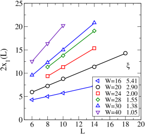
Figure 18: Insulating regime: Estimation of the localized length $\xi(W)$ from the linear $L$ dependence $x_{1}(L)=\textrm{const}+L/\xi$. ($\lambda_{1}=\sinh^{2}x_{1}$). Values of $\xi$ are given in the legend. $g\approx\cosh^{-2}x_{1}\approx\exp-2L/\xi$.

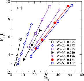
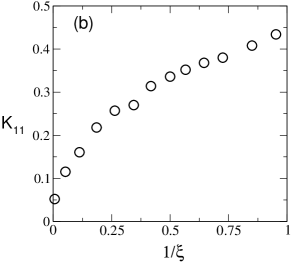
Figure 19: Figure (a) shows how $LK_{11}$ depends on $x_{1}$ for various disorder in the localized regime. Data confirm linear relation $LK_{11}\propto x_{1}$. Figure (b) shows how limiting values of $K_{11}$, obtained from the $L$-dependence of $K_{11}(L)$ (Fig. 9), depend on values of $1/\xi$ (Fig. 18). Data confirms that there is an unambiguous $\xi$-dependence of $K_{11}$.

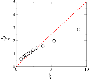
Figure 20: $L\gamma_{12}$ defined by Eq. (20) as a function of $\xi$. Data confirms that there is an unambiguous $\xi$-dependence of $\gamma_{12}$. This is important for the formulation of the single parameter scaling theory. Dashed line is the linear dependence $\gamma_{12}=\xi/2L$, considered in [mmwk, ].

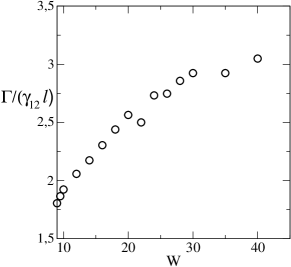
Figure 21: Ratio $\Gamma/(\gamma_{12}\ell)=1/2LK_{12}$, given by Eq. 23 for a cubic system, as a function of disorder for 3D systems in the insulating regime $W>W_{c}$.

V Solution of the generalized DMPK equation in the strong disorder limit

While modeling the full $\gamma_{ab}$ at the critical point needs more careful numerical studies, the insulating limit is simpler and provides a test case for the generalized DMPK equation (8). It predicts that the logarithmic interaction between the transmission eigenvalues $\lambda_{a}$ vanishes as $1/L$ in the insulating limit. In the rest of the paper we will test this prediction by evaluating the full distribution of conductances in the insulating limit for a 3D conductor as described by Eq. (8), using the simple approximate model for $K$ suggested by our numerical studies, namely

$$K_{aa}\approx K_{11}~{}~{}{\rm and}~{}~{}\gamma_{ab}\approx\gamma_{12}\sim\textrm{const.}\frac{\xi}{L}.$$ (21)

It is useful to introduce another parameter,

$$\Gamma=\frac{\ell}{L_{z}K_{11}}$$ (22)

and the ratio

$$\frac{\Gamma}{\gamma_{12}}=\frac{\ell}{L_{z}K_{11}\gamma_{12}}=\frac{L}{L_{z}}~{}\frac{\ell}{2LK_{12}}.$$ (23)

$\Gamma\sim 1/L_{z}\ll 1$ in the insulating regime, both in 3D ($L=L_{z}$) and Q1D ($L_{z}\gg L$) systems. It measures the strength of the disorder. The ratio $\Gamma/\gamma_{12}$ reduces to $\Gamma$ in the Q1D limit when $\gamma_{12}=1$. For 3D ($L_{z}=L$) we see in Fig. 21 that $\Gamma/\gamma_{12}\sim L\ell/L_{z}$ varies smoothly between about $2\ell$ and $3.5\ell$ when disorder increases from $W_{c}$ to infinity. Thus, the strength of disorder is characterized predominantly by the parameter $\Gamma$. For definiteness, we will use $\Gamma/\gamma_{12}=2$ appropriate for a cubic system when needed for comparison with numerical results noteG/g .

Note that fluctuations in $k_{aa}$, ignored in the model, would lead to fluctuations of $\Gamma$ and $\gamma_{12}$ as well, but will not change either the length or the disorder dependence of these parameters.

A brief description of the results has appeared in [mmwk, ]. Here we provide many of the details.

We rewrite the generalized DMPK as mu-go-02

$$\frac{\partial p_{s}(x)}{\partial(L_{z}/\ell)}=\frac{1}{4}\sum_{a}K_{aa}\frac{\partial}{\partial x_{a}}\left[\frac{\partial p}{\partial x_{a}}+p\frac{\partial\Omega}{\partial x_{a}}\right]$$ (24)

where

$$\Omega\equiv-\sum_{a<b}^{N}\ln|\sinh^{2}x_{b}-\sinh^{2}x_{a}|^{\gamma_{ab}}-\sum_{a=1}^{N}\ln\sinh 2x_{a}.$$ (25)

We define $P=e^{-\Omega/2}\Psi$. Then following [beenakker, ], $\Psi$ satisfies the imaginary time Schrodinger equation $-\partial\Psi/\partial(L_{z}/\ell)=(\mathcal{H}-U)\Psi$ with

$$\begin{array}[]{ll}\mathcal{H}=&\displaystyle{-\frac{K_{11}}{4}\sum_{a}\left[\frac{\partial^{2}}{\partial x^{2}_{a}}+\frac{1}{\sinh^{2}2x_{a}}\right]}\\ {}&\displaystyle{+\eta\sum_{a<b}\left[\frac{1}{\sinh^{2}(x_{a}-x_{b})}+\frac{1}{\sinh^{2}(x_{a}+x_{b})}\right]},\end{array}$$ (26)

and $U$ constant, where the strength of the interaction is given by

$$\eta=\frac{K_{11}}{4}\gamma_{12}(\gamma_{12}-2).$$ (27)

The interaction term in Q1D vanishes for the unitary case, when $\gamma^{Q1D}_{12}=\beta=2$. Note that the interaction also vanishes in the limit $\gamma_{12}\rightarrow 0$. In the 3D insulating case, $\gamma_{12}\sim\xi/2L\ll 1$, and the interaction can be considered negligible, for all symmetries. We can therefore use the $\gamma_{12}=2$ solution of [beenakker, ] for our 3D insulators. The solution in the insulating limit is then given by beenakker $P=e^{-H}$, with

$$\begin{array}[]{ll}H=&-\displaystyle{\sum_{a>b}^{N}\left[\frac{1}{2}\ln|\sinh^{2}x_{b}-\sinh^{2}x_{a}|^{\gamma_{12}}+\ln|x^{2}_{b}-x^{2}_{a}|\right]}\\ {}&\displaystyle{-\sum_{a=1}^{N}\left[\frac{1}{2}\ln\sinh 2x_{a}+\ln x_{a}-\Gamma x^{2}_{a}\right]}.\end{array}$$ (28)

The replacement of $\beta=2$ in Ref. [beenakker, ] by $\gamma_{12}\rightarrow 0$ in Eq. (28) has the consequence that while all $\langle x_{a}\rangle\gg 1$ in the insulating regime, the difference $s=\langle x_{a+1}-x_{a}\rangle$ is not of the same order as $\langle x_{a}\rangle$. For example, if we keep only the first two levels, the saddle-point solutions for $x_{1}$ and $x_{2}$ give $\langle x_{1}\rangle\sim L_{z}/\xi$ and $\langle x_{2}-x_{1}\rangle\ll\langle x_{1}\rangle$. We therefore do not assume that $x_{2}\gg x_{1}$. However, we do make the simplifying approximation that $\ln|\sinh^{2}x_{a}-\sinh^{2}x_{b}|\approx\ln\sinh^{2}x_{a}$ and $\ln|x^{2}_{a}-x^{2}_{b}|\approx\ln x^{2}_{a}$ for $a>2$ and $a>b$. Eq. (28) then becomes

$$H\approx H_{1}+\sum_{a=2}^{N}\left[V(x_{a})-\gamma_{12}(a-2)f(x_{a})\right],$$ (29)

where

$$H_{1}=-\ln|x^{2}_{2}-x^{2}_{1}|+\Gamma x^{2}_{1}-\frac{1}{2}\ln\sinh 2x_{1}-\ln x_{1},$$ (30)

$$V(x)=\Gamma x^{2}-\frac{1}{2}\ln\sinh 2x-\ln x-\gamma_{12}\ln\sinh x,$$ (31)

$$f(x)=\ln\sinh x+k\ln x;\;\;\;k=\frac{2}{\gamma_{12}}.$$ (32)

We can now use the method developed in Refs. [mu-wo-99, ; mu-wo-go-03, ] to obtain the full distribution $P(g)$.

VI $P(g)$ in 3D in the insulating limit

As in [mu-wo-99, ; mu-wo-go-03, ], we separate out the lowest level $x_{1}$ and treat the rest as a continuum beginning at a point $x_{2}$. Then

$$H=H_{1}+\int_{x_{2}}^{b}dx^{\prime}\sigma(x^{\prime})\left[V(x^{\prime})-\gamma_{12}f(x^{\prime})\int_{x_{2}}^{x^{\prime}}dx^{\prime\prime}\sigma(x^{\prime\prime})\right]$$ (33)

where we have used

$$(a-2)=\int_{x_{2}}^{x}dx^{\prime}\sigma(x^{\prime}).$$ (34)

The density satisfies the normalization condition

$$\int_{x_{2}}^{b}\sigma(x)dx=N-1.$$ (35)

$P(g)$ can be obtained from $H(\{x_{a}\})$ as

$$P(g)=\int\cdots\int\prod_{a}dx_{a}e^{-H}\delta(g-\sum_{a}{\rm sech}^{2}x_{a})$$ (36)

where the $\delta$-function represents the Landauer formula for conductance. It turns out that because of the nonlinear dependence of the Hamiltonian on the density, the complex delta function representation used in [mu-wo-99, ; mu-wo-go-03, ] is not suitable for the present case. We therefore use a real representation

$$\delta(x-a)=\lim_{\lambda\rightarrow 0}\frac{1}{\lambda\sqrt{\pi}}e^{-(x-a)^{2}/\lambda^{2}}.$$ (37)

Following [mu-wo-99, ; mu-wo-go-03, ], $P(g)$ may be expressed as

$$P(g)=\int D[\sigma(x)]\int_{0}^{\infty}dx\int_{x_{1}}^{\infty}dx_{2}e^{-F(x_{1},x_{2};\sigma(x))}$$ (38)

where the free energy functional $F$ is given by

$$\begin{array}[]{ll}F=&\displaystyle{H_{1}+\int_{x_{2}}^{b}dx^{\prime}\sigma(x^{\prime})\left[V(x^{\prime})-\gamma_{12}f(x^{\prime})\int_{x_{2}}^{x^{\prime}}dx^{\prime\prime}\sigma(x^{\prime\prime})\right]}\\ {}&\displaystyle{+\frac{1}{\lambda^{2}}\left[(g-h_{1})-\frac{\kappa}{2}\right]^{2}}\end{array}$$ (39)

where

$$\kappa\equiv 2\int_{x_{2}}^{b}dx^{\prime}\sigma(x^{\prime})h(x^{\prime})$$ (40)

and

$$h(x)\equiv{\rm sech}^{2}x;\;\;\;h_{1}\equiv{\rm sech}^{2}x_{1}.$$ (41)

The saddle point density is to be obtained by minimizing $F$ with respect to $\sigma(x)$, subject to the normalization condition. We therefore define

$$\mathcal{F}\equiv F-\Lambda\left[\int_{x_{2}}^{b}\sigma(x)dx-(N-1)\right]$$ (42)

and minimize $\mathcal{F}$. It is useful to rewrite the free energy using the normalization condition in a way that removes the upper limit from the resulting equation. We use

$$\frac{\delta}{\delta\sigma}\int_{x_{2}}^{b}dx^{\prime}\sigma(x^{\prime})f(x^{\prime})\int_{x_{2}}^{x^{\prime}}dx^{\prime\prime}\sigma(x^{\prime\prime})$$ (43)

$$= \frac{\delta}{\delta\sigma}\int_{x_{2}}^{b}dx^{\prime}\sigma(x^{\prime})f(x^{\prime})\left[(N-1)-\int_{x^{\prime}}^{b}dx^{\prime\prime}\sigma(x^{\prime\prime})\right]$$

$$= f(x)\int_{x_{2}}^{x}dx^{\prime}\sigma(x^{\prime})-\int_{x_{2}}^{x}dx^{\prime}\sigma(x^{\prime})f(x^{\prime})$$

to obtain

$$Y(x)-\Lambda=\gamma_{12}\left[f(x)\int_{x_{2}}^{x}dx^{\prime}\sigma(x^{\prime})-\int_{x_{2}}^{x}dx^{\prime}\sigma(x^{\prime})f(x^{\prime})\right]$$ (44)

where we have defined

$$Y(x)\equiv V(x)-\frac{2}{\lambda^{2}}\left[(g-h_{1})-\frac{\kappa}{2}\right]h(x).$$ (45)

Eq. (44) evaluated at $x=x_{2}$ fixes $\Lambda=Y(x_{2})$. Taking a derivative of Eq. (44) with respect to $x$ (represented by a prime) gives

$$Y^{\prime}(x)=\gamma_{12}f^{\prime}(x)\int_{x_{2}}^{x}\sigma(y)dy$$ (46)

Evaluated at $x=x_{2}$, this fixes $x_{2}$ as the beginning of the continuum

$$Y^{\prime}(x_{2})=0.$$ (47)

Taking another derivative with respect to $x$, it is now possible to obtain the density

$$\sigma(x)=\frac{1}{\gamma_{12}}\left(\frac{Y^{\prime}(x)}{f^{\prime}(x)}\right)^{\prime}.$$ (48)

We check that plugging $\sigma(x)$ in Eq. (48) back to Eqs. (44, 46) satisfy those equations. The density has the form

$$\sigma(x)=a_{1}(x)-\frac{1}{\lambda^{2}}a_{2}(x)+\frac{\kappa}{\lambda^{2}}b(x).$$ (49)

Plugging this form in the definition of $\kappa$, we obtain

$$\kappa=\frac{2\int_{x_{2}}^{b}h(x)[a_{1}(x)-\frac{1}{\lambda^{2}}a_{2}(x)]dx}{1-\frac{2}{\lambda^{2}}\int_{x_{2}}^{b}h(x)b(x)dx}$$ (50)

which, expanded in powers of $\lambda$, is given by

$$\kappa=2(g-h_{1})+\lambda^{2}\mu_{1}+O(\lambda^{4}).$$ (51)

where

$$\mu_{1}\equiv\frac{1}{\beta}[-\alpha_{1}+2(g-h_{1})]$$ (52)

and

$$\begin{array}[]{ll}\alpha_{1}\equiv&\displaystyle{\frac{2}{\gamma_{12}}\int_{x_{2}}^{b}dx\left(\frac{V^{\prime}(x)}{f^{\prime}(x)}\right)^{\prime}h(x)}\\ \beta\equiv&\displaystyle{\frac{2}{\gamma_{12}}\int_{x_{2}}^{b}dx\left(\frac{h^{\prime}(x)}{f^{\prime}(x)}\right)^{\prime}h(x)}.\end{array}$$ (53)

Using the expansion for $\kappa$, given by Eq. (48), we obtain in the limit $\lambda\rightarrow 0$ from Eq. (42)

$$Y(x)=V(x)+\mu_{1}h(x).$$ (54)

The free energy can then be written as

$$F(x_{1},x_{2})=H_{1}+\int_{x_{2}}^{b}dx\sigma(x)\left[V(x)-f(x)\frac{Y^{\prime}(x)}{f^{\prime}(x)}\right].$$ (55)

There are two additional constraints that were not included in the variational scheme and will be enforced directly,

$$\sigma(x_{2})\geq 0;\;\;\;x_{2}>x_{1}.$$ (56)

The conductance distribution now becomes

$$P(g)=\int_{0}^{b}dx_{1}\int_{x_{1}}^{b}dx_{2}e^{-F(x_{1},x_{2};g)}\delta(Y^{\prime}(x_{2})),$$ (57)

with equations (31), (32), (48) and (54) defining $V(x)$, $f(x)$, $\sigma(x)$, and $Y(x)$, respectively.

VI.1 The free energy

Let us write $F(x_{1},x_{2})=H_{1}(x_{1},x_{2})+F_{2}(x_{2})$ and define

$$W(x)=Y^{\prime}(x)/f^{\prime}(x).$$ (58)

Then $\sigma(x)=W^{\prime}(x)/\gamma_{12}$ and

$$F_{2}=\frac{1}{\gamma_{12}}\left[\int_{x_{2}}^{b}dxW^{\prime}(x)V(x)-\int_{x_{2}}^{b}dxW^{\prime}(x)f(x)W(x)\right].$$ (59)

On the other hand, defining

$$\Phi(x)=V(x)-f(x)W(x)$$ (60)

and using partial integration, we get

$$F_{2}=-\frac{1}{\gamma_{12}}\int_{x_{2}}^{b}dxW(x)\left[V^{\prime}(x)-f^{\prime}(x)W(x)-f(x)W^{\prime}(x)\right],$$ (61)

where we have neglected an irrelevant term $\Phi(b)W(b)/\gamma_{12}$ independent of $x_{2}$ and we have used $W(x_{2})=0$. Using $f^{\prime}(x)W(x)=Y^{\prime}(x)$ and $V^{\prime}(x)-Y^{\prime}(x)=-\mu_{1}h^{\prime}(x)$, we rewrite the above as

$$F_{2}=\frac{\mu_{1}}{\gamma_{12}}\int_{x_{2}}^{b}dxh^{\prime}(x)W(x)+\frac{1}{\gamma_{12}}\int_{x_{2}}^{b}dxf(x)W^{\prime}(x)W(x).$$ (62)

The two alternate expressions for $F_{2}$ can now be combined to obtain

$$\begin{array}[]{rl}\int_{x_{2}}^{b}dxf(x)W^{\prime}(x)W(x)=&\displaystyle{\frac{1}{2}\int_{x_{2}}^{b}dxW^{\prime}(x)V(x)}\\ -&\displaystyle{\frac{\mu_{1}}{2}\int_{x_{2}}^{b}dxh^{\prime}(x)W(x)+C,}\end{array}$$ (63)

where $C$ is a constant. Plugging this back to Eq. (62), we obtain

$$F_{2}=\frac{1}{2\gamma_{12}}\int_{x_{2}}^{b}dxW^{\prime}(x)V(x)+\frac{\mu_{1}}{2\gamma_{12}}\int_{x_{2}}^{b}dxh^{\prime}(x)W(x).$$ (64)

We can again use partial integration to rewrite the first term as an integral over $V^{\prime}(x)W(x)$, using again the fact that $W(x_{2})=0$. Then the two terms can be combined to obtain

$$F_{2}=-\frac{1}{2\gamma_{12}}\int_{x_{2}}^{b}\frac{dx}{f^{\prime}(x)}\left[V^{\prime 2}(x)-\mu^{2}_{1}h^{\prime 2}(x)\right].$$ (65)

We define

$$\begin{array}[]{ll}&\displaystyle{J_{1}=\int_{x_{2}}^{b}dx\frac{V^{\prime 2}(x)}{f^{\prime}(x)};\;\;\;J_{2}=\int_{x_{2}}^{b}dx\frac{V^{\prime}(x)h^{\prime}(x)}{f^{\prime}(x)}};\\ &\displaystyle{J_{3}=\int_{x_{2}}^{b}dx\frac{h^{\prime 2}(x)}{f^{\prime}(x)}}.\end{array}$$ (66)

Then

$$F_{2}=-\frac{1}{2\gamma_{12}}[J_{1}-\mu^{2}_{1}J_{3}];\;\;\;\mu_{1}=-\frac{V^{\prime}(x_{2})}{h^{\prime}(x_{2})}$$ (67)

VI.2 The constraints

We already have one constraint $Y^{\prime}(x_{2})=0$. We also demand $\sigma(x_{2})\geq 0$ which requires

$$Y^{\prime\prime}(x_{2})\geq 0.$$ (68)

This defines $x_{2min}$. Also, from Eq. (52),

$$g-1/\cosh^{2}x_{1}=\frac{1}{2}(\alpha_{1}+\mu_{1}\beta)\equiv g_{0},$$ (69)

or

$$x_{1}=\cosh^{-1}\frac{1}{\sqrt{g-g_{0}}}.$$ (70)

On the other hand defining $W_{1}(x)=V^{\prime}(x)/f^{\prime}(x)$ and $W_{2}(x)=h^{\prime}(x)/f^{\prime}(x)$, it is easy to see that

$$g_{0}=\int_{x_{2}}^{b}dxh(x)\sigma(x).$$ (71)

Using partial integration and the fact that $Y^{\prime}(x_{2})=0$, we can also rewrite

$$g_{0}=-\frac{1}{\gamma_{12}}[J_{2}+\mu_{1}J_{3}].$$ (72)

VI.3 Validity of the approximations

We started with the assumption that while $\langle x_{1}\rangle\gg 1$ in the insulating regime, the difference $\langle x_{2}-x_{1}\rangle\ll\langle x_{1}\rangle$. It is therefore important to estimate the difference from the above results. We will use saddle points of the free energy

$$\begin{array}[]{ll}F(x_{1},x_{2})\approx&V(x_{1})-\ln(x^{2}_{2}-x^{2}_{1})+F_{2}(x_{2});\\ {}&V(x_{1})=\Gamma x^{2}_{1}-x_{1}-\ln x_{1}\end{array}$$ (73)

where $F_{2}$ is given in Eq. (65). Let us define $s=x_{2}-x_{1}$ and $\zeta=x_{1}-1/2\Gamma$. We assume $s\ll x_{1}$ and $\zeta\ll x_{1}$. The saddle point solutions for $s$ and $\zeta$ are obtained from $\partial F/\partial\zeta=0$ and $\partial F/\partial s=0$. Using chain rule to write the partial derivatives in terms of $\partial F/\partial x_{1}$ and $\partial F/\partial x_{2}$ we obtain

$$V^{\prime}(x_{1})-\frac{2}{x_{2}+x_{1}}+F^{\prime}_{2}(x_{2})=0;\;\;\;-\frac{1}{s}-\frac{1}{x_{2}+x_{1}}+F^{\prime}_{2}(x_{2})=0$$ (74)

where prime denotes derivatives with respect to the arguments. Combining the two gives

$$-\zeta s\approx\frac{1}{2\Gamma},\;\;\;\Gamma\ll 1.$$ (75)

From the definition of $F_{2}$ we have

$$F^{\prime}_{2}(x_{2})=-\frac{1}{2\gamma_{12}}\left[\frac{\partial J_{1}}{\partial x_{2}}-\mu^{2}_{1}\frac{\partial J_{3}}{\partial x_{2}}\right]+\frac{\mu_{1}}{\gamma_{12}}\frac{\partial\mu_{1}}{\partial x_{2}}J_{3}.$$ (76)

The integrals $J_{1}$ and $J_{3}$ depend on $x_{2}$ only via the lower limits of the integrals. Derivatives w.r.t. $x_{2}$ are simply the negatives of the integrands evaluated at the lower limit. Using definition of $\mu_{1}$ this gives the first term in Eq. (76) equal to zero, leaving $F^{\prime}_{2}(x_{2})=\frac{\mu_{1}}{\gamma_{12}}\frac{\partial\mu_{1}}{\partial x_{2}}J_{3}.$ Using $h(x)\approx 4e^{-2x}$ and $1/f^{\prime}(x)\approx x/k$ for $x/k\ll 1$, we get

$$J_{3}\approx\frac{1}{k}\left[16x_{2}e^{-4x_{2}}+4e^{-4x_{2}}\right].$$ (77)

Then

$$F^{\prime}_{2}(x_{2})\approx\Gamma^{2}x^{3}_{2}-\Gamma_{3}x^{2}_{2}+\frac{1}{4}(1+\Gamma_{2})x_{2}+\frac{9}{16}(1+\Gamma_{1}),$$ (78)

where $\Gamma_{3}=\Gamma(1-3\Gamma/4)$, $\Gamma_{2}=-6\Gamma+\Gamma^{2}/2)$ and $\Gamma_{1}=-\Gamma/3$. We neglect $1/(x_{2}+x_{1})$ compared to the other terms in $F^{\prime}(s)=0$ (Eq. (74)) and expand $F^{\prime}_{2}(x_{2})$ in Taylor series around $x_{2}=1/2\Gamma$. The dominant term is $\frac{1}{2}(\zeta+s)^{2}\Gamma$ where we have used $F^{\prime\prime\prime}_{2}(x_{2}=1/2\Gamma)=\Gamma$. Using $\zeta=-1/2\Gamma s$, we finally obtain

$$\frac{\partial F}{\partial s}\approx\frac{1}{8\Gamma s^{2}}-\frac{1}{2}+\frac{1}{2}\Gamma s^{2}=0.$$ (79)

Therefore, the saddle point solutions are given by

$$s=-\zeta=\frac{1}{\sqrt{2\Gamma}}.$$ (80)

Since $\langle x_{1}\rangle\sim 1/2\Gamma$, we confirm our expectation that $\langle x_{2}-x_{1}\rangle\ll\langle x_{1}\rangle$. The results are also consistent with our assumption that both $s$ and $\zeta$ are much smaller than $x_{1}$, so the free energy calculations remain valid.

However, numerically we find that while $\langle x_{1}\rangle\sim 1/2\Gamma$, $s\sim 1$ independent of disorder. Thus our result $s=\frac{1}{\sqrt{2\Gamma}}\ll\langle x_{1}\rangle$ is only qualitatively correct. The fact that actual $s$ is much smaller than what we find is related to the inaccuracy in our evaluation of the density. Indeed, we can obtain the density directly from Eq. (48). In the limit $x\gg 1$, $\gamma_{12}\ll 1$ we find

$$\begin{array}[]{ll}\sigma(x)&\approx\frac{1}{\gamma_{12}}\Big{[}2\Gamma-\frac{k(2\Gamma k+1)}{(x+k)^{2}}\\ {}&+2V^{\prime}(x_{2})\left(\frac{x}{x+k}-\frac{k}{2(x+k)^{2}}\right)e^{-2(x-x_{2})}\Big{]}\end{array}$$ (81)

where we have used $k=2/\gamma_{12}$ (Eq (32)). In the limit $x_{2}\ll k$ but $x\gtrsim x_{2}$, the density simplifies to

$$\sigma(x)\approx 2\Gamma x.$$ (82)

The linear $x$-dependence as well as the $\Gamma$ dependence agrees with numerical results. However, the slope turns out to be too large. This is possibly the consequence of our simplification of the Hamiltonian Eq. (28) to Eq. (29), where all the interaction terms were neglected except for the one between the first and the second levels. As shown in [mu-wo-99, ], it should be possible to obtain an integral equation for the saddle point density which can then be solved at least approximately.

As we will show, the actual density of the levels play a minor role in the distribution $P(g)$, which is dominated by the first few levels. Therefore our results will be qualitatively correct, although there would be quantitative discrepancies due to the difference in the density.

Note that in the opposite limit $x_{2}\gg k$, $x\gg x_{2}$, the density becomes

$$\sigma(x)\approx 2\Gamma/\gamma_{12}.$$ (83)

This corresponds to a uniform average spacing $s=\langle x_{a+1}-x_{a}\rangle$ of eigenvalues of order unity ($L=L_{z}$), compared to the uniform spacing $s\approx L_{z}/\xi$ in Q1D. In contrast, 3D metals are similar to Q1D metals having uniform $\sigma(x)$ extending down to $x=0$ and $s\sim L_{z}/L^{2}$. The opening of a gap in the spectrum of Lyapunov exponents $\nu_{n}\equiv\langle x_{n}\rangle/L_{z}\sim 1/\xi$ may be considered as the signature of the Anderson transition.

VII Results and discussions

With the above caveat in mind, the saddle point free energy $F_{sp}(x_{1},x_{2};g)$ has the form (Eq. (55))

$$F_{sp}(x_{1},x_{2})=H_{1}-\frac{1}{2\gamma_{12}}\int_{x_{2}}^{b}\frac{dx}{f^{\prime}(x)}[V^{\prime 2}(x)-\mu^{2}_{1}h^{\prime 2}(x)],$$ (84)

where primes denote $x$-derivatives. Eq (57) can then be rewritten as

$$P(\ln g)\propto g\int_{x_{2min}}^{b}dx_{2}e^{-F_{sp}(x_{1},x_{2};g)}e^{-2(x_{2}-x_{1})},$$ (85)

where the integration over $x_{1}$ is eliminated by a constraint arising from the minimization of the free energy:

$$\begin{array}[]{ll}x_{1}=&\cosh^{-1}[1/\sqrt{g-g_{0}}];\\ {}&{}\\ {}&g_{0}=-\frac{1}{\gamma_{12}}\int_{x_{2}}^{b}\frac{dx}{f^{\prime}(x)}h^{\prime}(x)[V^{\prime}(x)+\mu_{1}h^{\prime}(x)].\end{array}$$ (86)

The lower limit $x_{2min}$ is the larger of the additional constraints imposed by the conditions $\sigma(x_{2})\geq 0$ and $x_{2}>x_{1}\geq 0$, $x_{1}$ real.

VII.1 Analytical model

It is instructive to consider first a simple approximate solution of Eq. (85), which is dominated by the lower limit of the integral. To a good approximation, $g_{0}$ is negligible compared to $g$ in the insulating limit, and $x_{1}\approx\frac{1}{2}\ln(4/g)$. The condition $\sigma(x_{2})\geq 0$ or equivalently $Y^{\prime\prime}(x)\geq 0$ gives $x_{2min}$ from the condition $Y^{\prime\prime}(x_{2min})=0$. This gives

$$x_{2min}\approx(1+\Gamma+\gamma_{12})/2\Gamma$$ (87)

and hence $F_{sp}\approx H_{1}$. This immediately leads to

$$P(\ln g)\propto(4x^{2}_{2min}-u^{2})e^{-\frac{\Gamma}{4}(\frac{1}{\Gamma}+u)^{2}},\;\;\;u\equiv\ln(g/4).$$ (88)

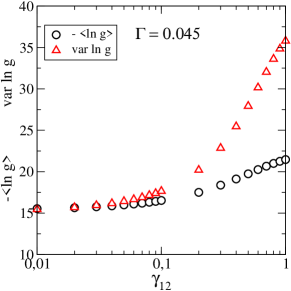
Figure 22: Mean value $\langle\ln g\rangle$ and variance var $\ln g$ as a function of $\gamma_{12}$ in the strongly insulating regime, calculated from analytical distribution (85). As expected, var $\ln g\approx-\langle\ln g\rangle$ for $\gamma_{12}\ll 1$ but var $\ln g\approx-2\langle\ln g\rangle$ for $\gamma_{12}=1$. Note that both mean and variance depends only weakly on $\gamma_{12}$ when $\gamma_{12}$ is small (which is always the case when the system size $L$ is large).

We do a saddle point analysis of Eq. (88) to obtain $\langle\ln g\rangle$ and var($\ln g$) as a function of $\Gamma$. In order to illustrate the difference between Q1D and 3D insulators, we will keep the general expressions without using the condition $\gamma_{12}\ll 1$. The free energy can be written as

$$F_{approx}=\frac{\Gamma}{4}(x-\frac{1}{\Gamma})^{2}-\ln(2x_{2min}-x);\;\;\;x=\ln(1/g).$$ (89)

The saddle point solution of the mean $x_{m}\equiv\langle\ln g\rangle$ is obtained from $F^{\prime}(x_{m})=0$ where the prime denotes derivative with respect to $x$. Denoting

$$x_{m}=1/\Gamma-y$$ (90)

this gives $y(y-\gamma_{12}/\Gamma)=2/\Gamma$, leading to

$$y=\frac{1}{2}\left[\sqrt{(\frac{\gamma_{12}}{\Gamma})^{2}+\frac{8}{\Gamma}}-\frac{\gamma_{12}}{\Gamma}\right].$$ (91)

The variance $\delta x$ can be estimated from $1/F^{\prime\prime}(x_{m})$, giving

$$\delta x\approx\frac{1}{\frac{\Gamma}{2}+\frac{\Gamma^{2}y^{2}}{4}}.$$ (92)

In the limit $\gamma_{12}\rightarrow 0$ appropriate for our 3D insulators, $y\rightarrow\sqrt{2/\Gamma}$. On the other hand in the Q1D limit $\gamma_{12}^{Q1D}=1$, $y\rightarrow 2$. Thus compared to the Q1D result $\langle\ln g\rangle^{Q1D}\approx 1/\Gamma$, the 3D result is shifted by $\sqrt{2/\Gamma}$. Similarly, compared to the Q1D result var($\ln g)=2/\Gamma$, the 3D insulators have a much sharper distribution, with half the variance $1/\Gamma$. Both results agree with numerical data. Although our model is not in general valid for $\gamma_{12}\rightarrow 1$ because of our neglect of the interaction terms, in the insulating limit the interaction terms are negligible and it is useful to see how the mean and the variance changes with $\gamma_{12}$ as it is changed from the 3D limiting value of zero to the Q1D limiting value of unity. Since $\gamma_{12}\sim\xi/2L$, for a given disorder this will correspond to starting from a cubic sample of width $L=L_{z}\gg\xi$ (where $L_{z}$ is the length) and decreasing the width to $L<\xi$ to reach the Q1D limit.

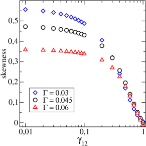
Figure 23: Skewness as a function of $\gamma_{12}$ in the strongly insulating regime. As expected, skewness is zero for $\gamma_{12}=1$ (Q1D limit).

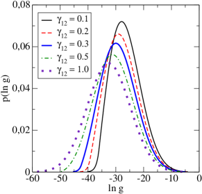
Figure 24: $P(\ln g)$ obtained from analytical formulas (Eqs. 84, 85 and 86) for $\Gamma=0.03$ and various values of $\gamma_{12}$.

Figure 22 shows how the mean and the variance changes with $\gamma_{12}$ according to Eqs. (90) and (92).

It is not possible to obtain a simple formula for the skewness $\langle(\ln g-\langle\ln g\rangle)^{3}\rangle/[\langle(\ln g-\langle\ln g\rangle)^{2}]^{3/2}$ except that in the limit $\Gamma\rightarrow 0$ it approaches a number of order unity. Direct evaluation of the quantity as a function of $\gamma_{12}$ is shown in Fig. 23, which shows that for a given disorder, the skewness starts from zero in the Q1D limit, as is well known, but saturates to a finite value (depending on disorder) in the 3D limit. It shows that the distribution is never log-normal for 3D insulators. It also shows that the distribution $P(\ln g)$ is almost independent of $\gamma_{12}$ provided that both $\gamma_{12}$ and $\Gamma$ are small. This explains why the distribution shown in Fig. 25 does not depend on the ratio $\Gamma/\gamma$.

Finally, Fig. 24 shows how the entire distribution $P(\ln g)$ changes as a function of $\gamma_{12}$, from a sharp, skewed form for $\gamma_{12}\ll 1$ to a broad Gaussian form for $\gamma_{12}=1$.

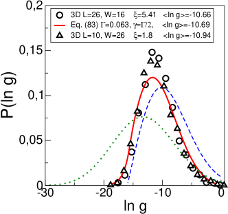
Figure 25: Conductance distribution for 3D insulators obtained from direct numerical simulation for $W=16$, $L=26$ (circles), and from Eq. (85) for $\Gamma=0.063$ and $\gamma_{12}=\Gamma/2$ (solid line). Both have the same mean value $\langle\ln g\rangle\approx-10.6$. Dashed and dotted lines show Eq. (88) with $x_{\rm 2min}=1/2\Gamma+3/4$ and $x_{\rm 2min}=1/\Gamma$, respectively, with $\Gamma=0.063$. Shown are also numerical data for $W=26$ and $L=10$ (triangles). Similar agreement is obtained for other values of $\langle\ln g\rangle$ if $\Gamma$ is used as a free parameter; see Ref. [mmwk, ] for the case $\langle\ln g\rangle\approx-12.6$ fitted with $\Gamma=0.054$ noteG/g .

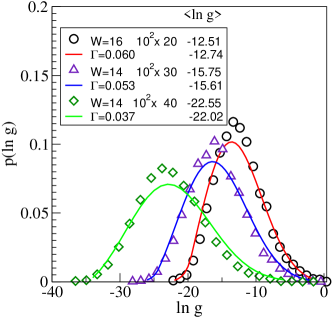
Figure 26: Conductance distribution for insulating samples of the size $L^{2}\times L_{z}$ ($L=10$) In contrast to 3D system (fig. 25), parameter $\Gamma/\gamma_{12}<1$. From numerical data, we have $\Gamma=0.3$, $\gamma_{12}=0.22$ for $W=16$, and $\Gamma=0.133~{}(0.102)$, $\gamma_{12}=0.32~{}(0.36)$ for systems with $W=14$ and $L_{z}=30$ (40), respectively. Solid lines show analytical result, Eq. (85) with $\gamma_{12}$ and $\langle\ln g\rangle$ as given form numerical data.

VII.2 Comparison with numerical data

When comparing our theoretical prediction, Eq. (85), with numerical data, we distinguish two cases: (1) for 3D systems, both $\Gamma$ and $\gamma_{12}$ decreases $\sim 1/L$, while the ratio $\Gamma/\gamma_{12}$ does not depend on $L$. (2) for systems $L^{2}\times L_{z}$, $\Gamma\sim 1/L_{z}$ while $\gamma_{12}\sim 1/L$ does not depend on $L_{z}$ (see fig. 5). Therefore, contrary to 3D geometry, $\Gamma/\gamma_{12}\ll 1$ for $L_{z}\gg L$. This different behavior of parameters $\Gamma$ and $\gamma_{12}$ explains difference between the shape of $p(\ln g)$ in 3D and Q1D strongly disordered systems, shown in figures 25 and 26.

Figure 25 shows Eq. (88) compared with the results from direct integration of Eq. (85), both compared with numerical results based on Eq. (13). For the analytic curves, we chose $\Gamma=0.063$ and $\gamma_{12}=\Gamma/2$ to have the same $\langle\ln g\rangle$ as in the numerical case noteG/g . Note that using the Q1D result $\gamma_{12}^{Q1D}=1$ gives $x_{2min}\approx 1/\Gamma$, leading to a log-normal distribution (see dotted line in Fig. (25)). As shown in [mmwk, ], variance and skewness calculated from direct integration of Eq. (85) compares well with numerical results, consistent with saddle point results from Eq. (88).

Figure 26 compares theoretical formula, Eq. (85) with numerical data for $p(\ln g)$ for insulating samples $L^{2}\times L_{z}$. While $\Gamma$ is small, decreasing as $\sim 1/L_{z}$, $\gamma_{12}$ does not depend on $L_{z}$ and is constant for fixed $L$. Consequently, ratio $\gamma_{12}/\Gamma\sim L_{z}/L$ increases with increasing $L_{z}$.

Both figures 25 and 26 show qualitative agreement with numerical data and theoretical model. Quantitative differences between Eq. (85) and numerical results have origin in our simplified model Eq. (21), which still overestimates the strength of the interaction for higher channels.

It is important to note that in both figures 25 and 26 we compared numerical data with theoretical model with the same mean $\langle\ln g\rangle$. This is consistent with scaling theory of localization since there is only one parameter - for instance $\langle\ln g\rangle$ - which determines $p(\ln g)$ completely. In order to make sure that the analytical model has the same $\langle\ln g\rangle$ as the numerical data for a given disorder, we used $\Gamma$ as a free fitting parameter. Of course we could use Eq. (20) to obtain $\Gamma$ independently for a given disorder. However, in order to do that we will need a good estimate of the mean free path $\ell$. This is difficult in the strongly disordered regime because the mean free path defined as the decay length of the single particle Green’s function is actually smaller than the lattice spacing in the strongly disordered regime economou , and our numerical model does not allow us to obtain such small lengths with good accuracy. While independent calculations of the mean free path are available for cubic systems below critical disorder economou (e.g. $\ell=0.234$ for $W=15$ in the isotropic case), there is no data available in the insulating regime. We therefor use $\Gamma$ as a free parameter. Nevertheless, as a consistency check, we estimate $\ell$ from a plot of $K_{11}L$ vs $x_{1}$ (fig. 19a), where the slope should give the mean free path (equivalently, we could identify $\Gamma^{-1}$ with numerical value of $x_{1}$). The results are plotted as the inset in fig. 27 to show the mean free path as a function of disorder. Using this result, we can estimate the value of $\Gamma$ corresponding to the disorder $W=16$ used in fig. 25. We find that $\ell(W=16)\approx 0.48$ and $\Gamma=0.070$, which is close to the fitting value $0.063$. This shows that while we can not obtain $\Gamma$ accurately enough in our present numerical scheme, the fitted values are consistent with our crude estimates. As a further consistency check, we use the above estimate of the mean free path to plot in fig. 27 the $\Gamma$ dependence of $\langle\ln g\rangle$. It shows that $\langle\ln g\rangle$ is indeed an unambiguous function of $\Gamma$, as required by the theory.

Finally, we have checked the effects of fluctuations of $k_{11}$ on $P(\ln g)$ by integrating the conductance distribution in fig. 25 over the distribution $P(k_{11})$ (fig. 4). We find that the effects are negligible.

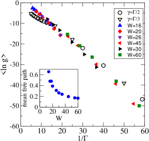
Figure 27: Mean value $\langle\ln g\rangle$ as a function of $1/\Gamma$. Open symbols: analytical result, Eq. (85). Data confirm linear dependence $\langle\ln g\rangle\propto 1/\Gamma$ for small $\Gamma$ (strong disorder). For smaller disorder (larger $\Gamma$) analytical model is less accurate. Data confirm that $\langle\ln g\rangle$ does not depend on $\gamma_{12}$ provided that both $\Gamma$ and $\gamma_{12}$ are small. Full symbols: numerical data with $\Gamma^{-1}=LK_{11}/\ell$. We estimate $\Gamma$ for a given disorder using the mean free path $\ell$ obtained from data in fig. 19a ($\ell(W)$ is shown in inset) and the relation $K_{11}L=x_{1}\ell$. Numerical $\langle\ln g\rangle$ is an unambiguous function of $\Gamma$, as required in the analytical model. Small deviations are due to finite size effects which affect actual values of parameters $x_{1}$ and $K_{11}$.

VIII Beyond the insulating limit

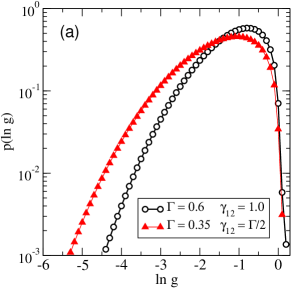
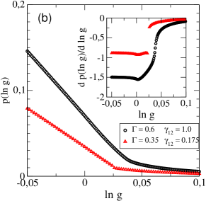
Figure 28: (a) Probability distribution $P(\ln g)$ for $\Gamma\sim 1$ where critical regime is expected. The distribution agrees qualitatively with numerical data for the critical regime. Figure (b) shows detail of the distribution shown for $\Gamma=0.35$, $\gamma_{12}=\Gamma/2$ and for $\Gamma=0.6$, $\gamma_{12}=1$. It shows that there is indeed a non-analyticity in the distribution close to $\ln g=0$ with position of the non-analyticity at $\ln g>0$, in agreement with analytical results mu-wo-ga-go-03 .

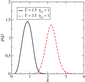
Figure 29: Analytic result for the metallic regime ($\Gamma>1$ and $\gamma_{12}=1$). Data confirm that the distribution $P(g)$ is Gaussian with variance var $g=0.064$ for $\Gamma=1.5$ and var $g=0.09$ for $\Gamma=3.5$ which is comparable to the UCF value.

From numerical simulations MK-PM ; markos1 we know that the critical regime in 3D is also dominated by only a few eigenvalues $x_{i}\gg 1$. However, since $\gamma_{12}$ is neither $0$ nor $2$, it seems that we may not be able to use the free fermion ($\eta=0$) solution of Eq. (26) to obtain the distribution of the transmission levels. However, as shown in [caselle, ], the solution is independent of the strength of the interaction $\eta$ in the strong disorder regime characterized by $x_{i}\gg 1$. This means that our solutions might be used, albeit only qualitatively, even near the critical regime. We show in Fig. (28) the distribution $P(\ln g)$ for $\Gamma\sim 1$ which is expected to be near the critical regime. It agrees qualitatively well with numerical results at the critical point, including a discontinuity in the slope near $g=1$. It is known from analysis of the Q1D systems mu-wo-ga-go-03 that separating out an additional level helps to study the non-analyticity near $g=1$. We therefore expect to obtain better results near the critical regime by separating out an additional level.

Finally, we show in Fig. 29 the distribution $P(g)$ for $\Gamma>1$ and for $\gamma_{12}=1$ which corresponds to the metallic regime. Although we do not expect that our approximate formula works quantitatively for the metallic regime, Eq. (85) gives, for this choice of the parameters, a Gaussian distribution of the conductance. Also the width of the distribution qualitatively agrees with the universal conductance fluctuations ucf in this regime. This shows that our simple model already captures the essential qualitative features at all strengths of disorder.

IX Summary and conclusion

We systematically analyzed the length and disorder dependence of the matrix $K$ to check if the generalized DMPK equation proposed in [mu-go-02, ] is valid in three dimensional systems at all strengths of disorder.

We studied the matrix $K$ in detail. The goal was to test the assumptions on which the generalized DMPK equation was derived and to construct a simple analytically tractable model for $K$ which captures all the important qualitative features. In particular, since Q1D systems have been studied in great detail, we looked for any major qualitative differences in the structure of $K$ between Q1D and 3D systems.

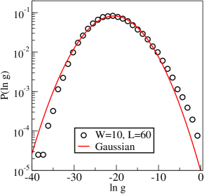
Figure 30: Typical form of the distribution $p(\ln g)$ in 2D disordered systems compared with Gaussian distribution with the same mean value and variance. $\langle\ln g\rangle=-20.6$, var $\ln g=23.5$ and skewness is 0.251. Figure indicates that the deviation from the Gaussian distribution exists in 2D as well.

We find that to a good approximation, the generalized DMPK equation remains qualitatively valid for any disorder. We also conclude that to a good approximation, we can use only two parameters, $K_{aa}\approx K_{11}$ and $\gamma_{ab}\approx\gamma_{12}$, to characterize the qualitative changes in transport at different strengths of disorder in different dimensions. We find that although fluctuations in $k_{11}$ at strong disorder are large (non self-averaging), the effect of these fluctuations on $P(\ln g)$ is negligible. More importantly, we do not have an independent way to estimate the mean free path to obtain $\Gamma=\ell/(L_{z}K_{11})$, but all qualitative features of the entire distribution $P(\ln g)$ is obtained correctly once an effective $\Gamma$ is used as a free parameter. We also find how these parameters depend on disorder and show their unambiguous dependence on the localization length. This is important since it indicates that the introduction of new parameters does not necessarily invalidate the single parameter scaling theory of localization.

We have also shown that the matrix $K$ contains information about the Anderson transition. The scaling of the parameters $LK_{11}$ or $\gamma_{12}$ clearly identifies the critical point which agrees with numerical results.

We then concentrate on the strong disorder limit where our numerical results allowed us to construct a simple one-parameter model of the matrix $K$, containing $\Gamma=\ell/K_{11}L_{z}$ and $\gamma_{12}=2K_{12}/K_{11}$, with $\Gamma/\gamma_{12}=2$. By varying $\gamma_{12}$, we show how one can go from a Q1D ($\xi\gg L$) to a truly 3D ($\xi\ll L$) system in the insulating regime, which clearly shows the difference between a Q1D and a 3D insulator. We then use the model to obtain the full distribution $P(g)$ which agrees qualitatively with numerical results.

It is indeed remarkable that even though the generalized DMPK equation (24) neglects fluctuations in $k_{ab}$ and the model Eq. (19) neglects the index dependence of $K_{ab}$, the theory still captures all the essential features of length, disorder as well as dimensionality dependence of the entire conductance distribution and provides in particular a simple understanding of the 3D distribution at strong disorder, which is qualitatively different from a log-normal distribution in Q1D. At the same time, our numerical studies suggest that having an independent estimate of the mean free path could provide a more quantitative description of the conductance distribution in 3D at all disorder.

We emphasize that there are large differences between Q1D and higher dimensions. In Q1D defined in [mu-wo-99, ; go-mu-wo-02, ; mu-wo-ga-go-03, ; dmpk, ], disorder is always weak enough to assure that the localization length $\xi\gg L$ where $L$ is the transverse dimension. The Q1D insulator corresponds to the weakly disordered systems of length $L_{z}\gg\xi$. It is this length-induced insulating behavior that is described by the DMPK equation. This is different from localization in 3D which occurs at strong disorder, where $\xi$ is much less than both $L_{z}$ and $L$. This difference is clearly reflected in the matrix $K$, where Table I summarizes how the scale dependence of $K_{11}$ and $\gamma_{12}$ depend on disorder in 3D. In contrast, $K$ in Q1D is independent of disorder. Our model recovers all the peculiarities of the 3D localized regime: we found that the distribution $P(\ln g)$ is narrower than in Q1D and possesses non-zero skewness.

Although we concentrated on 3D systems, general considerations about the properties of the matrix $K$ in the insulating regime should be valid in any dimension $d>2$. In particular, the assumption that $K_{11}$ is a nonzero $L$-independent constant in the localized regime is correct independent of dimensionality. Therefore, we expect that our theory of the insulating regime is valid for any $d>2$. Consequently, the distribution $P(\ln g)$ is not Gaussian in the localized regime in any $d>2$, although the nature of the deviation from the Gaussian form might be dimensionality dependent. In fact we expect $P(\ln g)$ to be different from Gaussian distribution even in 2D markos2 . This expectation is supported by Fig. 30 which shows $P(\ln g)$ for a 2D square system obtained numerically using Eq. 13. As discussed in the paper, deviations from the Gaussian form are due to the changes of the spectrum of parameters $x$. Although the contribution of the first channel to the conductance is dominant, higher channels do influence the statistical properties of the smallest parameter, $x_{1}$. This effect was probably not considered in previous analytical works which predict Gaussian distributions of $\ln g$ in the insulating regimes in dimensions $d=2+\epsilon$ altshuler .

When applied to the critical regime, our theory recovers typical properties of the conductance distribution, including the non-analyticity of the distribution in the vicinity of $g=1$. Although our present results are only qualitatively correct in the critical regime, we believe that the method developed in the paper represents a good starting point for further development of the theory of Anderson transition.

KAM thanks U. Karlsruhe for support and hospitality during his visit. PM thanks APVT, grant n. 51-021602 for financial support. PW gratefully acknowledges support of a visit and hospitality at the U. Florida as well as partial support by a Max-Planck Research Award.

References

- (1) K. A. Muttalib, P. Wölfle and V. A. Gopar, Ann. Phys. 308, 156 (2003).
- (2) J.-L. Pichard, in B. Kramer (ed.) Quantum Coherence in Mesoscopic Systems NATO ASI 254, Plenum Press NY and London (1991).
- (3) A. García-Martin and J. J. Sáenz, Phys. Rev. Lett. 87, 116603 (2001); A. García-Martin, M. Governale and P. Wölfle, Phys. Rev. B 66, 233307 (2002);
- (4) K. A. Muttalib and P. Wölfle, Phys. Rev. Lett. 83,3013 (1999); P. Wölfle and K.A. Muttalib, Ann. Phys. (Leipzig) 8, 753 (1999).
- (5) V. A. Gopar, K. A. Muttalib and P. Wölfle, Phys. Rev B 66, 174204 (2002); L. S. Froufe-Perez, P. García-Mochales, P. A. Serena, P. A.Mello and J. J. Sáenz, Phys. Rev. Lett. 89, 246403 (2002) .
- (6) K. A. Muttalib, P. Wölfle, A. Garcia-Martin and V. A. Gopar, Europhys. Lett. 61, 95 (2003); A. García-Martin and J. J. Sáenz, Phys. Rev. Lett. 87, 116603 (2001).
- (7) P. Markoš and B. Kramer, Philos. Mag. B 68, 357 (1993);
- (8) P. Markoš, Phys. Rev. Lett. 83, 588 (1999); M. Rühländer, P. Markoš and C.M. Soukoulis, Phys. Rev. B 64, 212202 (2001).
- (9) B. K. Nikolic, P. B. Allen, Phys. Rev. B 63, 020201 (2001); M. Rühländer, P. Markoš and C.M. Soukoulis, Phys. Rev. B 64, 172202 (2001);
- (10) K. Slevin, P. Markoš and T. Ohtsuki, Phys. Rev. Lett. 86, 3594, (2001)
- (11) P. Markoš, Phys. Rev. B 65, 104207 (2002); P. Markoš in Anderson Transition and its Ramifications, eds. T. Brandes and S. Ketteman, Lecture Notes in Physics vol. 630, Springer 2003.
- (12) B.L. Altshuler, V.E. Kravtsov and I. Lerner, Sov. Phys. JETP 64, 1352 (1986), and Phys. Lett. A 134, 488 (1989).
- (13) B. Shapiro, Phys. Rev. Lett. 65, 1510 (1990); A. Cohen and B. Shapiro, Int. J. Mod. Phys. B 6, 1243 (1991).
- (14) K. A. Muttalib and V. A. Gopar, Phys. Rev B 66, 115318 (2002); K. A. Muttalib and J. R. Klauder, Phys. Rev. Lett. 82, 4272 (1999).
- (15) P. Markoš, K. A. Muttalib, P. Wölfle and J. R. Klauder, Europhys. Lett. 68, 867 (2004)
- (16) E. Abrahams, P. W. Anderson, D. C. Licciardello, T. V. Ramakrishnan, Phys. Rev. Lett. 42, 673 (1979); A. MacKinnon, B. Kramer, Phys. Rev. Lett. 47, 1546 (1981).
- (17) See e.g. A. D. Stone, P. Mello, K. A. Muttalib and J-L. Pichard in Mesoscopic phenomena in solids, eds. B. L. Altshuler, P. A. Lee and R. A. Webb, North-Holland, 369 (1991).
- (18) O. N. Dorokhov, JETP Lett. 36, 318 (1982); P. A. Mello, P. Pereyra and N. Kumar, Ann. Phys. (N.Y. ) 181, 290 (1988).
- (19) R. Landauer, IBM J. Res. Dev. 1, 223 (1957).
- (20) For a recent review, see Ya.M. Blanter and M. Büttiker, Phys. Rep. 336, 1 (2000).
- (21) C.W.J. Beenakker, Phys. Rev. B 46, R12841 (1992).
- (22) , see J.-L. Pichard in [pichard-nato, ].
- (23) I. Zambetaki, Q. Li, E. N. Economou and C. M. Soukoulis, Phys. Rev. Lett. 76, 3614 (1996).
- (24) J. B. Pendry, A. MacKinnon, and P. J. Roberts, Proc. R. Soc. London A 437, 67 (1992). T. Ando, Phys. Rev. B 44, 8017 (1989)
- (25) J.-L. Pichard, N. Zannon, Y. Imry, J. Phys. France 51, 587 (1990).
- (26) J.T. Chalker and M. Bernhardt, Phys. Rev. Lett. 70, 982 (1993).
- (27) Note that for , must decrease as . Indeed, from (9) we have so that the sum of positive parameters is in the insulating regime. We ignore this detail in our model.
- (28) P. Markoš J. Phys.: Condens. Matt. 7, 8361 (1995).
- (29) In Ref. [mmwk, ] we used . This difference is not important, since, as we show in Fig. 23, the actual value of does not influence the value of the skewness when both and are small.
- (30) C. W. J. Beenakker and B. Rejaei, Phys. Rev. Lett. 71, 3689 (1993); Phys. Rev. B 49, 7499 (1994).
- (31) E. N. Economou, C. M. Soukoulis and A. D. Zdetsis, Phys. Rev. B 31, 6483 (1985).
- (32) M. Caselle, Phys. Rev. Lett. 74, 2776 (1995).
- (33) B.L. Altshuler, JETP Lett. 41, 648 (1985); P.A. Lee and A.D. Stone, Phys. Rev. Lett. 55, 1622 (1985).