Field-angle resolved specific heat and thermal conductivity in the vortex phase of UPd₂Al₃

Abstract

The field-angle dependent specific heat and thermal conductivity in the vortex phase of UPd₂Al₃ is studied using the Doppler shift approximation for the low energy quasiparticle excitations. We first give a concise presentation of the calculation procedure of magnetothermal properties with vortex and FS averages performed numerically. The comparison of calculated field-angle oscillations and the experimental results obtained previously leads to a strong reduction of the possible SC candidate states in UPd₂Al₃. The possible SC gap functions have node lines in hexagonal symmetry planes containing either the zone center or the AF zone boundary along c. Node lines in non-symmetry planes can be excluded. We also calculate the field and temperature dependence of field-angular oscillation amplitudes. We show that the observed nonmonotonic field dependence and sign reversal of the oscillation amplitude is due to small deviations from unitary scattering.

I Introduction

The U-based heavy fermion (HF) superconductors (SC) are supposed to have unconventional SC order parameters usually (but not necessarily) associated with anisotropic gap functions $\Delta$(k) that have node points or lines on the Fermi surface (FS) where $\Delta$(k) = 0 Sigrist and Ueda (1991); Thalmeier and Zwicknagl (2004). This is thought to be the result of a purely electronic mechanism of Cooper pair formation which favors anisotropic gap functions due to a strong on-site heavy quasiparticle repulsion. The type and position of nodes in $\Delta$(k) is intimately connected with the symmetry class to which $\Delta$(k) belongs, in most cases described by a single irreducible representation of the high temperature symmetry group Volovik and Gor’kov (1985); Mineev and Samokhin (1999). Experimental evidence for the presence of node lines is obtained from thermodynamic and transport quantities as well as resonance experiments, but to locate their exact position on the FS and hence restrict the number of possible representations for the SC order parameter is a difficult task. For example in UPt₃ it took a considerable time until it was identified as the two-dimensional odd parity (spin-triplet) E_2u representation and still there is no unanimous agreement on this symmetry Joynt and Taillefer (2002).

Recently the experimental determination of SC gap symmetries has been much facilitated by the advent of a new method, namely the investigation of field-angle dependence of specific heat and thermal conductivity at temperatures T $\ll$ T_c. From the typical angular oscillations observed in these quantities under favorvable conditions (small quasiparticle scattering) one may deduce the position of the nodal lines or points of $\Delta$(k) with respect to the crystal axis. Knowledge of these positions narrows down the possible choices of representations for $\Delta$(k) considerably. This method has been sucessfully applied to unconventional organic SC Izawa et al. (2002a), to ruthenates Izawa et al. (2001a), borocarbides Izawa et al. (2002b); Park et al. (2003) and Ce,Pr-based HF superconductors Izawa et al. (2001b, 2003); Aoki et al. (2004). It is based on the ’Volovik effect’ Volovik (1993) which means the appearance of quasiparticle states in the inter-vortex region of unconventional SC due to the presence of nodes with $\Delta$(k) = 0 along certain directions in k-space. The zero energy density of states (ZEDOS) of these continuum states and hence their contribution to specific heat and thermal conductivity depends on the relative orientation of field direction, nodal positions and crystal axes through the superfluid Doppler shift (DS) effect of quasiparticle energies. This results in the angular oscillations of specific heat and thermal conductivity which contain important information on the nodes of the gap function.

In addition this method has now been applied for the first time to a U-based superconductor Watanabe et al. (2004), namely the intermetallic moderate HF ($\gamma$ = 140 $\frac{mJ}{molK^{2}}$) compound UPd₂Al₃ Geibel et al. (1991). This compound was in the focus of interest in recent years because it is the only HF superconductor where direct evidence for the microscopic nature of the SC pairing mechanism has been found. This is connected with the fact that UPd₂Al₃ is the most clear cut example of a U-based superconductor (SC) with dual-nature 5f electrons, some of which are localised and some itinerant. The former can be considered as 5f² CEF states and the latter as conduction band states Zwicknagl et al. (2003). The mass enhancement of conduction electrons (m^∗/m${}_{b}\sim$ 10, m_b is the band mass) is a result of their interaction with the propagating CEF-excitations (‘magnetic excitons’) associated with the localised 5f electrons. The induced-moment AF order with T_N = 14.3 K, Q = (0,0,0.5) (r.l.u.) and moderately large $\mu$ = 0.85$\mu_{B}$ coexists with SC below T_c = 1.8 K. In complementary INS Bernhoeft (2000); Sato et al. (2001) and quasiparticle tunneling experiments Jourdan et al. (1999) both 5f components were investigated and it was concluded Sato et al. (2001) that magnetic excitons mediate Cooper pairing. Theoretically this new pairing mechanism was investigated in Thalmeier (2002); McHale et al. (2004) and possible symmetries of the SC states were discussed, also in connection with existing Knight shift Kitaoka et al. (2000) and upper critical field results Hessert et al. (1997). The conventional itinerant spin fluctuation mechanism has been investigated in Nishikawa and Yamada (2002); Oppeneer and Varelogiannis (2003) and also in Thalmeier (2002).

The plausible SC gap functions obtained in McHale et al. (2004) from a microscopic model predict a node line parallel to the hexagonal ab-plane but several D_6h representations with different parity are possible solutions. Furthermore the alternative spin fluctuation model of Nishikawa and Yamada (2002) predicts node lines perpendicular to the basal plane. Therefore further investigation of the gap structure of UPd₂Al₃ has turned out to be necessary. It was already suggested in Thalmeier and Maki (2002) that field-angle resolved experiments might be helpful to clarify the situation. They have now indeed been performed in Watanabe et al. (2004).

The purpose of this paper is twofold: Firstly, although the theory of magnetothermal properties in superconductors on the basis of the DS approximation is well developed, the results are scattered through the literature and therefore we first give a concise and complete outline of the necessary computational steps for SC with uniaxial symmetry in the superclean limit. The calculation of linear specific heat coefficient $\gamma$(T,H) = C(T,H)/T and thermal conductivity $\kappa_{ii}$(T,H) (i = x,z,y) involves averaging over both quasiparticle momenta and energies and the vortex coordinate. For quantitative predictions the five-fold integrations are carried out fully numerically for each of the candidate gap functions. Also this has the advantage that one can study the temperature dependence of oscillation amplitudes and real FS geometry effects. Secondly we want to apply the DS theory in detail to UPd₂Al₃ and study the predicted field-angle variations of the above quantities for the possible gap functions with special emphasis on the problem of node-line position along c^∗. We also discuss the influence of FS cylinder corrugation on field angle dependence and the temperature variation of angular oscillation amplitudes and investigate the dependence on the scattering phase shift.

In Sect. II we introduce the concept of the Doppler shift approximation for quasiparticle energies and in Sect. III we give the explicit expression for this quantity in two FS geometries. In Sect. IV we define the necessary averages over vortex coordinates (superfluid velocity field) in the single-vortex approximation. The calculation procedure for specific heat and thermal conductivity in the superclean limit is given in Sect. V. Then in Sect. VI we apply the theory to UPd₂Al₃ and discuss the results for the most prominent candidate gap function in view of the available experimental results in Watanabe et al. (2004). Finally Sect. VII presents our conclusion on the gap symmetry of UPd₂Al₃ and an outlook on theoretical developments.

II Doppler shift of SC quasiparticles in the vortex phase

In the vortex state the superfluid has acquired a velocity generated by the gradient of the condensed phase as given by

$${\bf v}_{s}=\hbar\tensor{m}^{-1}(\nabla\phi-\frac{2e}{\hbar c}{\bf A})=\hbar\tensor{m}^{-1}\tilde{\nabla}\phi$$ (1)

It is connected to the screening current circulating the vortex by

$${\bf j}_{s}({\bf r})=2en_{s}({\bf r}){\bf v}_{s}({\bf r})=\frac{c}{4\pi}\nabla\times{\bf h}({\bf r})$$ (2)

Here $m_{ij}=m_{a}\delta_{ij}+(m_{c}-m_{a})\hat{n}_{i}\hat{n}_{j}$ is the uniaxial mass tensor with $\hat{{\bf n}}$ giving the symmetry axis. Furthermore n_s(r) is the superfluid density and h(r) is the local magnetic field strength. The above equations hold for large Ginzburg parameters when local London electrodynamics is applicable Balatskii et al. (1986); Bulaevskii (1990).

Quasiparticle excitations out of the condensate with momentum p_L have an energy E_L(p_L) in the local rest frame of the superfluid. The transformation to the laboratory frame is given by the universal law Volovik (2004)

$${\bf p} = {\bf p}_{L}$$

$$E({\bf p},{\bf r}) = E_{L}({\bf p})+{\bf p}\cdot{\bf v}_{s}({\bf r})$$ (3)

The second equation may be interpreted as a Doppler shift (DS) of quasiparticle energies due to the moving condensate. In an unconventional superconductor with gap nodes $\Delta$(k) = 0 on the FS low energy (E $\ll\Delta$) quasiparticles can tunnel to the intervortex region where they acquire a DS according to Eq. (II). Since in a nodal SC the zero-field DOS starts like a power law N(E) $\sim$ Eⁿ the DS, after averging over position r and momentum p, will lead to a non-vanishing ZEDOS N(E=0,H) of quasiparticles Volovik (1993) which determine the low temperature (T $\ll$ T_c) specific heat and thermal transport.

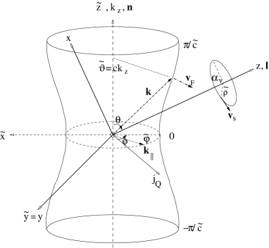
Figure 1: Geometrical configuration of corrugated FS cylinder in the AF BZ ($-\frac{\pi}{\tilde{c}}\leq k_{z}\leq\frac{\pi}{\tilde{c}}$ with $\tilde{c}=2c$), vortex direction (l) and quasiparticle momentum k. Here $\tilde{x},\tilde{y}\equiv y,\tilde{z}$ is the cartesian crystal coordinate system with a,b and c (n)-axes. The cartesian coordinate system x,y,z is rotated by the angle $\theta$ around y axis such that z ligns up with the vortex direction l. Here $\phi$ is the angle between heat current j_Q and the field rotation ($\tilde{x}\tilde{z}$-) plane. Experimentally the perpendicular configuration $\phi=90^{\circ}$ is used. Note that for uniaxial crystals the vortex polar angle $\theta$ differs from the field polar angle $\theta_{H}$, this misallignment is given by Eq. (33) and shown in the inset of Fig. 2. The quasiparticle momentum k is described by cylindrical coordinates ($\tilde{\vartheta}=ck_{z},\tilde{\varphi}$) and v_F $\perp$ FS denotes the quasiparticle velocity. The superfluid velocity is denoted by ${\bf v}_{s}$ and $\alpha_{v}$, $\tilde{\rho}$ are the vortex coordinates.

III superfluid velocity in the London limit

The superfluid velocity field v_s(r) is obtained from the field distribution h(r) according to Eq. (2). In the London limit ($\lambda_{i}\gg\xi_{i}$; i=a,c with $\parallel\equiv$a, $\perp\equiv$c) the latter is determined by the equation

$${\bf h}+\lambda_{\parallel}^{2}\nabla\times(\nabla\times{\bf h})+(\lambda_{\perp}^{2}-\lambda_{\parallel}^{2})\nabla\times[{\bf n}({\bf n}\cdot\nabla\times{\bf h})]=\hat{{\bf z}}\Phi_{0}\delta({\bm{\rho}})$$ (4)

where ${\bm{\rho}}$=(x,y) are the cartesian coordinates of the plane perpendicular to the vortex direction $\hat{{\bf l}}$ $\parallel$ $\hat{{\bf z}}$  (Fig. 1) and $\Phi_{0}=hc/2e$ is the flux quantum. In general h has components both parallel and perpendicular to $\hat{{\bf l}}$ Balatskii et al. (1986). Here we neglect the latter and in the following assume h = h(x,y)$\hat{{\bf l}}$. The superfluid velocity and field distribution in the xy-plane are not circular around the vortex in the case of a uniaxial symmetry. However, we may apply a scale transformation ${\bm{\rho}}\rightarrow{\bm{\rho}}^{\prime}$ or $(x,y)\rightarrow$(x’,y’) given by

$$x^{\prime} = \frac{x}{\lambda_{\parallel}}=\rho^{\prime}\cos\alpha_{v}$$ (5)

$$y^{\prime} = \frac{y}{\lambda_{\theta}}=\rho^{\prime}\sin\alpha_{v}$$ (6)

with $\rho^{\prime}$=[x’²+y’²]${}^{\frac{1}{2}}$ denoting the distance from the vortex center, $\alpha_{v}$ the azimuthal angle around the vortex and $\theta=\angle$($\hat{{\bf l}}$,$\hat{{\bf n}}$), see Fig. 1. This leads to a transformed h(x’,y’) determined by

$$h(x^{\prime},y^{\prime})-(\partial_{x^{\prime}}^{2}+\partial_{y^{\prime}}^{2})h(x^{\prime},y^{\prime})=\frac{\Phi_{0}}{\lambda_{\parallel}\lambda_{\theta}}\delta(x^{\prime},y^{\prime})$$ (7)

Therefore in the scaled x’,y’ coordinate system one has again a circular vortex and field distribution. The solution of Eq. (7) is given by (K₀ = Hankel function)

$${\bf h}({\bm{\rho}}^{\prime})=\frac{\Phi_{0}}{2\pi\lambda_{\parallel}\lambda_{\theta}}K_{0}(\rho^{\prime})\simeq\frac{\Phi_{0}}{2\pi\lambda_{\parallel}\lambda_{\theta}}[\ln\frac{1}{\rho^{\prime}}+0.12]$$ (8)

The scaled superfluid velocity field v’_x=v_x/$\lambda_{\parallel}$, v’_y=v_y/$\lambda_{\theta}$ for distances $\rho^{\prime}\gg\xi/\lambda$ is then obtained from Eq. (2) as

$${\bf v}^{\prime}_{s}({\bm{\rho}}^{\prime})=\frac{\hbar}{4m\lambda^{2}}\frac{1}{\rho^{\prime}}\left(\matrix{-\sin\alpha_{v}\cr\cos\alpha_{v}\cr 0}\right)$$ (9)

where $\lambda=(\lambda_{\parallel}\lambda_{\theta})^{\frac{1}{2}}$, $\xi=(\xi_{\parallel}\xi_{\theta})^{\frac{1}{2}}$ and $m=(m_{\parallel}m_{\theta})^{\frac{1}{2}}$ are defined in App. B. The scaled $\rho^{\prime}$ coordinate is dimensionless. We may reintroduce length dimension but keep the circular vortex shape by defining

$$\tilde{\rho}=\lambda\rho^{\prime}\quad,\quad\tilde{{\bf v}}_{s}=\lambda{\bf v}_{s}^{\prime}\quad,\quad$$ (10)

In the rotated coordinate system (x,y,z) of Fig. 1 with the z-axis alligned with the vortex direction $\hat{{\bf l}}$, the scaled quasiparticle velocities defined in App. A are transformed to

$${\bf v}_{F}^{\prime}=\left(\matrix{\lambda_{\parallel}^{-1}[v_{a}(\tilde{\vartheta})\cos\theta\cos\tilde{\varphi}+v_{c}(\tilde{\vartheta})\sin\theta]\cr\lambda_{\theta}^{-1}[v_{a}(\tilde{\vartheta})\sin\phi]\cr\quad[-v_{a}(\tilde{\vartheta})\sin\theta\cos\tilde{\varphi}+v_{c}(\tilde{\vartheta})\cos\theta]}\right)$$ (11)

Here $v_{i}(\tilde{\vartheta})=v_{i}^{0}\hat{v}_{i}(\tilde{\vartheta})$ where $\tilde{\vartheta}$ is the polar angle for an ellipsoidal FS and $\tilde{\vartheta}=ck_{z}$ for the cylindrical FS of App. A. Furthermore ($\tilde{\varphi}$,$\tilde{\vartheta}$) defines the direction of quasiparticle momentum on the FS and $\theta$ is the vortex tilt angle in the field rotation plane which for convenience is chosen as the $\tilde{x}\tilde{z}$-plane.

The dimensionless Doppler shift energy x (not to be confused with the cartesian coordinate) for a given vortex direction is then given by

$$x=\frac{{\bf p}_{F}\cdot\tilde{{\bf v}}_{s}}{\Delta}=\frac{1}{\Delta}m\tilde{{\bf v}}_{F}(\tilde{\vartheta},\tilde{\varphi};\theta)\cdot\tilde{{\bf v}}_{s}(\tilde{\rho},\alpha_{v})$$ (12)

with $\tilde{{\bf v}}_{F}=\lambda{\bf v}_{F}^{\prime}$ and $\tilde{{\bf v}}_{s}$ defined by Eqs. (9),(10) and $\Delta$ denoting the SC gap amplitude. Using Eqs. (9),(11) we finally obtain for x = x($\theta,\tilde{\vartheta},\tilde{\varphi};\tilde{\rho},\alpha_{v}$) the explicit result

$$x=\frac{1}{4}\frac{\xi_{a}^{0}}{\tilde{\rho}}\Bigl{\{}\bigl{(}\frac{\lambda_{\parallel}}{\lambda}\bigr{)}\hat{v}_{a}(\tilde{\vartheta})\sin\tilde{\varphi}\cos\alpha_{v}-\bigl{(}\frac{\lambda_{\theta}}{\lambda}\bigr{)}[\hat{v}_{a}(\tilde{\vartheta})\cos\theta\cos\tilde{\varphi}+\alpha^{\frac{1}{2}}\hat{v}_{c}(\tilde{\vartheta})\sin\theta]\sin\alpha_{v}\Bigr{\}}$$ (13)

where $\sqrt{\alpha}=v_{c}^{0}/v_{a}^{0}$ is the anisotropy of the Fermi velocity, $\xi_{a}^{0}=(\hbar v_{a}^{0}/\pi\Delta)$ is the in-plane coherence length and $\hat{v}_{a,c}(\tilde{\vartheta})$ are given in App. A. Thus the Doppler shift energy of a quasiparticle depends on three sets of variables: The vortex direction ($\theta$) (or field direction $\theta_{H}$), see App. B), the quasiparticle momentum coordinates ($\tilde{\vartheta},\tilde{\varphi}$) on the FS and the quasiparticle position in real space ($\tilde{\rho},\alpha_{v}$) with respect to the vortex center. The expression in Eq.(13) is the central quantity which determines the thermodynamic and transport properties in the vortex phase. In the special case for H $\parallel$ c ($\theta=0$) the DS simplifies to

$$x=\frac{1}{4}\frac{\xi_{a}^{0}}{\tilde{\rho}}\hat{v}_{a}(\tilde{\vartheta})\sin(\tilde{\varphi}-\alpha_{v})$$ (14)

Because x now depends only on the angle difference $\tilde{\varphi}-\alpha_{v}$, averaging over the DS for H $\parallel$ c involves one integration less than for general field direction.

IV Average over the vortex coordinates

The calculation of thermodynamic and transport coefficients and the quasiparticle DOS involves averaging over both vortex coordinates (real space) and quasiparticle velocities (momentum space). It is instructive to calculate the vortex averaged DS energy $\langle|x|\rangle^{{\bf k}}_{v}$ of quasiparticles with given k, i.e. ($\tilde{\vartheta},\tilde{\varphi}$), as function field direction $\theta$. Since the important contributions to $\gamma$(T,H) and $\kappa_{ii}$(T,H) come from the nodal regions with $|\Delta({\bf k})|/\Delta\leq|x|$, the field-angle dependence of $\langle|x|\rangle^{{\bf k}}_{v}$ for k $\in$ nodal region gives already qualitative information on the behaviour of $\gamma$ and $\kappa_{ii}$ as shown in this section.

In the scaled coordinates x’,y’ spanning the plane perpendicular to the vortex direction $\hat{{\bf l}}$($\theta$) the field distribution h(x’,y’) and velocity distribution v_s(x’,y’) are circularly symmetric for a single vortex. In the limit H $\ll$ H_c2 the average over the vortex lattice is then approximately replaced by the integration over a single rotationally symmetric vortex according to

$$\langle A(\tilde{\rho},\alpha_{v})\rangle_{v}=\frac{1}{\pi(\tilde{d}^{2}-\tilde{d}_{c}^{2})}\int_{0}^{2\pi}d\alpha_{v}\int_{\tilde{d}_{c}}^{\tilde{d}}d\tilde{\rho}\tilde{\rho}A(\tilde{\rho},\alpha_{v})$$ (15)

Here $\tilde{d}_{c}$ is a lower cutoff of the size of the coherence length $\xi=(\xi_{\parallel}\xi_{\theta})^{\frac{1}{2}}$ and $\tilde{d}$ is of the order of the inter-vortex distance. It is determined by assuming a square vortex lattice and replacing its (square) unit cell of area F_□ by a circle of equal area with radius $\tilde{d}$ requiring $\pi\tilde{d}^{2}$ = F_□=$\Phi_{0}$/H. This leads to

$$\tilde{d}=\tilde{d}_{0}\bigl{(}\frac{H}{H_{0}}\bigr{)}^{-\frac{1}{2}}\quad;\quad\tilde{d}_{0}=\bigl{(}\frac{\Phi_{0}}{\pi}\bigr{)}^{\frac{1}{2}}\frac{1}{\sqrt{H_{0}}}=\bigl{(}\frac{hc}{2\pi}\bigr{)}^{\frac{1}{2}}\frac{1}{\sqrt{eH_{0}}}$$ (16)

Figure 2: Vortex-averaged dimensionless Doppler shift (H = 1T) as function of vortex direction $\theta$ for various quasiparticle momenta k which are given in cylindrical coordinates as ($\tilde{\vartheta}=ck_{z},\tilde{\varphi}$). Full line: ($\frac{\pi}{2}$,0); dashed line: ($\frac{\pi}{2}$,$\frac{\pi}{2}$); these k-vectors lie in the k_z=$\pi/2c$ symmetry plane which is also the nodal AF zone-boundary plane for A_1g. dash-dotted line: ($\frac{\pi}{4}$,$\frac{\pi}{2}$); this k-vector lies in a non-symmetry plane which is the nodal plane for the last gap function in Table 1. The small splitting at $\theta=90^{\circ}$ is caused by the FS corrugation. The inset shows the misallignment between vortex ($\theta$) and field ($\theta_{H}$) directions for a mass anisotropy $\alpha$=0.69 appropriate for UPd₂Al₃. In all following angular plots we use $\theta$ as variable and neglect the difference between $\theta$ and $\theta_{H}$.

with $\Phi_{0}$=(hc/2e) = 2.07$\cdot$10^-11Tcm² and H₀ = 1T the magnetic length scale involved is $\tilde{d_{0}}$(1T) = 257 Å. This means $\tilde{d}_{0}/\xi_{a}^{0}=3$ when we approximate the BCS or Pippard coherence length $\xi_{a}^{0}$ by the a,c- averaged value $\xi_{0}\sim$ 85Å given in Ref. Geibel et al. (1991) for UPd₂Al₃. This estimate has some uncertainty depending on the inclusion of Pauli limiting effects. The ratio $\tilde{d}_{0}/\xi_{a}^{0}$ determines directly the size of the DS via the prefactor in Eq. (14) when $\tilde{\rho}$ is expressed in units of $\tilde{d}_{0}$. Decreasing the ratio $\tilde{d}_{0}/\xi_{a}^{0}$ at fixed H($\tilde{d}_{0}$) increases the DS and hence the oscillation amplitudes. It is useful to check the consistency of this value in an independent way. Using the expression for H_c2 in Eq. (34) we may also write the magnetic length scale as

$$\tilde{d}_{0}=\sqrt{2}\xi_{a}^{0}\Bigl{(}\frac{H_{c2}}{H_{0}}\Bigr{)}^{\frac{1}{2}}$$ (17)

With the experimental H${}^{a}_{c2}$ = 3.2T Watanabe et al. (2004) we obtain $\tilde{d_{0}}$(1T) = 215 Å which is consistent with the previous value. The discrepancy may be due to Pauli limiting effects which reduce H_c2 Hessert et al. (1997) from its purely orbital value. These estimates also give an insight in the validity range of the single vortex and DS approximation. For fields H $\ll$ H_c2 (but large enough to fulfill $|x|\Delta\gg\ \Gamma$) we have $\xi_{0}\sim\tilde{d}_{c}\ll\tilde{d}$, consequently we may approximate $\tilde{d}_{c}\simeq 0$ in this limit. This means we commit a small error by extending the DS approximation to the core region where it is not valid.

We now perform the average in Eq. (15) for $A(\tilde{\rho},\alpha_{v})=|x(\theta;\tilde{\vartheta},\tilde{\varphi};\tilde{\rho},\alpha_{v})|$, i.e. the absolute value for the DS energy in Eq. (13) for fixed momentum k ($\tilde{\vartheta},\tilde{\varphi}$) direction. In Fig. 2 we compare $\langle|x|\rangle^{{\bf k}}_{v}$ for various quasiparticle momenta k. Keeping in mind that according to Eq. (12) $|x|$ vanishes when $\tilde{{\bf v}}_{F}\perp\tilde{{\bf v}}_{s}$ and becomes maximal for $\tilde{{\bf v}}_{F}\parallel\tilde{{\bf v}}_{s}$, the $\theta$ (or $\theta_{H}$) variation of $\langle|x|\rangle^{{\bf k}}_{v}$ in Fig. 2 can be qualitatively understood. It is the $\theta$ variation of $\langle|x|\rangle^{{\bf k}}_{v}$ for k $\in$ nodal region which survives in the ZEDOS and transport coefficients from which conclusions on the positions of nodes of $\Delta$(k) may be drawn.

V Thermodynamics and transport in the vortex phase in DS approximation

The low temperature transport and thermodynamics in unconventional SC are determined by the combined effect of impurity scattering and DS due to the supercurrents. Both effects may lead to a low energy residual DOS which influences specific heat and thermal conductivity. In the zero-field limit the theory is well developed Mineev and Samokhin (1999). Our intention here is to study typical signatures of the nodes of $\Delta$(k) in magnetothermal properties to draw conclusions on the gap structure. For this purpose the ’superclean limit’ where the DS energy dominates the effect of scattering ($|x|\Delta\gg\Gamma$) is the relevant one.

Transport and thermodynamics of unconventinal SC in DS approximation has been developed by many authors over the years, following the pioneering work of Volovik Volovik (1993), we mention only a few of them here Barash et al. (1997); Kübert and Hirschfeld (1998); Vekhter et al. (2001); Won and Maki (2000); Dahm et al. (2000); Won and Maki (2001a, b). For our purpose it is sufficient to have a summary of these results in the superclean limit in a concise form useful for numerical computation of the field-angle dependence of $\kappa_{ii}({\bf H},T)$ and $\gamma({\bf H},T)$.

Figure 3: Quasiparticle DOS for the A_1g gap function for H = 0 (full line) and 1T (dash-dotted line) and field $\parallel$ c ($\theta_{H}=\theta=0$). The DOS singularity is smeared out by the k-dependent DS. Inset shows the ZEDOS induced by the Doppler shift on an enlarged scale.

In the zero-field case the quasiparticle energies of an unconventional superconductor are given by E_k = [$\epsilon_{{\bf k}}^{2}$+ $\Delta_{{\bf k}}^{2}$]${}^{\frac{1}{2}}$ where $\Delta_{{\bf k}}$ is the nontrivial singlet gap function or $\Delta_{{\bf k}}^{2}=|{\bf d}_{{\bf k}}|^{2}$ with ${\bf d}_{{\bf k}}$ denoting the (unitary) triplet gap functions. The k ($\tilde{\vartheta},\tilde{\varphi}$) dependence of the gap function may be characterised by the form factor $\Phi$(k)=$\Delta$(k)/$\Delta$ where $\Delta$(T) is the gap amplitude obtained from the solution of the gap equation.

In the vortex phase the DS leads to an additional position ($\tilde{\rho}$,$\alpha_{v}$) and field-angle ($\theta$) dependence of quasiparticle energies according to Eq. (13). Defining E’_k = E_k/$\Delta$ we obtain for k ($\tilde{\vartheta},\tilde{\varphi}$):

$$\tilde{E}_{{\bf k}}(\theta;\tilde{\rho},\alpha_{v})=E^{\prime}_{{\bf k}}-x_{{\bf k}}(\theta;\tilde{\rho},\alpha_{v})$$ (18)

Calculations of $\gamma(\theta)$ and $\kappa_{ii}(\theta)$ therefore involves, in addition to the FS averaging present already in the zero-field case, the averaging over vortex coordinates as prescribed in Eq. (15).

V.1 Quasiparticle DOS and specific heat

In the zero-field case ($\Gamma\rightarrow 0$) the quasiparticle DOS is given by

$$N(E)/N_{0} = g_{1}(E)\quad\mbox{with}\quad g_{1}(E)=Re~{}g(E)$$

$$g(E) = g_{1}(E)+ig_{2}(E)=\int dS_{{\bf k}}\frac{E}{[E^{2}-\Delta_{{\bf k}}^{2}]^{\frac{1}{2}}}$$ (19)

where dS_k = $\frac{1}{4\pi}$d$\Omega_{{\bf k}}$= $\frac{1}{4\pi}\sin\tilde{\vartheta}d\tilde{\vartheta}d\tilde{\varphi}$ or dS_k =$\frac{\tilde{c}}{4\pi^{2}}d\tilde{\varphi}dk_{z}$ for the ellipsoidal and cylindrical FS case respectively. In the vortex phase one has to replace E by the Doppler shifted quasiparticle energies and form averages $G_{1,2}(E)=\langle g_{1,2}(E)\rangle_{v}$ over the vortex coordinates according the prescription of Eq. (15). Then G${}_{1,2}(E)$ and the field-angle dependent quasiparticle DOS are given explicitly as

$$N(E,H,\theta)/N_{0}=G_{1}(E) = \Bigl{\langle}\int dS_{{\bf k}}\frac{\frac{1}{\sqrt{2}}|\tilde{E}_{{\bf k}}|(|\tilde{E}_{{\bf k}}^{2}-\Delta_{{\bf k}}^{2}|+\tilde{E}_{{\bf k}}^{2}-\Delta_{{\bf k}}^{2})^{\frac{1}{2}}}{|\tilde{E}_{{\bf k}}^{2}-\Delta_{{\bf k}}^{2}|}\Bigr{\rangle}_{v}$$

$$G_{2}(E) = -\Bigl{\langle}\int dS_{{\bf k}}\frac{\frac{1}{\sqrt{2}}|\tilde{E}_{{\bf k}}|(|\tilde{E}_{{\bf k}}^{2}-\Delta_{{\bf k}}^{2}|-\tilde{E}_{{\bf k}}^{2}+\Delta_{{\bf k}}^{2})^{\frac{1}{2}}}{|\tilde{E}_{{\bf k}}^{2}-\Delta_{{\bf k}}^{2}|}\Bigr{\rangle}_{v}$$ (20)

where $\tilde{E}_{{\bf k}}$ is given by Eq. (18) and the vortex average $\langle..\rangle_{v}$ is defined in Eq. (15). Note that N(E,H,$\theta$) also depends on the field strength H via the DS, this variable is sometimes not written explicitly. From Eq. (20) the field-angle and temperature dependence of the specific heat C(T,H,$\theta$) may be obtained in the usual way. Defining the linear specific heat coefficient as $\gamma$(T) = C/T and using $\gamma_{n}=\frac{\pi^{2}}{3}N_{0}$ we obtain after a variable substitution ($\epsilon=E/T$)

$$\frac{C(T,H,\theta)}{C_{n}}=\frac{\gamma(T,H,\theta)}{\gamma_{n}}=\frac{3}{2\pi^{2}N_{0}}\int_{0}^{\infty}d\epsilon\frac{\epsilon^{2}}{\cosh^{2}(\epsilon/2)}N(T\epsilon,H,\theta)$$ (21)

Together Eqs. (18),(20) and (21) allow to calculate the field-angle dependence of the specific heat in the vortex phase. These equations are valid within the DS approximation for the superclean limit for any anisotropic gap function $\Delta$(k).

Altogether a fivefold integration over momenta ($\tilde{\vartheta},\tilde{\varphi}$), vortex coordinates ($\tilde{\rho},\alpha_{v}$) and energy $\epsilon$ has to be performed in general. For T $\rightarrow$ 0 one needs only the ZEDOS N(0,H,$\theta$) and only four integrations are left. At this stage we have to proceed with numerical calculations to give definite quantitative predictions. Approximate analytical evaluations usually give only angle dependences but not the absolute magnitude of the DS effect.

Figure 4: Effective quasiparticle lifetime (Eq. V.2) as function of energy in Born approximation (B) and unitary (U) case for fields parallel ($\theta$=0) and perpendicular ($\theta$=90^∘) to c-axis (H = 1T). The lifetime and its angular variation are much larger in the Born case. As shown in the inset ($\delta_{0}$ = scattering phase shift) this leads to a much larger thermal conductivity oscillation amplitude $[\hat{\kappa}_{yy}(0)-\hat{\kappa}_{yy}(90^{\circ})]_{T=0}$ of up to 27% in the Born(B) case, whereas it is only $\sim$ 1.2% in the unitary(U) case. The amplitude changes sign at $\delta=0.83(\frac{\pi}{2})$ and is maximal at $\delta_{0}\simeq 0.91\frac{\pi}{2}$.

V.2 Magnetothermal conductivity

It is an important advantage of the DS method as compared to the more advanced semiclassical methods Dahm et al. (2002); Udagwa et al. (2004) that it provides expressions for both specific heat and thermal conductivity, whereas the latter method sofar can only be used for the DOS and specific heat. In the zero-field case the thermal conductivity in the SC phase can be calculated within the linear response approach of Ambegaokar and Griffin Ambegaokar and Griffin (1965). Using the DS approximation this has later been extended to the vortex phase Barash et al. (1997); Barash and Svidzinskii (1998); Won and Maki (2000).

In the normal state one has for the thermal conductivity

$$\kappa^{n}_{ii}(T)=\frac{2\pi^{2}}{3}N_{0}\tau_{0}\langle(v_{i})^{2}\rangle_{FS}T$$ (22)

where $\tau_{0}=\frac{\hbar}{2\Gamma}$ is the quasiparticle life time. In the isotropic case $\langle v_{i}^{2}\rangle_{FS}$=$\frac{v_{F}^{2}}{3}$ and for the anisotropic FS case the ratios $\langle(v_{z})^{2}\rangle_{FS}/\langle(v_{\parallel})^{2}\rangle_{FS}$ are given in App. A by Eq. (A).

In the presence of a SC gap the new energy scale introduced by $\Delta$ leads to an energy dependent effective life time of quasiparticles in the vortex state which is given by Mineev and Samokhin (1999)

$$\frac{\tau(E)}{\tau_{0}}\equiv\hat{\tau}(E) = \frac{X(E)^{2}+Y(E)^{2}}{G_{1}(E)X(E)+G_{2}(E)Y(E)}$$

$$X(E) = \cos^{2}\delta_{0}+\sin^{2}\delta_{0}[G_{1}^{2}(E)-G_{2}^{2}(E)]$$ (23)

$$Y(E) = 2\sin^{2}\delta_{0}G_{1}(E)G_{2}(E)$$

where G₁(E) and G₂(E) have been defined in Eq. (20). Furthermore $\delta_{0}$ is the (isotropic) scattering phase shift which lies in the intervall [0,$\frac{\pi}{2}$]. In the limiting cases one has:

$$\delta_{0}=0 : \qquad\hat{\tau}(E)=\frac{1}{G_{1}(E)}\qquad\mbox{(Born limit)}$$

$$\delta_{0}=\frac{\pi}{2} : \qquad\hat{\tau}(E)=\frac{G_{1}^{2}(E)+G_{2}^{2}(E)}{G_{1}(E)}\qquad\mbox{(unitary limit)}$$ (24)

The low energy behaviour of $\hat{\tau}$(E) in the Born and unitary limit is quite different as seen in Fig. 4, therefore the low field behaviour of the thermal conductivity is very sensitive to the size of the scattering phase shift as discussed later (Fig. 5).

Thermal conductivity in the SC state for zero field involves a quasiparticle energy integration and FS momentum averaging Mineev and Samokhin (1999). This is a special case of the magnetothermal conductivity in DS approximation which we discuss here. The latter is obtained in the same spirit as the field-angle dependent $\gamma(T,{\bf H})$-value: The SC quasiparticle energies are replaced by their Doppler shifted values according to Eq. (18) and an additional averaging over the vortex coordinates has to be performed. Then we obtain the final result ($\epsilon=E/T$)

$$\hat{\kappa}_{ii}(T,{\bf H})=\frac{\kappa_{ii}(T,{\bf H})}{\kappa^{n}_{ii}(T)} = \frac{3}{4\pi^{2}}\int_{0}^{\infty}\frac{d\epsilon\epsilon^{2}}{\cosh^{2}(\epsilon/2)}\hat{\tau}(T\epsilon)\frac{\langle\langle\hat{v}_{i{\bf k}}^{2}K(T\epsilon,\hat{{\bf k}},\hat{{\bf r}})\rangle\rangle_{FS,V}}{\langle\hat{v}_{i{\bf k}}^{2}\rangle_{FS}}$$

$$K(E,\hat{{\bf k}},\hat{{\bf r}}) = \frac{2}{|\hat{E}|}[\hat{E}^{2}-\Delta(\hat{{\bf k}})^{2}]^{\frac{1}{2}}\Theta(\hat{E}^{2}-\Delta(\hat{{\bf k}})^{2})$$ (25)

where $\Theta$ is the Heaviside function and $\hat{E}=\Delta\tilde{E}_{{\bf k}}(\theta,\tilde{\rho},\alpha_{v})$ whith $\tilde{E}_{{\bf k}}$ again given by Eq. (18). Note that i=$\tilde{x},\tilde{y},\tilde{z}$ refer to the fixed crystal coordinate system, although for brevity we will later use the conventional notation $\kappa_{yy}$ etc. without the tilde. The above expression for $\hat{\kappa}_{ii}$(T) is on the same level of approximation as Eq. (21) for $\gamma(T,{\bf H})$. It involves a five-fold integral due the FS averaging ($\tilde{\vartheta},\tilde{\varphi}$), vortex ($v$) averaging ($\tilde{\rho},\alpha_{v}$) and energy ($\epsilon$) integration. Finally we note that the expression for the effective lifetime in Eq. (V.2) is perturbative with respect to $\Gamma$. Since we consider only the superclean limit where $\Delta|x|\gg\Gamma$ this is justified.

Due to the cylindrical symmetry of both FS (Fig. 1) and gap functions the calculated thermal conductivity depends only on the relative angle $\phi$ between field rotational ($\tilde{x}\tilde{z}$) plane and heat current j_Q. The $\phi$ dependence is caused by the factor $\hat{v}^{2}_{i{\bf k}}$ in the double average of Eq. 25 For j_Q parallel ($\kappa_{xx}$) or perpendicular ($\kappa_{yy}$) to the field rotation plane one has $\hat{v}^{2}_{x{\bf k}}=\hat{v}_{a}(k_{z})^{2}\cos^{2}(\tilde{\varphi})$ and $\hat{v}^{2}_{y{\bf k}}=\hat{v}_{a}(k_{z})^{2}\sin^{2}(\tilde{\varphi})$ respectively. For general angle $\phi$ one has to use $\hat{v}^{2}_{\phi{\bf k}}=\hat{v}_{a}(k_{z})^{2}\cos^{2}(\tilde{\varphi}-\phi)$. Experimentally the perpendicular configuration with $\phi=90^{\circ}$ has been used Watanabe et al. (2004), therefore we focus on $\kappa_{yy}(\theta,H)$.

Figure 5: The A_1g ZEDOS or specific heat $\gamma$(H,T=0) coefficient as function of field strength for $\theta=90^{\circ}$ is shown as full curve. Typical $\sqrt{H}$ of the low field ZEDOS is observed. Thermal conductivity $\kappa_{yy}$(H,T=0) for $\theta=90^{\circ}$ normalised to normal state value $\kappa^{n}_{yy}$ is shown for various scattering phase shifts $\hat{\delta_{0}}=\delta/(\pi/2)$ close to the unitary limit $\hat{\delta_{0}}$ = 1 (broken curves). Deviations from $\hat{\delta_{0}}$ = 1 lead to an increasingly prominent nonmonotonic behaviour of $\hat{\kappa}_{yy}(H)=\kappa_{yy}(H)/\kappa^{n}_{yy}$. The nonmonotonic field dependence was observed in Watanabe et al. (2004). For even smaller $\hat{\delta_{0}}$ approaching the Born case the initial drop is preserved but then $\hat{\kappa}_{yy}(H)$ becomes flat.

VI Application to UPd₂Al₃

The DS-based calculation scheme for magnetothermal properties described in detail before will now be applied to discuss recent field-angle resolved thermal conductivity measurements in UPd₂Al₃ Watanabe et al. (2004). In this work it was established that the gap function of UPd₂Al₃ possesses a line node in the basal plane by a qualitative discussion of the experimental results. It was also argued that the experiment cannot distinguish between several possible gap functions proposed in McHale et al. (2004) which have different positions of the node line along the hexagonal axis. This was attributed to the UPd₂Al₃ FS geometry which is characterised by a dominating corrugated cylinder sheet oriented along c^∗. Later a further proposal implying a gap function with a node line lying in a non-symmetry plane was made Won et al. (2004). Before discussing the results for these models of $\Delta$(k) we summarise their basic symmetry properties and microscopic background.

Table 1: Spin and orbital structure of the possible gap functions which are solutions of the Éliashberg equations for the dual model of UPd₂Al₃. The form factors of the anisotropic gap function $\Delta(k_{z})=\Delta\Phi(k_{z})$ are assumed to have cylindrical symmetry. The state in the last row Won et al. (2004) has a hybrid gap function since $\Phi(k_{z})$ = $2\cos^{2}ck_{z}$-1. The line nodes $k_{z}=\pm\pi/4c$ are due to fine tuning of the amplitudes of two fully summetric basis functions.

$p$	spin pairing	$|\chi\rangle=|S,\,S_{z}\rangle$	D6h repres.	$\Phi(k_{z})$	nodal plane	type Watanabe et al. (2004)
-1	OSP	$|1,0\rangle$ = $\frac{1}{\sqrt{2}}\left(|\!\uparrow\downarrow\rangle+|\!\downarrow\uparrow\rangle\right)$	A1u	$\sin(ck_{z})$	$k_{z}=0$	I
-1	OSP	$|0,0\rangle$ = $\frac{1}{\sqrt{2}}\left(|\!\uparrow\downarrow\rangle-|\!\downarrow\uparrow\rangle\right)$	A1g	$\cos(ck_{z})$	$k_{z}=\pm\frac{\pi}{2c}$	II
+1	ESP	$|1,\pm 1\rangle$ = $|\!\uparrow\uparrow\rangle,|\!\downarrow\downarrow\rangle$	A’1u	$\sin(2ck_{z})$	$k_{z}=0,\pm\frac{\pi}{2c}$	III
-1	OSP	$|0,0\rangle$ = $\frac{1}{\sqrt{2}}\left(|\!\uparrow\downarrow\rangle-|\!\downarrow\uparrow\rangle\right)$	A${}_{1g}\oplus$ A’1g	$\cos(2ck_{z})$	$k_{z}=\pm\frac{\pi}{4c}$	IV

Figure 6: Dependence of ZEDOS or specific heat $\gamma$(H)- coefficient on vortex direction $\theta$ at different field strengths. Qualitative behaviour for all type I-III gap functions is equivalent, this also holds for $\kappa_{yy}(\theta,H)$.

VI.1 The symmetry properties of gap function candidates

UPd₂Al₃ is the only HF superconductor whose microscopic mechanism of Cooper pair formation is known with some certainty. As mentioned in the introduction this is due to the partly itinerant and partly localised nature of 5f-electrons. The latter lead to a well defined magnetic exciton band seen in INS experiments. Most crucially the magnetic exciton at the AF wave vector Q is also seen in a strong coupling signature of the tunneling DOS of conduction electrons at an energy ($\simeq$ 1 meV) that is identical to the INS results. This is strong evidence that magnetic excitons originating in CEF excitations of the local 5f subsystem mediate the Cooper pairing of itinerant 5f electrons. This mechanism has been investigated both in weak coupling Thalmeier (2002) and in a strong-coupling Eliashberg approach McHale et al. (2004). In the latter a model for the effective interaction based on magnetic exciton exchange with Ising type spin space symmetry was proposed. This breaks rotational symmetry in the (pseudo-) spin space of conduction electrons in a maximal way, therefore the pair states $|\chi\rangle$ have to be classified according to equal spin pairing (ESP) and opposite spin pairing (OSP) states characterised by a spin projection factor p =$\langle\uparrow\downarrow|\sigma_{z}\sigma_{z}|\uparrow\downarrow\rangle$ rather than in terms of singlet and triplet pairs. It was found McHale et al. (2004) that three of these states (type I-III) have a finite T_c. The largest T_c belongs to two degenerate OSP states of opposite parity. These states together with their orbital dependence and symmetry classification are tabulated in Table 1. In addition we have included a hybrid gap function (last row) of type IV proposed in Won et al. (2004) consisting of a superposition of two inequivalent fully symmetric D_6h representations. Due to this fact its nodal lines are lying in non-symmetry planes. This is rather uncommon feature and not observed in any unconventional SC sofar. In addition this gap function does not appear as a possible solution of the Eliashberg equations in the model of McHale et al. (2004). Nevertheless we include it in the present discussion because it was proposed as a candidate in Won et al. (2004).

VI.2 Results of numerical calculations

In the following we discuss the numerical results using the above analysis for DOS, specific heat and thermal conductivity. We will use the model parameters $\gamma_{c}$ = 0.8 for the corrugated cylindrical FS and $\alpha$ = 0.69 for the anisotropy of the Fermi velocity appropriate for UPd₂Al₃. These parameters are taken as independent but in principle they are related via Eq. (31). The impurity scattering phase shift $\delta_{0}$ which is the only free or unknown parameter in the theory is mostly taken to be close to its unitary limit $\pi$/2 which is commonly assumed for HF compounds. We choose a value $\delta_{0}=0.9(\pi/2)$ for which the oscillation amplitude of $\kappa_{yy}(\theta,H)$ is close to its maximum. However we also study the thermal conductivity for more general $\delta_{0}$. Because we consider the superclean limit the ZEDOS is not influenced by the choice of $\delta_{0}$. We will discuss the typical results for the various gap functions in Table 1 but will not present an exhaustive overview of the results. The intention is rather to investigate whether the classification of gap functions introduced in Watanabe et al. (2004) is justified. The four gap function examples in Table 1 correspond to the different types I-IV of nodal structure whose field-angle dependence of specific heat and thermal conductivity has been qualitatively discussed already in Watanabe et al. (2004). Using the theory outlined in the previous sections we can now perform detailed numerical calculations and check the conjectures given in Watanabe et al. (2004) quantitatively.

The important effect of the Doppler shift of quasiparticle energies shown in Fig. 2 is the appearance of a non-vanishing ZEDOS (Fig. 3). Since the DS depends strongly on the quasiparticle momentum k for a given field direction the ZEDOS, which is dominated by quasiparticles in the nodal regions, will exhibit pronounced field-angle dependence in addition to its dependence on field strength. To simplify the discussions in the following we do not distinguish any more between field ($\theta_{H}$) and vortex ($\theta$) directions since they are very close for the present value of $\alpha$ (see inset of Fig. 2). The field dependence of ZEDOS or specific heat $\gamma$-coefficient is shown by the full curve in Fig. 5 for the A_1g gap function at $\theta=90^{\circ}$. It exhibits the typical $\sim\sqrt{H}$-behaviour for nodal gap functions which is due to the DS shifted continuum states in the inter-vortex region as first predicted by Volovik Volovik (1993). This is in contrast to the $\sim$ H behaviour of the specific heat coefficient in isotropic superconductors for H $\ll$ H_c2 which is due to the quasi-bound states in the vortex cores. The field dependence of $\kappa_{yy}$ for $\theta$=90^∘ is shown in the same Fig. 5 for various scattering phase shifts. The behaviour is closer to linear H-dependence. If the scattering phase shift deviates from the unitary limit just a few percent, then immediately a nonmonotonic low-field behaviour with an associated minimum in $\kappa_{yy}(H)$ appears as is obvious from Fig. 5. It is caused by the low energy behaviour in the effective quasiparticle life time shown in Fig. 4. Such nonmonotonic behaviour has indeed been found experimentally in Watanabe et al. (2004).

The field-angle dependence of the ZEDOS or specific heat $\gamma$-value as shown in Fig. 6 is rather directly determined by that of the DS of nodal quasiparticles as may be seen by a comparison with Fig. 2 keeping in mind the fact that it becomes large for a field angle when quasiparticles with all k - vectors are Doppler shifted as is the case for $\theta$=0. The maximum of the oscillation observed for this angle increases with $\sqrt{H}$ behaviour as mentioned before. For fields reasonably well below H_c2 the oscillation amplitude is of the order of several per cent of the normal state DOS N₀ or normal state $\gamma_{n}$ (Fig. 6). In this figure we also show a comparison of angular dependence for the first three order parameters (type I-III) in Table 1 which all have node lines parallel to the hexagonal plane but at different values of k_z. In Ref. Watanabe et al. (2004) it was suggested with qualitative arguments that the angle dependences should be similar in the three cases. The reason is that the Doppler shift is determined by the product ${\bf v}_{s}\cdot{\bf v}_{F}$ and ${\bf v}_{F}$ is always parallel to the hexagonal plane for the possible node line positions $k_{z}$ = $\pm\frac{\pi}{2},0$ of type I-III. Since the latter are reflection planes the Fermi velocity perpendicular to these planes has to vanish as is obvious from the corrugated cylinder FS of Fig. 1. This qualitative expectation is indeed confirmed by the numerical results for type I-III gap functions in Fig. 6 which shows the same type of $\theta$ dependence. The small difference of the amplitude is due to the different size of the Fermi velocities at the above node line positions (Eq. A) due to FS corrugation. The present fully numerical treatment of the DS theory allows also to calculate the temperature dependence of the oscillation amplitude of $\gamma(\theta,T)$; it is shown in Fig. 7. The amplitude first decreases with T² behaviour and then decreases rapidly. For UPd₂Al₃  one has 2$\Delta_{av}$/kT_c = 5.6 Sato et al. (2001), therefore (T/T_c) = 2.8(T/$\Delta_{av}$). Here $\Delta_{av}$ should be interpreted as a FS-sheet and momentum averaged gap value. If we only consider the cylindrical FS sheet, then for all of our gap models (I-III) we have $\Delta_{av}$ =$\Delta$/$\sqrt{2}$ which means (T/$\Delta$)=0.25(T/T_c). Comparison with Fig. 7 shows that the T=0 oscillation amplitude has dropped to 10-15% of its original value when the temperature has increased to 20% of T_c. This illustrates the neccessity of having T$\ll$T_c if one wants to observe DS induced angular oscillations of magnetothermal quantities.

Figure 7: Temperature dependence of the normalised field-angular oscillation amplitude for specific heat or ZEDOS at different fields. The amplitude is defined by $\delta\gamma=\delta N=[N(0)-N(90^{\circ})]_{T}/[N(0)-N(90^{\circ})]_{0}$.

Similar observations can be made for the thermal conductivity $\kappa_{ii}(\theta)$ for type I-III gap functions as shown in Fig. 8 where we discuss $\kappa_{yy}(\theta)$. This component corresponds to the experimental configuration with heat current perpendicular to the plane of field rotation. The calculation has been done for the nearly unitary phase shift $\delta_{0}$=0.9($\pi/2$) where the oscillation amplitude is close to its (positive) maximum as shown in the inset of Fig. 4. For this $\delta$ value $\kappa_{yy}(90^{\circ},H)$ has a minimum around H${}_{m}\sim$ 0.4T (Fig. 5). For fields above H_m again the maximum appears at $\theta$=0 when the field is perpendicular to the nodal plane. However for fields below H_m a sign change of the amplitude takes place and therefore the maximum appears for field direction lying within the nodal plane. This is due to the increased influence of life time angular dependence at small fields. The shape of angular oscillations, their field sequence (Fig. 5, left panel) and the minimum of $\kappa_{yy}(90^{\circ},H)$ in Fig. 5 correspond well to the experimental observations in Watanabe et al. (2004).

The relative differences in the oscillation amplitude for type I-III gap functions caused by FS corrugation are somewhat larger as in the case of ZEDOS, however their qualitative behaviour is again indistinguishable and is not shown here. The absolute oscillation amplitude of the order of per cent of the normal state conductivity at 1T is smaller than for ZEDOS (Fig. 6). In the present superclean limit the latter is independent of the scattering phase shift, i.e. unitary or Born limit. In contrast the absolute oscillation amplitute of $\hat{\kappa}(\theta,H)$ depends strongly on the phase shift $\delta_{0}$ via the pronounced $\delta_{0}$ dependence of the effective life time as seen in Fig. 4. As the inset of Fig. 4 shows, the oscillation amplitude for $\kappa_{yy}(\theta,H)$ is very large (with opposite sign) in the Born limit and comparatively small (of order per cent) in the (nearly) unitary limit which we have assumed here for UPd₂Al₃. A similar calculation for $\kappa_{xx}(\theta,H)$, i.e. heat current parallel to the field rotation plane shows that the oscillation amplitude is always positve and again much larger for Born as compared to nearly unitary scattering. The calculated absolute magnitude of the T=0 thermal conductivity $\kappa_{yy}(\theta,H)$ is smaller by a factor of three compared to the experimental value at the lowest temperature measured. In addition a similar T-dependendence as for ZEDOS (Fig. 7) would lead to a further strong reduction. These discrepancies may be linked with our insufficient model for the energy and field dependence of the quasiparticle life time. They cannot presently be resolved without experimental results on the T-dependence of the oscillation amplitudes. For even larger larger fields (H $\geq$ 2.5T) than in Fig. 8 an additional sign change in the oscillation was observed. In this regime the DS approximation breaks down due to vortex overlap and the sign change was rather attributed to the influence of the uniaxial H_c2-anisotropy Watanabe et al. (2004).

Since angular oscillations are not observed when the field is rotated in the hexagonal plane Watanabe et al. (2004) (and heat current parallel to c-axis) one may conclude that the node line of the gap is indeed parallel to the hexagonal plane as for all type I-IV gap functions discussed here. Our calculations prove quantitatively that the observed $\kappa_{yy}(\theta)$-dependence cannot distinguish between the type I-III cases since the $\theta$ dependence for these gap functions is very similar as has already been suggested in Watanabe et al. (2004) on qualitative grounds. The reason has been discussed above in the context of ZEDOS (Fig. 6) oscillations.

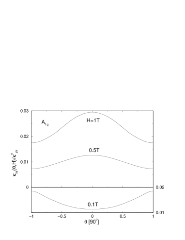
Figure 8: Left panel: Thermal conductivity as function of field angle for type II gap function at various field strengths. This behaviour, notably the sign change of the oscillation amplitude with increasing field corresponds to experimental observations for fields H $\leq$ 2T in Watanabe et al. (2004). Type I,III gap functions (not shown here) exhibit very similar oscillations as shown in the case of ZEDOS (Fig. 6). Right panel: Thermal conductivity for the hybrid (type IV) gap function $\Delta$(k)= $\Delta\cos 2ck_{z}$. A sharp minimum at intermediate $\theta\simeq 51^{\circ}$ due to off-symmetry nodal plane appears. This behaviour is in contradiction to experimental observations Watanabe et al. (2004).

The situation however is different for the hybrid A${}_{1g}\otimes$A’_1g gap function (type IV) which has node lines in non-symmetry planes. The corresponding angle dependence of the thermal conductivity $\kappa_{xx}(\theta)$ is shown in the right panel of Fig. 8. It has a completely different appearance from those for the type I-III gap functions. Firstly, they do not drop to a small value for field angle $\theta=\pm 90^{\circ}$, instead they are even larger than for $\theta$=0. Secondly a pronounced and sharp minimum appears at an intermediate angle $\theta\simeq 51^{\circ}$. This is due to the existence of a non-symmetry nodal plane for the A${}_{1g}\otimes$A’_1g order parameter. In such case both v_x,y(k_z) and v_z(k_z) are nonzero and they give contributions to the DS in Eq. (12) which decrease or increase as function of $\theta$ respectively, leading to the minimum at an intermediate value that survives in the averaged quantities like thermal conductivity. The minimum cannot be discussed away by including the contribution from other FS parts. Firstly it is known from LDA calculations Zwicknagl et al. (2003) that the cylinder FS gives one of the dominant contributions to the total DOS, secondly the other, e.g. ellipisoidal sheets also have a finite v_z at a non-symmetry nodal plane and therefore would give a similar behaviour. Consequently, if the gap function is of the type IV the kink-like minimum at intermediate $\theta$ has to be present in $\kappa_{xx}(\theta)$. However, as mentioned above, the experiments Watanabe et al. (2004) show that it behaves very much as expected for the type I-III gap functions discussed before (Fig. 8, left panel). No trace of a minimum or only depression at intermediate angles has been found. Therefore one has to conclude that the experiments in Watanabe et al. (2004) rule out the type IV gap function $\Delta$(k)=$\Delta\cos(2ck_{z}$) proposed in Won et al. (2004) for UPd₂Al₃. It was already suggested before that in any case this is an unlikely candidate because it is a hybrid gap function with nodes at non-symmetry planes, which has never been found in any other unconventional superconductor.

VII Summary and Outlook

In this work we have investigated the ZEDOS, specific heat and magnetothermal transport properties of superconducting UPd₂Al₃ in the vortex phase using the Doppler shift approximation. Our intention was to give a quantitative basis to the qualitative discussion of possible gap function symmetries presented together with the experimental results of Watanabe et al. (2004). We have given a coherent presentation of the known Doppler shift analysis and expressions and performed the evaluation of physical quantities in a fully numerical approach which allows quantitative predictions. The DS approach is oversimplified in the sense that it does not correctly account for the vortex core contributions and the effect of vortex overlap on approaching H_c2. Therefore one is limited to fields reasonably well below H_c2 but still large enough for the superclean limit to hold. On the other hand it has the great advantage as compared to more advanced semiclassical methods that transport quantities and not only the quasiparticle DOS are easily accessible within a linear response treatment. We have made predictions for the candidate type I-IV gap functions of UPd₂Al₃ which have all line nodes parallel to the hexagonal plane but with different multiplicity and position along k_z. Our quantitative analysis fully confirms the qualitative conjectures drawn in Watanabe et al. (2004). Only gap functions which have nodal lines in symmetry planes containing the BZ boundary or center are compatible with experimental results, those with nodal lines in off-symmetry planes can clearly be ruled out. It was suggested that the nonmonotonic behaviour of the low-field thermal conductivity may be caused by the sensitivity of the effective life time to deviations from unitary scattering. This is also connected with the sign change of the oscillation amplitude for small fields.

The angular-resolved thermal conductivity thus proves that a node line of $\Delta$(k) must be present in a hexagonal symmetry plane, however by itself it cannot distinguish between the possible gap functions of type I-III. As explained in Watanabe et al. (2004) one needs additional information: Inelastic neutron scattering Bernhoeft (2000) requires the translation symmetry $\Delta({\bf k}+{\bf Q})$ = -$\Delta$(k) which would exclude A’_1u, also this gap function is disfavored in Eliashberg theory McHale et al. (2004). Furthermore naive interpretation of Knight shift results Tou et al. (1995) advocates for an even parity gap function, although a comparitive analysis for the A_1g and A_1u states has not been performed McHale et al. (2004) yet. This finally led to the suggestion Watanabe et al. (2004) that the A_1g gap function in the second row of Table 1 is the proper one for UPd₂Al₃.

Presently we have restricted ourselves to gap functions $\Delta(\tilde{\vartheta})$ that have cylindrical symmetry. Our numerical method can straightforwardly be applied to fully anisotropic gap functions $\Delta(\tilde{\vartheta},\tilde{\varphi})$. The calculation then provides us with a direct mapping of $\Delta(\tilde{\vartheta},\tilde{\varphi})\rightarrow\gamma(\theta_{H},\phi_{H})$ or $\kappa_{ii}(\theta_{H},\phi_{H})$ between the momentum dependence of gap functions and the field-angle dependence of physical quantities in their respective 2D domains. Of course this mapping has no unique inverse, but nevertheless comparison with the experimental $\theta_{H},\phi_{H}$- dependence may provide important clues on the anisotropy character of the gap functions. In addition, an extension of the present quantitative theory to different types of FS sheets like FS ellipsoids, corrugated tight binding with FS nesting features etc. is easily possible. Finally we note that the numerical approach to the DS theory may in principle be generalised beyond the perturbative treatment of scattering, i.e. from the superclean to the clean limit with $\Delta|x|<\Gamma\ll\Delta$, although this would likely mean a much larger computational effort.

Appendix A Quasiparticle velocities for corrugated cylindrical FS

In this appendix we define the geometric features and quasiparticle properties of the corrugated cylindrical Fermi surface (FS) which is necessary for the calculation of the Doppler shift energies. Specifically we give the quasiparticle velocities in terms cylindrical coordinates. The corrugated cylinder is the most prominent heavy FS sheet in UPd₂Al₃ obtained in LDA calculations Knöpfle et al. (1996); Inada et al. (1999), dual model calculations Zwicknagl et al. (2003) and also from dHvA experiments Inada et al. (1999). The latter show it has also among the heaviest quasiparticle masses. In the AF BZ ($-\frac{\pi}{\tilde{c}}\leq k_{z}\leq\frac{\pi}{\tilde{c}}$) with $\tilde{c}$ = 2c appropriate for UPd₂Al₃ it can be modeled as

$$\epsilon({\bf k})=\epsilon_{a}({\bf k})-2t_{c}\cos\tilde{c}k_{z}\qquad,\qquad\epsilon_{a}({\bf k})=\frac{\hbar^{2}}{2m_{a}}(k_{x}^{2}+k_{y}^{2})$$ (26)

where the first part is the parabolic ab-plane dispersion and the second part is the tight-binding like dispersion which determines the FS corrugation along c. The diameter of the corrugated cylinder is given by

$$k_{F}^{a}(k_{z})=k_{F}^{0}[1+\frac{2t_{c}}{\epsilon_{F}}\cos(\tilde{c}k_{z})]^{\frac{1}{2}}\qquad;\qquad k_{F}^{0}=\bigl{(}\frac{2m_{a}\epsilon_{F}}{\hbar}\bigr{)}^{\frac{1}{2}}$$ (27)

We introduce the FS corrugation parameter by

$$\gamma_{c}=\frac{k_{F}^{a}(0)}{k_{F}^{a}(\frac{\pi}{\tilde{c}})}\qquad;\qquad\lambda=\frac{2t_{c}}{\epsilon_{F}}$$ (28)

where $\gamma_{c}$ is the ratio of FS cross sectional areas at the (AF) zone center and zone boundary respectively. It is given by

$$\gamma_{c}=\frac{1+\lambda}{1-\lambda}\qquad\mbox{or}\qquad\lambda=\frac{\gamma_{c}-1}{\gamma_{c}+1}$$ (29)

The quasiparticle velocities v_k = $\frac{1}{\hbar}\nabla\epsilon_{{\bf k}}$ in cylindrical coordinates are given by

$$v_{x}(k_{z},\tilde{\varphi}) = v_{a}^{0}\hat{v}_{a}(k_{z})\cos\tilde{\varphi}$$

$$v_{y}(k_{z},\tilde{\varphi}) = v_{a}^{0}\hat{v}_{a}(k_{z})\sin\tilde{\varphi}$$

$$v_{z}(k_{z}) = v_{c}^{0}\hat{v}_{c}(k_{z})$$

$$v_{a}^{0} = \hbar k_{F}^{0}/m_{a}$$ (30)

$$v_{c}^{0} = 2\pi t_{c}/\hbar\tilde{Q}$$

$$\hat{v}_{a}(k_{z}) = [1+\lambda\cos\tilde{c}k_{z}]^{\frac{1}{2}}$$

$$\hat{v}_{c}(k_{z}) = \sin\tilde{c}k_{z}$$

the anisotropy ratio of the Fermi velocity of quasiparticles is then given by ($\tilde{Q}\equiv\frac{\pi}{\tilde{c}}$):

$$\alpha=\bigl{(}\frac{v_{c}^{0}}{v_{a}^{0}}\bigr{)}^{2}=\frac{\pi^{2}}{4}\bigl{(}\frac{k_{F}^{0}}{\tilde{Q}}\bigr{)}^{2}\lambda^{2}\qquad\mbox{or}\qquad\alpha=\frac{\pi^{2}}{4}\bigl{(}\frac{k_{F}^{0}}{\tilde{Q}}\bigr{)}^{2}\bigl{(}\frac{\gamma_{c}-1}{\gamma_{c}+1}\bigr{)}^{2}$$ (31)

The anisotropy ratio $\alpha$ and corrugation factor $\gamma_{c}$ are the parameters which determine the Doppler shift energy for the present FS. The relation between $\alpha$ and $\gamma_{c}$ in Eq. (31) is valid only for parabolic in-plane dispersion. It is better to assume these parameters as independent and take their values from experiment, keeping in mind that $\alpha\rightarrow$ 0 for $\gamma_{c}\rightarrow$ 1.

Finally the FS averages over quasiparticle velocities are given by

$$\langle v^{2}_{\parallel}\rangle_{FS} = \langle v_{x}^{2}+v_{y}^{2}\rangle_{FS}=(v_{a}^{0})^{2}$$

$$\langle v_{z}^{2}\rangle_{FS} = \frac{1}{2}(v_{c}^{0})^{2}$$ (32)

$$\frac{\langle v_{z}^{2}\rangle_{FS}}{\langle v^{2}_{\parallel}\rangle_{FS}} = \frac{1}{2}\alpha$$

Appendix B Critical fields, coherence length penetration depth in uniaxial superconductors

The theory of critical fields H_c1 and H_c2 in superconductors with uniaxial symmetry like D_4h and D_6h was given in Balatskii et al. (1986); Bulaevskii (1990) (see also Abrikosov (1988)) on the basis of Ginzburg-Landau theory for a single component SC order parameter. Here we give a summary of relations derived in these references which are important in our context of Doppler shift calculations. In uniaxial geometry shown in Fig. 1 coherence length and penetration depth are different for fields directed along a or c crystal axes. As a consequence, for intermediate polar field angle $\theta_{H}$ (with respect to c) in the range $0\leq\theta_{H}\leq\frac{\pi}{2}$ the field ($\theta_{H}$) and vortex ($\theta$) directions are not the same. This is an essential difference to the isotropic case where field and vortices are alligned. For uniaxial effective masses m_a, m_c these angles are related by

$$\theta=\tan^{-1}(\frac{1}{\alpha}\tan\theta_{H})\quad;\quad\theta_{H}=\tan^{-1}(\alpha\tan\theta)\quad;\quad\alpha=\frac{m_{a}}{m_{c}}=\bigl{(}\frac{v_{c}^{0}}{v_{a}^{0}}\bigr{)}^{2}$$ (33)

where we assume the convention $-\frac{\pi}{2}\leq\theta,\theta_{H}\leq\frac{\pi}{2}$ for the vortex and field direction. The function $\theta(\theta_{H})$ is plotted in the inset of Fig. 2 for the effective mass anisotropy $\alpha=0.69$ which is the appropriate average value for UPd₂Al₃. For $\alpha$-values only moderately different from one, $\theta$ and $\theta_{H}$ are rather close. However, for $\alpha\ll 1$ the vortices ($\theta$) are ’pinned’ along the c-axis and they are lagging behind the field direction ($\theta_{H}$) when it is continuously changed from c to a. The direction dependence of critical fields is given by

$$H_{c2}(\theta_{H}) = \frac{\Phi_{0}}{2\pi\xi^{2}}\quad;\quad\Phi_{0}=\frac{hc}{2e}$$

$$H_{c1}(\theta_{H}) = \Bigl{[}\frac{H^{a}_{c1}H^{c}_{c1}}{[(H^{a}_{c1})^{2}\cos\theta+(H^{c}_{c1})^{2}\sin\theta]}\Bigr{]}^{\frac{1}{2}}\quad;\quad\theta=\theta(\theta_{H})$$ (34)

Where $\xi$ is given in Eq. 37 and the uniaxial H${}_{c1}^{a,c}$ are obtained from

$$H^{c}_{c1}=\frac{\Phi_{0}}{2\pi}\frac{\ln\kappa_{a}}{\lambda_{a}^{2}}\quad;\quad H^{a}_{c1}=\frac{\Phi_{0}}{2\pi}\frac{\ln(\kappa_{a}\kappa_{c})^{\frac{1}{2}}}{\lambda_{a}\lambda_{c}}\quad\mbox{with}\quad\kappa_{a,c}=\frac{\lambda_{a,c}}{\xi_{a,c}}$$ (35)

The uniaxial Ginzburg-Landau coherence lengths $\xi_{a,c}$ and penetration depths $\lambda_{a,c}$ are given by (i = a,c)

$$\xi_{i}^{2}=\frac{\hbar^{2}\langle v_{i}^{2}\rangle_{FS}}{(kT_{c})^{2}|\tau|}\quad\mbox{and}\quad\lambda_{i}^{2}=\frac{m_{i}c^{2}}{8\pi n_{s}(\tau)e^{2}}$$ (36)

with $\tau$=1-T/T_c. The FS averages for the corrugated cylindrical FS are derived in App. A. The effective field-angle ($\theta_{H}$) dependent coherence length $\xi$ in Eq. (34), penetration depth $\lambda$ and mass m are given by ($\lambda_{\parallel}\equiv\lambda_{a},\xi_{\parallel}\equiv\xi_{a},m_{\parallel}\equiv m_{a}$)

$$\xi=(\xi_{\parallel}\xi_{\theta})^{\frac{1}{2}},\quad\lambda=(\lambda_{\parallel}\lambda_{\theta})^{\frac{1}{2}},\quad m=(m_{\parallel}m_{\theta})^{\frac{1}{2}}$$ (37)

where we used the definitions

$$\xi^{2}_{\theta} = \xi_{a}^{2}\cos^{2}\theta+\xi_{c}^{2}\sin^{2}\theta$$

$$\lambda^{2}_{\theta} = \lambda_{a}^{2}\cos^{2}\theta+\lambda_{c}^{2}\sin^{2}\theta=\frac{m_{\theta}c^{2}}{8\pi n_{s}e^{2}}$$ (38)

$$m_{\theta} = m_{a}\cos^{2}\theta+m_{c}\sin^{2}\theta$$

Note that $\theta$ is the vortex angle with respect to the c-axis which is related to the field angle $\theta_{H}$ via Eq. (33). From the above equations we derive the relations

$$\frac{\lambda_{\parallel}}{\lambda} = \bigl{(}\frac{\lambda_{\parallel}}{\lambda_{\theta}}\bigr{)}^{\frac{1}{2}}=\alpha^{\frac{1}{4}}[\sin^{2}\theta+\alpha\cos^{2}\theta]^{-\frac{1}{4}}$$

$$\frac{\lambda_{\theta}}{\lambda} = \bigl{(}\frac{\lambda_{\theta}}{\lambda_{\parallel}}\bigr{)}^{\frac{1}{2}}=\alpha^{-\frac{1}{4}}[\sin^{2}\theta+\alpha\cos^{2}\theta]^{\frac{1}{4}}$$ (40)

which enter directly the expressions for the Doppler shift energies in Eq. (13).

References

- Sigrist and Ueda (1991) M. Sigrist and K. Ueda, Rev. Mod. Phys. 63, 239 (1991).
- Thalmeier and Zwicknagl (2004) P. Thalmeier and G. Zwicknagl, Handbook on the Physics and Chemistry of Rare Earths (cond-mat/0312540) (Elsevier, 2004), vol. 34, chap. 219, p. 135.
- Volovik and Gor’kov (1985) G. E. Volovik and L. P. Gor’kov, Sov. Phys. JETP 61, 843 (1985).
- Mineev and Samokhin (1999) V. P. Mineev and K. V. Samokhin, Introduction to Unconventional Superconductivity (Gordon and Breach Science Publishers, 1999).
- Joynt and Taillefer (2002) R. Joynt and L. Taillefer, Rev. Mod. Phys. 74, 235 (2002).
- Izawa et al. (2002a) K. Izawa, H. Yamaguchi, T. Sasaki, and Y. Matsuda, Phys. Rev. Lett. 88, 027002 (2002a).
- Izawa et al. (2001a) K. Izawa, H. Takahashi, H. Yamaguchi, Y. Matsuda, M. Suzuki, T. Sasaki, T. Fukase, Y. Yoshida, R. Settai, and Y. Onuki, Phys. Rev. Lett. 86, 2653 (2001a).
- Izawa et al. (2002b) K. Izawa, K. Kamata, Y. Nakajima, Y. Matsuda, T. Watanabe, M. Nohara, H. Takagi, P. Thalmeier, and K. Maki, Phys. Rev. Lett. 89, 137006 (2002b).
- Park et al. (2003) T. Park, M. B. Salamon, E. M. Choi, H. J. Kim, and S.-I. Lee, Phys. Rev. Lett. 90, 177001 (2003).
- Izawa et al. (2001b) K. Izawa, H. Yamaguchi, Y. Matsuda, H. Shishido, R. Settai, and Y. Onuki, Phys. Rev. Lett. 87, 057002 (2001b).
- Izawa et al. (2003) K. Izawa, Y. Nakajima, J. Goryo, Y. Matsuda, S. Osaki, H. Sugawara, H. Sato, P. Thalmeier, and K. Maki, Phys. Rev. Lett. 90, 117001 (2003).
- Aoki et al. (2004) H. Aoki, T. Sakakibara, H. Shishido, R. Settai, Y. Onuki, P. Miranovic, and K. Machida, J. Phys. Condens. Matter 16, L13 (2004).
- Volovik (1993) G. E. Volovik, JETP Lett. 58, 469 (1993).
- Watanabe et al. (2004) T. Watanabe, K. Izawa, Y. Kasahara, Y. Haga, Y. Onuki, P. Thalmeier, K. Maki, and Y. Matsuda, Phys. Rev. B 70, 184502 (2004).
- Geibel et al. (1991) C. Geibel, C. Schank, S. Thies, H. Kitazawa, C. D. Bredl, A. Böhm, M. Rau, A. Grauel, R. Caspary, R. Helfrich, et al., Z. Phys.. B 84, 1 (1991).
- Zwicknagl et al. (2003) G. Zwicknagl, A. Yaresko, and P. Fulde, Phys. Rev. B 68, 052508 (2003).
- Bernhoeft (2000) N. Bernhoeft, Eur. Phys. J. B 13, 685 (2000).
- Sato et al. (2001) N. K. Sato, N. Aso, K. Miyake, R. Shiina, P. Thalmeier, G. Varelogiannis, C. Geibel, F. Steglich, P. Fulde, and T. Komatsubara, Nature 410, 340 (2001).
- Jourdan et al. (1999) M. Jourdan, M. Huth, and H. Adrian, Nature 398, 47 (1999).
- Thalmeier (2002) P. Thalmeier, Eur. Phys. J. B 27, 29 (2002).
- McHale et al. (2004) P. McHale, P. Fulde, and P. Thalmeier, Phys. Rev. B. 70, 014513 (2004).
- Kitaoka et al. (2000) Y. Kitaoka, H. Tou, K. Ishida, N. Kimura, Y. Onuki, E. Yamamoto, Y. Haga, and K. Maezawa, Physica B 281 & 282, 878 (2000).
- Hessert et al. (1997) J. Hessert, M. Huth, M. Jourdan, H. Adrian, C. T. Rieck, and K. Scharnberg, Physica B 230-232, 373 (1997).
- Nishikawa and Yamada (2002) Y. Nishikawa and K. Yamada, J. Phys. Soc. Jpn. 71, 237 (2002).
- Oppeneer and Varelogiannis (2003) P. M. Oppeneer and G. Varelogiannis, Phys. Rev. B 68, 214512 (2003).
- Thalmeier and Maki (2002) P. Thalmeier and K. Maki, Europhys. Lett. 58, 119 (2002).
- Balatskii et al. (1986) A. V. Balatskii, L. I. Burlachkov, and L. P. Gorkov, Sov. Phys. JETP 63, 866 (1986).
- Bulaevskii (1990) L. N. Bulaevskii, Int. J. Mod. Phys. B 4, 1849 (1990).
- Volovik (2004) G. E. Volovik, The Universe in a Helium Droplet (Oxford University Press, 2004).
- Barash et al. (1997) Y. S. Barash, A. A. Svidzinskii, and V. P. Mineev, JETP Lett. 65, 638 (1997).
- Kübert and Hirschfeld (1998) C. Kübert and P. J. Hirschfeld, Solid State Commun. 105, 459 (1998).
- Vekhter et al. (2001) I. Vekhter, P. J. Hirschfeld, and E. J. Nicol, Phys. Rev. B 64, 064513 (2001).
- Won and Maki (2000) H. Won and K. Maki, cond-mat/004105 (2000).
- Dahm et al. (2000) T. Dahm, K. Maki, and H. Won, cond-mat/006301 (2000).
- Won and Maki (2001a) H. Won and K. Maki, Vortices in Unconventional Superconductors and Superfluids (Springer, Berlin, 2001a).
- Won and Maki (2001b) H. Won and K. Maki, Europhysics Letters 56, 729 (2001b).
- Dahm et al. (2002) T. Dahm, S. Graser, C. Iniotakis, and N. Schopohl, Phys. Rev. B 66, 144515 (2002).
- Udagwa et al. (2004) M. . Udagwa, Y. Yanase, and M. Ogata, cond-mat/0408643 (2004).
- Ambegaokar and Griffin (1965) V. Ambegaokar and A. Griffin, Phys. Rev. 137, A1151 (1965).
- Barash and Svidzinskii (1998) Y. S. Barash and A. A. Svidzinskii, Phys. Rev. B 58, 6476 (1998).
- Won et al. (2004) H. Won, D. Parker, K. Maki, T. Watanabe, K. Izawa, and Y. Matsuda, Phys. Rev. B 70, 140509(R) (2004).
- Tou et al. (1995) H. Tou, Y. Kitaoka, K. Asayama, C. Geibel, C. Schank, and F. Steglich, J. Phys. Soc. Jpn. 64, 725 (1995).
- Knöpfle et al. (1996) K. Knöpfle, A. Mavromaras, L. M. Sandratskii, and J. Kübler, J. Phys. Condens. Matter 8, 901 (1996).
- Inada et al. (1999) Y. Inada, H. Yamagami, Y. Haga, K. Sakurai, Y. Tokiwa, T. Honma, E. Yamamoto, Y. Onuki, and T. Yanagisawa, J. Phys. Soc. Jpn. 68, 3643 (1999).
- Abrikosov (1988) A. A. Abrikosov, Fundamentals of the Theory of Metals (North Holland, 1988).