Monte Carlo simulations of liquid crystals near rough walls

Abstract

The effect of surface roughness on the structure of liquid crystalline fluids near solid substrates is studied by Monte Carlo simulations. The liquid crystal is modelled as a fluid of soft ellipsoidal molecules and the substrate is modelled as a hard wall that excludes the centres of mass of the fluid molecules. Surface roughness is introduced by embedding a number of molecules with random positions and orientations within the wall. It is found that the density and order near the wall are reduced as the wall becomes rougher (i.e. the number of embedded molecules is increased). Anchoring coefficients are determined from fluctuations in the reciprocal space order tensor. It is found that the anchoring strength decreases with increasing surface roughness.

I Introduction

The interaction between liquid crystalline (LC) fluids and solid surfaces has attracted much interest Jerome (1992). The presence of the surface breaks the symmetry of the LC phase. As well as being intrinsically interesting this is technologically important - many applications of liquid crystals depend on the interaction between the fluid and an external field, strongly influenced by coupling with external surfaces.

Most previous studies of LC surface anchoring have assumed that the surface is homogenous. Two models are commonly used. In the first the wall is modelled by a perfect crystalline arrayGruhn and Schoen (1998). The second, more coarse grained model, uses an external potential function that depends only on the distance from the wall Wall and Cleaver (1997); Cheung and Schmid (2004). While attractive from a theoretical standpoint, it has long been recognised that deviations from these ideal surfaces can affect the properties of the surface Langmuir (1918). One notable example of this is the reduction of the order parameter of nematic liquid crystals at SiO surfacesBarberi and Durand (1990); Papanek and Martinot-Lagarde (1996). This contrasts with measurements made on other surfacesJerome (1992) (e.g. rubbed polyimide) and with most simulation and theoretical studies that give a higher order parameter at the LC-solid interface. Electron micrographs show that SiO surfaces are extremely roughMonkade et al. (1997), which gives rise to the disordering effect of the surface.

In this paper the structures of nematic and isotropic fluids near rough walls are studied. The effect of roughness is incorporated by embedding a number of molecules in an otherwise smooth wall. These are placed and orientated randomly. Similar models have been used for simple fluids Tang and Harris (1995); Delattre and Dong (1999) and it is hoped that this simple model may give insights into the behaviour of molecular fluids near rough or porous surfaces. Two aspects of the effect of the surface roughness on the LC fluid are studied. Firstly the change in the structure of the fluid was examined. Secondly the effect of surface roughness on the anchoring properties of the LC. The contribution of this surface anchoring to the free energy is often taken to be of the Rapini-Popoular formRapini and Papoular (1969)

$$F_{surf}=W\sin^{2}(\theta-\theta_{0})$$ (1)

where $\theta-\theta_{0}$ is the angle between the director at the surface and the surface’s ’easy-axis’. $W$ is the surface anchoring coefficient. This depends on both the properties of the bulk liquid crystal and on the interaction between the liquid crystal and the surface, so may be expected to vary with surface roughness. As this is a key property in applications of liquid crystals it would be interesting to see how this is affected by changes in the surface morphology.

This paper is organised as follows. Details of the simulation, including the method used for calculating the anchoring coefficient, are given in the next section. The structure of the fluid confined between rough walls is given in Sec. III while results for the anchoring coefficient are presented in Sec. IV. Finally some concluding remarks are given in Sec. V.

II Simulation

II.1 Simulated Systems

In order to simulate large systems, a simple intermolecular potential is used. This models the fluid as a system of soft ellipsoidal molecules interacting through a simplified version of the popular Gay-Berne (GB) potential Gay and Berne (1981). In particular this has two major simplifications. First the orientation dependence of the energy parameter is suppressed. Secondly the potential is cut off and shifted at the potential minima. These changes lead to a much simplier phase diagram than the GB potential, showing only nematic and isotropic phases, closer to the phase behaviour of the hard ellipsoid Frenkel and Mulder (1985) or hard gaussian overlap de Miguel and del Rio (2001) potentials. This potential is also more computationally efficient than the full GB potential.

The interaction between two molecules $i$ and $j$, with positions $\mathbf{r}_{i}$ and $\mathbf{r}_{j}$, and orientations $\mathbf{u}_{i}$ and $\mathbf{u}_{j}$ is given by

$$V(\mathbf{r}_{ij},\mathbf{u}_{i},\mathbf{u}_{j})=\left\{\begin{array}[]{c @{,\:\:} c}4\epsilon_{0}\left[\rho^{-12}-\rho^{-6}\right]+1\hfil,\>\>&\rho\leq 2^{1/6}\\ 0\hfil,\>\>&\mbox{otherwise}\end{array}\right.$$ (2)

where $\epsilon_{0}$ is the energy unit, $\mathbf{r}_{ij}=\mathbf{r}_{i}-\mathbf{r}_{j}$, and

$$\rho(\mathbf{r}_{ij},\mathbf{u}_{i},\mathbf{u}_{j})=\frac{r_{ij}-\sigma(\hat{\mathbf{r}}_{ij},\mathbf{u}_{i},\mathbf{u}_{j})+\sigma_{0}}{\sigma_{0}}.$$ (3)

$r_{ij}=|\mathbf{r}_{ij}|$, $\hat{\mathbf{r}}_{ij}=\mathbf{r}_{ij}/r_{ij}$, and $\sigma_{0}$ is the $\sigma(\hat{\mathbf{r}}_{ij},\mathbf{u}_{i},\mathbf{u}_{j})$ is the shape function given by Berne and Pechukas (1975)

$$\sigma(\hat{\mathbf{r}}_{ij},\mathbf{u}_{i},\mathbf{u}_{j}) = \sigma_{0}\left\{1-\frac{\chi}{2}\left[\frac{(\hat{\mathbf{r}}_{ij}.\mathbf{u}_{i}+\hat{\mathbf{r}}_{ij}.\mathbf{u}_{j})^{2}}{1+\chi\mathbf{u}_{i}.\mathbf{u}_{j}}\right.\right.$$ (4)

$$+\left.\left.\frac{(\hat{\mathbf{r}}_{ij}.\mathbf{u}_{i}-\hat{\mathbf{r}}_{ij}.\mathbf{u}_{j})^{2}}{1-\chi\mathbf{u}_{i}.\mathbf{u}_{j}}\right]\right\}^{-1/2}.$$

This approximates the contact distance between two ellipsoids. In Eq. 4 $\chi=(\kappa^{2}-1)/(\kappa^{2}+1)$ is the anisotropy parameter, where $\kappa$ is the elongation (for the molecules studied here $\kappa=3$).

The wall is represented by a hard core potential acting upon the centres of mass of the molecules. Previous studies have shown that this gives rise to homeotropic alignment at the wall Allen (1999). Roughness is introduced by embedding a number of molecules, $N_{w}$ in the wall. These were given random positions and orientations which were kept fixed during the simulations. While generating these surface configurations interactions between the surface molecules were ignored, thus these molecules may overlap. It should be noted that these molecules do not correspond to real molecules, rather they are used as a convient way of introducing inhomogenity into the wall.The roughness of the wall was characterised by the surface density of these embedded molecules $\Sigma=N_{w}/A$. Some example wall structures are shown in Fig. 1. To ensure some sampling of surface configurations three different surfaces were studied for each pair of $\rho$ and $\Sigma$.

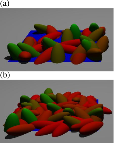
Figure 1: (Color online) Example rough wall configurations for (a) $\Sigma=0.2$ and (b) $\Sigma=0.4$.

Simulations were performed at two average densities, $\rho=0.314$ and $\rho=0.30$. For the higher density the fluid confined between smooth walls was nematic, while it is isotropic for the lower density. The simulated systems were composed of 1200 fluid molecules and up to 63 molecules embedded in each wall. Throughout this reduced units defined by the molecular width $\sigma_{0}$ and the energy unit $\epsilon_{0}$ are used. A reduced temperature of 0.5 was used for both densities.

II.2 Simulation observables

The orientational order may be characterised by the usual nematic order parameter. This is given by the largest eigenvalue of the ordering tensor, defined as

$$Q_{\alpha\beta}=\frac{1}{N}\sum_{i=1}^{N}\left(\frac{3}{2}u_{i\alpha}u_{i\beta}-\frac{1}{2}\delta_{\alpha\beta}\right),~{}~{}\alpha,\beta=x,y,z$$ (5)

where $\mathbf{u}_{i}$ is the orientation of the $i$th molecule and $\delta_{\alpha\beta}$ is the Kronecker delta function. It may also be informative to consider the order parameter in the cell bulk and near the surface, $S^{bulk}$ and $S^{surf}$. $S^{bulk}$ is calculated for molecules within the region $l_{z}/4\leq z\leq 3l_{z}/4$, while $S^{surf}$ is calculated for molecules within 1 $\sigma_{0}$ of the surface.

The distribution of molecules in the simulation cell can be described by the density profile $\rho(z)$. To describe the ordering through the cell, the ordering tensor Eq. 5 can be calculated throughout the cell. Diagonalising this gives the order parameter profiles ($q_{+}(z)$, $q_{0}(z)$, and $q_{-}(z)$). These can be expressed as $S(z)$, $S(z)+\frac{1}{2}S_{xy}(z)$, and $S(z)-\frac{1}{2}S_{xy}(z)$, where $S(z)$ is the nematic order parameter and $S_{xy}(z)$ is the biaxiality parameter.

The nematic director $\mathbf{n}(z)$ can be identified with the eigenvector of the ordering tensor corresponding to the largest eigenvalue.

While the presence of layers may be deduced from the density profiles it may be useful to quantify the degree of translational order. The smectic order parameter may be introduced for this purpose Steuer et al. (2004); Bates and Luckhurst (1999). This is given by

$$\rho_{1}=\left<\left|\frac{1}{N}\sum_{j=1}^{N}\exp\left(\frac{2\pi iz_{j}}{d}\right)\right|\right>,$$ (6)

where $d$ is the layer periodicity. This is initially unknown and is take to be the value that maximises $\rho_{1}$ Bates and Luckhurst (1999).

II.3 Director fluctuations and surface anchoring

The surface anchoring coefficient is determined by the director fluctuation method Andrienko et al. (2000); Andrienko and Allen (2002). This method relates thermal director fluctuations in a confined geometry to the zenithal anchoring coefficient, in a similar manner as the fluctuations in a bulk LC can be related to the bulk elastic constants Forster (1975); Allen et al. (1996). The theory for this has been extensively developed elsewhere and this section will contain only the briefest of outlines.

As for the bulk elastic constants the zenithal anchoring coefficient may be determined by fitting elastic theory predictions of fluctuations in the ordering tensor to those determined from simulations. The reciprocal space ordering tensor is given by

$$Q_{\alpha\beta}(\mathbf{k})=\frac{V}{N}\sum_{j}Q_{\alpha\beta}^{j}\exp\left(i\mathbf{k}.\mathbf{r}_{i}\right).$$ (7)

Fluctuations can be calculated from simulation

$$\left<\left|Q_{\alpha\beta}(k_{z})\right|^{2}\right> = \frac{V^{2}}{N^{2}}\left[\left(\sum_{j}Q_{\alpha\beta}^{j}\cos(k_{z}z_{j})\right)^{2}\right.$$ (8)

$$+\left.\left(\sum_{j}Q_{\alpha\beta}^{j}\sin(k_{z}z_{j})\right)^{2}\right],$$

The corresponding elastic theory predicts that there fluctuations are given by Andrienko et al. (2000)

$$\left<\left|Q_{\alpha\beta}(k_{z})\right|^{2}\right> = \frac{9}{8}k_{B}T\frac{S^{2}V}{K_{33}}\sum_{q_{z}}\frac{\chi^{2}+\zeta^{2}}{q_{z}^{2}(2\zeta+\zeta^{2}+\chi^{2})}\times$$

$$\left|\frac{e^{i(\kappa+\chi)}-1}{\kappa+\chi}+\left(\frac{i\chi-\zeta}{i\chi+\zeta}\right)\frac{e^{i(\kappa-\chi)}-1}{\kappa-\chi}\right|^{2}$$

where $K_{33}$ is the bend elastic constant. $q_{z}$ is a wave vector with a discrete spectrumAndrienko et al. (2000), $\chi=q_{z}L_{e}$, and $\kappa=k_{z}L_{e}$. $\zeta$ is the anchoring strength parameter

$$\zeta=\frac{WL_{e}}{K_{33}}=\frac{L_{e}}{\lambda}$$ (10)

where $W$ is the zenithal anchoring coefficient and $\lambda$ is the extrapolation length. $L_{e}$ is the cell thickness appearing in the elastic theory; this is not necessarily equal to the simulation cell thickness, $L_{z}$. In fitting the elastic theory to simulation profiles $L_{e}$ and $\zeta$ are the fitting parameters. $K_{33}$ has been determined from simulation for a nearby state pointPhoung et al. (2001) ($\rho=0.30$). While this value ($K_{33}=1.48$) is likely to be too large for some of the systems studied here, this should be sufficient for a qualitative study.

III Fluid Structure

III.1 High Density Fluid

The density profiles for the high density fluid are shown in Fig. 2a. The effect of the wall roughness is most apparent near the wall. Here the density near the surface decreases with increasing $\Sigma$. This is caused by the decrease in available volume near the wall due to the embedded molecules. Values of the density near the wall are presented in Tab. III.1. The surface density falls from 0.72 for the smooth wall to 0.34 for the rough wall with $\Sigma=0.4$.

Another noticeable difference is that the second peak (at $z=2.8$ for the plain wall) becomes broader. This arises from the surface disorder disturbing the layer structure and has been observed in simulations of Lennard-Jones fluids Delattre and Dong (1999). This can more clearly be seen in the inset, which shows the detail of the density profiles around the minima. The disruption of the translational ordering caused by the embedded molecules can be seen by considering the smectic order parameter (Eq. 6). Values for these are presented in Tab. III.1. As can be seen $\rho_{1}$ markedly decreases with increasing grafting density, as would be expected for increasing translational disorder.

Figure 2: (a) Density profiles for the high density fluid near rough walls. The density profile for grafting density $\Sigma=0$ is shown by the solid line, for $\Sigma=0.1$ dotted line, $\Sigma=0.2$ dashed line, $\Sigma=0.3$ long dashed line, and $\Sigma=0.4$ the dashed dotted line. Inset shows the density profiles around the minima. Symbols as in main figure.
(b) Order parameter profiles for high density fluid near rough walls. Symbols as in (a).
(c) Biaxiality ($S_{xy}$) profiles for high density fluid near rough wall. Symbols as in (a).
(d) $z$ component of the director for the high density fluid. Symbols as in (a). 3 $n_{z}(z)$ profiles are shown for $\Sigma=0.4$.

Far from the wall the profiles all tend to a constant values, indicating a layer of bulk fluid. The density of this layer increases slightly with increasing grafting density. This arises as the embedded molecules exclude fluid molecules from regions near the wall, increasing the number of molecules in the cell bulk. This is a consequence of having a fixed cell size and may be avoided by using $NpT$ simulations. Quantitively this can be seen by examining the densities in the cell bulk. Values for this are presented in Tab. III.1. The density in the bulk of the cell goes from 0.29 for the smooth wall to 0.31 for the highest grafting densities.

Figure 2(b) shows the order parameter profiles for different values of $\Sigma$. As can be seen the value of the order parameter at the wall is lower for higher grafting densities. This is caused by the disorientating effect of the embedded molecules. This disorientating effect also leads to a deeper minima. For $\Sigma\geq 0.2$ this leads to a small layer (approximately 1 molecular width thick) of almost isotropic fluid. The position of this minima moves closer to the wall with increasing surface roughness. For the smooth wall this minima is at approximately $z=2$, while for the highest grafting densities it appears at about $z=1.1$. Again this is attributable to the disruption in the surface induced layering. As for $\rho(z)$ the second peak becomes broader with increasing $\Sigma$. Finally, as can be seen from Tab. III.1 the bulk order parameter $S^{bulk}$ increases with increasing $\Sigma$. This is a consequence of the increasing density in the centre of the cell due to the excluded volume effect of the embedded molecules. It is noticeable that for $\Sigma\geq 0.2$ $S^{bulk}$ becomes larger than $S^{surf}$.

The biaxiality profiles are shown in Fig. 2(c). For the smooth wall the this is essentially zero (the largest value is 0.04) reflecting the cylindrical symmetry around the $z$ axis. However, for the rough walls there is are sizable peaks in the biaxiality profiles. These are stronger for larger values of $\Sigma$ and are in the region of $0.5\leq z\leq 1.3$, corresponding to regions of low order. This surface induced biaxiality has been seen for simulations of LCs near grooved surfaces Stelzer et al. (1997).

Table 1.

Densities and order parameters for the simulated systems. $\rho_{bulk}$ and $\rho_{surf}$ are the bulk and surface densities, $S$, $S^{bulk}$ and $S^{surf}$ are the total, bulk and surface order parameters, and $\rho_{1}$ is the smectic order parameter. Errors in the last decimal place are in parenthesises.

$\rho$	$\Sigma$	$\rho_{surf}$	$\rho_{bulk}$	$S$	$S^{surf}$	$S^{bulk}$	$\rho_{1}$
0.314	0	0.72(1)	0.286(3)	0.60(3)	0.84(1)	0.53(6)	0.14(2)
0.314	0.1	0.61(1)	0.294(2)	0.64(2)	0.76(2)	0.65(3)	0.12(2)
0.314	0.2	0.48(3)	0.304(3)	0.67(2)	0.65(3)	0.72(2)	0.10(2)
0.314	0.3	0.43(5)	0.308(4)	0.69(2)	0.65(9)	0.75(2)	0.09(2)
0.314	0.4	0.33(2)	0.307(9)	0.66(8)	0.58(7)	0.73(7)	0.07(2)
0.300	0	0.70(1)	0.273(2)	0.28(3)	0.81(1)	0.10(4)	0.14(2)
0.300	0.1	0.59(1)	0.281(2)	0.34(7)	0.72(3)	0.27(9)	0.12(2)
0.300	0.2	0.46(2)	0.291(3)	0.52(6)	0.61(3)	0.59(5)	0.10(2)
0.300	0.3	0.41(2)	0.293(3)	0.51(4)	0.53(9)	0.60(4)	0.09(2)
0.300	0.4	0.38(1)	0.300(3)	0.59(6)	0.54(5)	0.69(3)	0.07(2)

Figure 2(d) shows the $z$ component of the director for each $\Sigma$. In the cell bulk the director is essentially parallel to the $z$ axis. For $\Sigma\geq 0.2$ there is a tilt away from the $z$ axis at about the position of the order minima. As may be expected this is most pronounced for the $\Sigma=0.4$ wall. In Fig. 2d the profiles for each of the $\Sigma=0.4$ walls are shown separately. It can be seen that the size of this tilt differs strongly for different wall configurations (for the largest the tile angle is approximately $79^{\circ}$). For the larger tilt angles this propagates into the bulk of the fluid leading to a director tilted up to $16^{\circ}$ from the $z$-axis. It is not clear how a randomly generated wall gives rise to a titled configuration in the bulk. Similar behaviour has been seen in a recent study of a LC near a planar wall with perpendicularly grafted rodsDowntown and Allen (2004). In that case the bulk tilt was caused by the competition between the wall (which promoted planar alignment) and the embedded molecules. As it appears only for a subset of the walls studied here it would be desirable to consider further wall configurations.

Figure 3: (Color online) Simulation configurations showing molecules within 2.5 $\sigma_{0}$ of the surface for (a) $\Sigma=0$, (b) $\Sigma=0.2$, and (c) $\Sigma=0.4$. For each $\Sigma$ the left most picture shows molecules with $0\leq z\leq 0.5$, the centre pictures shows $0.5\leq z\leq 1.5$, and the right most shows $1.5\leq z\leq 2.5$.

The previous discussion may be illuminated by examination of simulation configurations. Figure 3 shows configurations of for $\Sigma=0.0$ (smooth wall), $\Sigma=0.2$, and $\Sigma=0.4$. The disordering effect of the rough wall can be seen in the first and second layers (left and right most pictures). However, the fluid between these two layers shows the most noticeable change with increasing $\Sigma$. For the smooth wall the molecules in this region are still well ordered parallel to the $z$-axis. With increasing $\Sigma$ the molecules in this region become increasingly disordered. This gives rise to the deeper minima seen in the order parameter profile (Fig. 2(b)). Additionally it can be seen that many of the molecules lie in the $xy$ plane, giving rise to the biaxiality peak and the tilt of the director away from the $z$ axis. This behaviour is similar to that seen in simulations of smectic liquid crystals von Roij et al. (1995) where molecules in the region between the layers are seen to align either parallel or normal to the layers. These planar oriented molecules possibly give rise to the bulk tilt seen in some cases. Finally the number of molecules in this region visibly increases with $\Sigma$.

III.2 Low Density Fluid

Here the density and order parameter profiles for the low density system are discussed. For the smooth wall the density in the bulk of the cell is 0.27 (Tab. III.1), just below the isotropic-nematic transition density for this system ($\rho_{I-N}=0.287$). As the density in the cell bulk increases with $\Sigma$, for $\Sigma\geq 0.2$ the fluid in the cell bulk is nematic rather than isotropic.

The density profiles for the low density fluid are shown in Fig. 4(a). The changes in the density profile with increasing $\Sigma$ are similar to those in the high density system - the density at contact decreases with $\Sigma$ and the second peak becomes more diffuse. Again this can be gleaned from the decrease in the value of the smectic order parameter with $\Sigma$ (Tab. III.1). It is interesting to note that the values of $\rho_{1}$ obtained in this system are very similar to those for the higher density system, indicating the similarity in the structure of both systems.

Figure 4: (a) Density profiles for the low density fluid near rough walls. The density profile for grafting density $\Sigma=0$ is shown by the solid line, for $\Sigma=0.1$ dotted line, $\Sigma=0.2$ dashed line, $\Sigma=0.3$ long dashed line, and $\Sigma=0.4$ the dashed dotted line.
(b) Order parameter profiles for the low density fluid. Symbols as in (a).

Shown in Fig. 4(b) are the order parameter profiles. As in the high density fluid the value of the order parameter at the wall decreases as $\Sigma$ increases. The order parameter profile also shows a deeper minima with increasing surface roughness. It is noticeable that even in this lower density case there is not an appreciable layer of isotropic fluid between the wall and bulk fluid. This has been predicted to happen near rough walls as a consequence of the competition between the bulk director and the local boundary conditions Sluckin (1995).

IV Surface Anchoring

Shown in Fig. 5 are the order tensor fluctuations as a function of wavevector. As can be there is good agreement between the simulation and elastic theory curves, especially for small $k_{z}$.

Figure 5: Order tensor fluctuations (normalised by cell volume) as a function of wavevector for (a) high density and (b) low density fluids. In both graphs the simulation data is denoted by symbols (circles $\Sigma=0$, squares $\Sigma=0.1$, diamonds $\Sigma=0.2$, triangles $\Sigma=0.3$, and crosses $\Sigma=0.4$) and the elastic theory data is shown by lines (continuous line $\Sigma=0$, dotted line $\Sigma=0.1$, dashed line $\Sigma=0.2$, long dashed line $\Sigma=0.3$, and dot dashed line $\Sigma=0.4$). The order tensor fluctuations for $\Sigma=0.0$ are shown only in (a).

The fitted values for the anchoring coefficients are given in Tab. IV along with values of the extrapolation length $\lambda$ and the surface anchoring coefficient $W$. For both bulk densities $\zeta$ tends to decrease with increasing $\Sigma$.

Table 2.

Fitting data for the order tensor fluctuations (Fig. 5). $\zeta$ is the anchoring coefficient, and $L_{e}$ is the elastic theory cell width, which appear in Eq. LABEL:eqn:ordert_fl_elastic. $\lambda=L_{e}/\zeta$ is the extrapolation length and $W=K_{33}/\lambda$ is the surface anchoring strength.

$\rho$	$\Sigma$	$\zeta$	$L_{e}$	$\lambda$	$W$
0.314	0.0	5.62	16.00	2.85	0.52
0.314	0.1	6.51	28.39	4.36	0.34
0.314	0.2	5.64	29.36	5.21	0.28
0.314	0.3	4.94	26.80	5.43	0.27
0.314	0.4	4.55	27.78	6.11	0.24
0.30	0.1	3.05	18.32	6.01	0.24
0.30	0.2	2.88	24.60	8.54	0.17
0.30	0.3	2.58	23.85	9.24	0.16
0.30	0.4	2.70	25.44	9.42	0.16

The behaviour of the elastic theory cell width, $L_{e}$, with $\Sigma$ deserves comment. For the high density fluid, $L_{e}$ for the smooth wall is 16.00 $\sigma_{0}$, a few molecular lengths smaller than the physical cell width ($L_{z}=24.66$). This is similar to behaviour seen in previous simulationsAndrienko et al. (2000); Andrienko and Allen (2002) and is due to the formation of highly ordered layers in the vicinity of the surface. For the rough walls however, $L_{e}$ is larger than $L_{z}$. This increase may be attributable to the rough surface breaking up the highly ordered surface layer. Thus instead of the elastic theory boundary conditions being applied at this layer, they are applied closer to the wall, leading to an increase in $L_{e}$.

For both bulk densities the extrapolation length increases and the anchoring coefficient $W$ decreases with $\Sigma$. Thus, as may be intuitively expected, anchoring on rough surfaces is weaker than on smooth surfaces.

V Summary

In this paper results of Monte Carlo simulations for a confined fluid of ellipsoidal molecules have been performed. The effect of surface roughness on the structure of the fluid has been examined. Roughness was introduced by embedding a number of molecules, with random positions and orientations, in otherwise smooth walls. Increasing the number of molecules embedded in the wall corresponds to an increasing surface roughness. The simulations were performed at two bulk densities. For the higher density the fluid in the bulk of the cell is nematic for the smooth wall case, while for the lower density it is isotropic.

At both densities studied the effect of increasing surface roughness is similar. Both the density and order parameter in the region near the wall decrease as the number of embedded molecules increases. The decrease in the density arises from the excluded volume of the embedded molecules, while the decrease in the order can be attributed to the disorientating effect of the randomly orientated molecules in the wall. The rough walls also act to smear out the secondary peaks in the density and order parameter profiles as the embedded molecules give anchoring points at positions other than at the wall surface. One side effect of the wall roughness is an increase in the density and order parameter in the centre of the cell.

Also studied was the effect of surface roughness on the surface anchoring strength. For both systems the anchoring was found to become progressively weaker with increasing surface roughness.

A number of possible avenues for future work are possible. Calculation of the anchoring coefficient via alternative methodsAllen (1999); Stelzer et al. (1995) would be useful. As the formation of a highly ordered layer at the surface is commonly held to be important for the growth of order in confined liquid crystals, it may be interesting to investigate the effect of wall roughness on the phase behaviour of the confined fluid Steuer et al. (2004). Integral equation Dong et al. (1995) or density function theories Schmidt (2003) have been applied to similar systems of simple fluids and appropriate generalisations to molecular fluids should also prove useful.