Incorporating fluctuations and dynamics in self-consistent field theories for polymer blends

Zusammenfassung

We review various methods to investigate the statics and the dynamics of collective composition fluctuations in dense polymer mixtures within fluctuating-field approaches. The central idea of fluctuating-field theories is to rewrite the partition function of the interacting multi-chain systems in terms of integrals over auxiliary, often complex, fields, which are introduced by means of appropriate Hubbard-Stratonovich transformations. Thermodynamic averages like the average composition and the structure factor can be expressed exactly as averages of these fields. We discuss different analytical and numerical approaches to studying such a theory: The self-consistent field approach solves the integrals over the fluctuating fields in saddle-point approximation. Generalized random phase approximations allow to incorporate Gaussian fluctuations around the saddle point. Field theoretical polymer simulations are used to study the statistical mechanics of the full system with Complex Langevin or Monte Carlo methods. Unfortunately, they are hampered by the presence of a sign problem. In dense system, the latter can be avoided without losing essential physics by invoking a saddle point approximation for the complex field that couples to the total density. This leads to the external potential theory. We investigate the conditions under which this approximation is accurate. Finally, we discuss recent approaches to formulate realistic dynamical time evolution equations for such models. The methods are illustrated by two examples: A study of the fluctuation-induced formation of a polymeric microemulsion in a polymer-copolymer mixture, and a study of early-stage spinodal decomposition in a binary blend.

Index for monomer species ($A$ or $B$)

Index for polymer species (homopolymer $A$, homopolymer $B$, copolymer)

Number of segments of a chain

Flory-Huggins parameter

Volume

Polymer number density

End-to-end distance of a polymer

Invariant degree of polymerization, ${\bar{\cal N}}={\varrho}R_{e}^{d}$.

Volume fraction of polymers of type $J$

Distributions of segments of species $\alpha$ along a polymer of type $J$

Microscopic segment density of species $\alpha$ (Eq. (3))

Complex field-theoretical Hamiltonian as a function of fluctuating fields (Eqs. (10),(11))

Single chain partition function of type $J$ (Eqs. (12),(13))

End-segment distribution (Eqs. (17),(18))

Hamiltonian of the external potential theory (Eqs. (41),(42))

Hamiltonian of the (dynamic) SCF theory (Eq. (53))

Onsager coefficient (Eq. (110))

single chain self-diffusion constant

1 Introduction

Polymeric materials in daily life are generally multicomponent systems. Chemically different polymers are “alloyed” as to design a material which combines the favorable characteristics of the individual components APPLICATION . Understanding the miscibility in the molten state is crucial for understanding and tailoring properties that are relevant for practical applications. Miscibility on a microscopic length scale is desirable, for instance, to increase the tensile strength of the material. Unfortunately, different polymers are typically not microscopically miscible, because the entropy of mixing is much smaller for polymers than for small molecules. The mixture separates into domains in which one of the components is enriched. The domains are separated by interfaces. Tuning the interface tension between the coexisting phases, and the morphology of the material on a mesoscopic length scale, is a key to tailoring material properties and has attracted abiding interest.

One strategy to improve the miscibility and the interfacial properties has been to synthesize copolymers by chemically linking polymers of different type to each other. Added in small amounts to a homopolymer mixture, the copolymers adsorb at the interfaces, change their local structure, and reduce the interfacial tension RUSSELL ; KRAMER ; BUD ; HASHI . Mixtures containing substantial amounts of copolymers form new types of phases, where different monomer types aggregate into mesoscopic “phase separated” domains (microphase separation). By varying the composition of the mixture and the architecture of the individual (co)polymers, one can create a wide range of different morphologies, corresponding to different materials, each with unique material properties.

Unfortunately, copolymers are often rather expensive components. Another, cheaper, strategy for tuning the domain structure of blends takes advantage of the fact that in many practical applications, polymeric blends never reach thermal equilibrium on larger length scales. The morphology of the blend strongly depends on the kinetics of phase separation. Finer dispersed morphologies can be obtained by optimizing the processing conditions jansen ; tucker .

One of the most powerful methods to assess such phenomena theoretically is the self-consistent field (SCF) theory. Originally introduced by Edwards EDWARDS and later Helfand et al. helfand , it has evolved into a versatile tool to describe the structure and thermodynamics of spatially inhomogeneous, dense polymer mixtures hong ; scheutjens ; matsen ; review . The SCF theory models a dense multi-component polymer mixture by an incompressible system of Gaussian chains with short-ranged binary interactions, and solves the statistical mechanics within the mean-field approximation.

Much of the success of the SCF theory can be traced back to the extended size of the polymer molecules:

First,the large size of the chain molecules imparts a rather universal behavior onto dense polymer mixtures, which can be characterized by only a small number of coarse-grained parameters, e. g., the end-to-end distance $R_{e}$ of the molecules, and the incompatibility per chain $\chi N$, where the Flory-Huggins parameter $\chi$ FH describes the repulsion between segments belonging to different components, and $N$ is the number of segments per molecule. $R_{e}$ sets the characteristic length scale of spatial inhomogeneities. Since this length scale is much larger than the size of the repeat units along the backbone of the polymer chain, these systems can be described successfully by coarse-grained chain models. The parameters, $R_{e}$ and $\chi N$, encode the chemical structure of the polymer on microscopic length scales. Indeed, comparisons between the predictions of the SCF theory and experiments or simulations have shown that the properties of many blends on large length scales depend on the atomistic structure only via the coarse-grained parameters $R_{e}$ and $\chi N$. The comparison works best if the parameters $R_{e}$ and $\chi$ are considered as “black box” input parameters. Their determination from first principles or even from a well-defined microscopic model (e. g., atomistic force fields), is a formidable theoretical challenge: Even in the simplest case, the Flory-Huggins parameter $\chi$ stems from small differences of dispersion forces between the different chemical segments. The value of the end-to-end distance $R_{e}$ of a polymer in a homogeneous melt results of a subtle screening of excluded volume interactions along the chain by the surrounding molecules, and $R_{e}$ depends on the density and temperature. Thus $\chi$ and $R_{e}$ cannot be calculated rigorously. If these coarse-grained parameters are determined independently (e. g., by experiments) and used as an input, the SCF theory is successful in making quantitative predictions.

These arguments rationalize the success of a coarse-grained approach. The second reason for the success of a the SCF theory, which is a mean-field theory, is the fact that due to their extended shape, the molecules have many interaction partners. Let ${\varrho}$ denote the polymer number density. The number of molecules inside the volume of a reference chain is then given by $\sqrt{{\bar{\cal N}}}={\varrho}{R_{e}^{d}}$ (where $d$ denotes the spatial dimension). This quantity measures the degree of interdigitation of the molecules. In a dense three dimensional melt, ${{\bar{\cal N}}}$ is proportional to the number of segments $N$ per chain, and it is refered to as the invariant degree of polymerization COMMENT . For systems which differ in ${{\bar{\cal N}}}$ but are characterized by the same $\chi N$ and $R_{e}$ the SCF theory will make identical predictions. The quantity ${{\bar{\cal N}}}$ plays an important role as it controls the strength of fluctuations.

In this contribution, we shall discuss improvements which incorporate fluctuations into the SCF theory. Those fluctuations are particularly important (i) in the vicinity of phase transitions (e. g., the unmixing transition in a binary blend or the onset of microphase separation in block copolymers) or (ii) at interfaces, where the translational symmetry is broken and the local position of the interface can fluctuate. Both type of fluctuations can qualitatively change the behavior compared to the prediction of mean-field theory. The outline of the manuscript is as follows: First we introduce the Edwards model, which is employed as a coarse-grained description of a dense polymer melt throughout the article. Then, we briefly summarize the SCF theory for equilibrium properties and discuss various numerical strategies. Subsequently, we proceed to discuss possibilities to go beyond the mean-field approximation and obtain a description of the dynamics. Finally, we discuss some selected applications and close with a brief outlook on interesting problems.

2 The Edwards model for polymer blends

2.1 Gaussian model

In dense binary blends, many of the interesting phenomena occur on length scales much larger than the size of a monomeric unit. Hence, a theoretical description can use a coarse-grained model, which only incorporates the relevant ingredients that are necessary to bring about the observed universal behavior: chain connectivity and thermal interaction between unlike monomeric units. The universal properties on length scales much larger than the size of a monomeric unit do not depend on the details of these interactions. One can therefore choose a convenient mathematical model, the Edwards Hamiltonian EDWARDS , in which the local microscopic structure enters only via three phenomenological parameters, $R_{e}$, $\chi N$, and ${\bar{\cal N}}$.

In a dense melt, the excluded volume of the monomeric units is screened and chains adopt Gaussian conformations on large length scales. In the following, we shall describe the conformations of a polymer as space curves ${\bf r}(\tau)$, where the contour parameter $\tau$ runs from 0 to 1. The probability distribution ${\mathcal{P}}[{\mathbf{r}}]$ of such a path ${\bf r}(\tau)$ is given by the Wiener measure

$${\mathcal{P}}[{\mathbf{r}}(\tau)]\sim\exp\left[-\frac{3}{2R_{e}^{2}}\int_{0}^{1}d\!\tau\left(\frac{d{\mathbf{r}}}{d\tau}\right)^{2}\right].$$ (1)

This describes the Gaussian chain conformations of a non-interacting chain. It is characterized by a single length scale, $R_{e}$ the end-to-end distance of the polymer chain. The structure is Gaussian on all length scales, i. e., the model ignores the structure on short length scales deGennes : Self-avoiding walk statistics inside the excluded volume blob, rod-like behavior on the length scale of the persistence length, and the details of the monomeric building units at even shorter length scales. All this structure on the microscopic length scale enters the Gaussian chain model only through the single parameter $R_{e}$. This parameter (and its dependence on the thermodynamic state, i. e., temperature, density or pressure) cannot be predicted by the theory but is used as input. The Gaussian model provides an appropriate description if the smallest length scale $l_{\rm min}$ of interest in the calculations is much larger than microscopic length scales. The coarse-graining length scale $l_{\rm min}$ should be at least on the order of a few persistence lengths. If this condition is violated, the Gaussian chain model can produce qualitatively incorrect predictions (e. g., at low temperatures where both the persistence length length becomes large and the interface width becomes small). In this case, other chain models have to be employed that take due account of the local structure (e. g., the worm-like chain model WORM , which captures the crossover from Gaussian conformations at large length scales to rod-like behavior on the length scale of the persistence length, or enumeration schemes SZLEIFER ; MSROD ; LV ; MCONF which can deal with arbitrary chain architecture).

In the following we consider a polymer blend of homopolymers of species $A$ and $B$ and/or copolymers containing both types of monomers. For simplicity, we assume that segments of type $A$ and $B$ are perfectly symmetrical and that all polymers have the same chain characteristics, in particular, the same chain length. The generalization to more asymmetrical situations is straightforward. We characterize the distribution of segments $A$ and $B$ along a chain of given type $J$ (corresponding to a $A$-homopolymer, a $B$-homopolymer or an $A:B$ block copolymer) by the segment occupation functions $\gamma_{JA}(\tau)$, $\gamma_{JB}(\tau)$ MatsenRev , which take the value 0 or 1 and fulfill

$$\gamma_{JA}(\tau)+\gamma_{JB}(\tau)=1\qquad\mbox{for all $J$ and $\tau$}.$$ (2)

Combining these with the chain conformations ${\bf r}(\tau)$, we can define a microscopic density $\hat{\phi}_{\alpha}({\bf r})$ for segments of type $\alpha=A$ or $B$

$$\hat{\phi}_{\alpha}=\frac{1}{{\varrho}}\sum_{J}\sum^{n_{J}}_{i_{J}=1}\int_{0}^{1}{\rm d}\tau\;\delta({\mathbf{r}}-{\mathbf{r}}_{i_{J}}(\tau))\gamma_{J\alpha}(\tau).$$ (3)

Here the sum $i_{J}$ runs over all $n_{J}$ polymers of type $J$, and ${\bf r}_{i_{J}}(\tau)$ denotes the conformation of the $i_{J}^{\rm th}$ polymer. The segment density is normalized by the polymer number density, ${\varrho}\equiv\sum_{J}n_{J}/{\cal V}$.

In addition to the chain connectivity, the coarse-grained model has to capture the interactions between segments. In general, a compressible binary polymer mixture CMIX exhibits both liquid-liquid immiscibility as well as liquid-vapor type phase separation (cf. Polymer+solvent systems: Phase diagrams, interface free energies, and nucleation in this issue). In the following, however, we regard only liquid-liquid unmixing into $A$-rich and $B$-rich phases or microphase separation into domains comparable in size to the molecular extension.

To describe the interaction in the polymer liquid, the interaction potential between segments can be decomposed in a short-ranged repulsive part and a longer-ranged attractive part (e. g., using the Barker-Henderson scheme BH or the Weeks-Chandler-Anderson decomposition HMC ). The short-ranged repulsive contribution determines the packing and structure of the fluid. The length scale of fluctuations in the total density is set by the excluded volume correlation length $\xi_{\rm ev}$, which also sets the length scale below which the chain conformations do not obey Gaussian but rather self-avoiding walk statistics. In a dense melt, $\xi_{\rm ev}$ is a microscopic length scale. On length scales larger than $\xi_{\rm ev}$ density fluctuations have already decayed, i. e., the fluid is incompressible. For $\xi_{\rm ev}\ll l_{\rm min}$, we can represent the effect of the short-ranged repulsive interactions by an incompressibility constraint:

$$\hat{\phi}_{A}({\bf r})+\hat{\phi}_{B}({\bf r})=1$$ (4)

where we have assumed that both segments occupy identical volumes. Of course, this incompressibility constraint can only be enforced after the coarse-graining procedure, i. e., on length scales larger than $\xi_{\rm ev}$. The short-ranged repulsive interactions, hence, do not enter the Edwards Hamiltonian explicitely, but only via the number density of polymers ${\varrho}$. The dependence of ${\varrho}$ on the thermodynamic state (i. e., the temperature, pressure, and composition of the mixture) – the equation of state – is not predicted by this computational scheme.

The longer-ranged attractive interactions between the segments do not strongly influence the local fluid structure, but drive the phase separation. Again we assume that the range of the attractive interactions is small compared to smallest length scale $l_{\rm min}$ of interest in our calculations. Then, the detailed shape of the longer-ranged potential does not matter either, and we can represent the interactions as zero-ranged. By virtue of the incompressibility constraint, there is only one independent bilinear form of densities and so we use as interaction free energy the expression

$$k_{B}T{\varrho}\chi N\int{{\rm d}^{d}{\bf r}}\;\hat{\phi}_{A}({\bf r})\hat{\phi}_{B}({\bf r})$$ (5)

The combination of Flory-Huggins parameter and chain length, $\chi N$, parameterizes all the subtle interplay between liquid-like structure of the polymeric liquid and the small differences in the attractive interactions between segments of different types. It is worth noting that the Flory-Huggins parameter for neutral polymers without specific interactions is on the order $10^{-4}-10^{-2}$ PH , while the strength of the attractive interactions in the fluid are of order 1 $k_{B}T$. Hence the $\chi$ parameter, which describes the difference in attractive interactions between the species, arises from a strong cancellation. Small changes in the thermodynamic state might perturb this balance. As a result, the $\chi$-parameter depends on the temperature, pressure and composition, as is often observed in experiments.

Within the coarse-grained model the canonical partition function of a polymer mixture with $n_{J}$ chains of type $J$ takes the form:

$${\cal Z} \sim \frac{1}{\prod_{J}n_{J}!}\int\prod_{i=1}^{n}{\cal{D}}[{\mathbf{r}}_{i}]{\cal{P}}[{\mathbf{r}}_{i}]\exp\left[-{\varrho}\int{{\rm d}^{d}{\bf r}}\;\chi N\hat{\phi}_{A}\hat{\phi}_{B}\right]\delta(\hat{\phi}_{A}+\hat{\phi}_{B}-1)$$ (6)

$$\sim \frac{1}{\prod_{J}n_{J}!}\int\prod_{J}\prod_{i_{J}=1}^{n_{J}}{\cal{D}}[{\mathbf{r}}_{i_{J}}]{\cal{P}}[{\mathbf{r}}_{i_{J}}]\exp\left[+\frac{\sqrt{{\bar{\cal N}}}\chi N}{4{R_{e}^{d}}}\int{{\rm d}^{d}{\bf r}}\;(\hat{\phi}_{A}-\hat{\phi}_{B})^{2}\right]$$

$$\hskip 42.67912pt\exp\left[-\frac{\sqrt{{\bar{\cal N}}}\chi N}{4{R_{e}^{d}}}\int{{\rm d}^{d}{\bf r}}\;(\hat{\phi}_{A}+\hat{\phi}_{B})^{2}\right]\delta(\hat{\phi}_{A}+\hat{\phi}_{B}-1)\$$

The product $\prod_{i}$ runs over all $n=\sum n_{J}$ chains, and the functional integral ${\mathcal{D}}[{\mathbf{r}}_{i}]$ sums over all possible conformations of the chain $i$. Within the Edwards Hamiltonian, the system is thus described by the following parameters: $\chi N$ describes the incompatibility of the different polymer species, $R_{e}$ sets the size of the molecules, ${\bar{\cal N}}$ is the invariant chain length, which describes the degree of interdigitation of the molecules, $\bar{\phi}_{J}\equiv n_{J}/{\varrho}{\cal V}$ is the average density of type $J$, and $\gamma_{J\alpha}(\tau)$ the distribution of segments along the molecules of type $J$. The quantity ${\bar{\cal N}}$ sets the scale of the free energy, but does not influence the SCF solution (i. e., the location of the extrema of the free energy, see Sec. 3).

2.2 Hubbard Stratonovich transformation and fluctuating fields

The partition function (6) describes a system of mutually interacting chains. Introducing auxiliary fields $U$ and $W$ via a Hubbard-Stratonovich transformation, one can decouple the interaction between the chains and rewrite the Hamiltonian in terms of independent chains in fluctuating fields. Then, one can integrate over the chain conformations and obtain a Hamiltonian which only depends on the auxiliary fields. Thermodynamic averages like density or structure factors can be expressed as averages over the field $U$ and $W$ without approximation.

In the following we introduce a minimal transformation to decouple the interactions between polymer chains. Two different schemes have to be employed for the thermal interactions between the monomers and the incompressibility constraint. For the thermal interactions which give rise to the term $(\hat{\phi}_{A}-\hat{\phi}_{B})^{2}$ in the Hamiltonian, we use the Hubbard-Stratonovich formula

$$\exp[\alpha x^{2}]=\frac{1}{2\sqrt{\pi\alpha}}\int_{-\infty}^{+\infty}{\rm d}y\;\exp\left[-\left(\frac{y^{2}}{4\alpha}+xy\right)\right]$$ (7)

at each point in space and identify $x=\hat{\phi}_{A}-\hat{\phi}_{B}$, $y={\varrho}W/2$, and $\alpha={\sqrt{{\bar{\cal N}}}\chi N}/{4{R_{e}^{d}}}$. This introduces a real auxiliary field $W$.

To rewrite the incompressibility constraint, we use the Fourier representation of the $\delta$-function:

$$\delta(x-1)=\frac{1}{2\pi}\int_{-\infty}^{+\infty}{\rm d}y\;\exp\left[-iy(x-1)\right]$$ (8)

using $x=\hat{\phi}_{A}+\hat{\phi}_{B}$ and $y={\varrho}U/2$. This introduces a real auxiliary field $U$.

The field $W$, which couples to the composition of the mixture, gives rise to a real contribution in the exponent, while the field $U$, which enforces incompressibility, yields a complex contribution. Replacing the incompressibility constraint by a finite compressibility

$${\varrho}N\frac{\kappa}{2}\int{{\rm d}^{d}{\bf r}}\;(\hat{\phi}_{A}+\hat{\phi}_{A}-1)^{2}$$ (9)

where $\kappa$ denotes the isothermal compressibility of the polymer liquid, would also introduce a complex term in the exponential via the Hubbard-Stratonovich formula (cf. Sec. 4.4.2).

Using these two expressions we can exactly rewrite the partition function as

$${\cal Z} \sim \frac{1}{\prod_{J}n_{J}!}\int\prod_{i}{\cal{D}}[{\mathbf{r}}_{i}]{\cal{P}}[{\mathbf{r}}_{i}]{\cal D}U[{\mathbf{r}}]{\cal D}W[{\mathbf{r}}]\exp\left[-\frac{{\varrho}{\cal V}\chi N}{4}\right]$$ (10)

$$\hskip 14.22636pt\exp\left[-{\varrho}\int{{\rm d}^{d}{\bf r}}\;\left\{\frac{W^{2}}{4\chi N}+\frac{W}{2}(\hat{\phi}_{A}-\hat{\phi}_{B})+\frac{iU}{2}\left(\hat{\phi}_{A}+\hat{\phi}_{B}-1\right)\right\}\right]$$

$$\sim \int{\cal{D}}U{\cal{D}}W\exp\left[-\frac{{\cal G}[U,W]}{k_{B}T}\right],$$

which defines a Hamiltonian ${\cal G}[U,W]$ ELLEN_DIS ; ELLEN1 for the fields $U$ and $W$,

$$\frac{{\cal G}[U,W]}{\sqrt{{\bar{\cal N}}}k_{B}T({\cal V}/{R_{e}^{d}})}=-\sum_{J}\bar{\phi}_{J}\ln\frac{{\cal V}Q[W_{A},W_{B}]}{n_{J}}+\frac{1}{{\cal V}}\int{{\rm d}^{d}{\bf r}}\;\frac{W^{2}}{4\chi N}.$$ (11)

Here $Q_{J}[W_{A},W_{B}]$ denotes the partition function of a single noninteracting Gaussian chain of type $J$

$$Q_{J}[W_{A},W_{B}] = \frac{1}{{\cal V}}\int{\mathcal{D}}[{\mathbf{r}}]{\mathcal{P}}[{\mathbf{r}}]\exp\left[-\int_{0}^{1}d\tau\;\sum_{\alpha=A,B}W_{\alpha}({\mathbf{r}}(\tau))\gamma_{J\alpha}(\tau)\right]$$ (12)

$$= \frac{1}{{\cal V}}\int{\cal D}[{\bf r}]{\cal P}[{\bf r}]\;\exp\left[-\frac{1}{{\cal V}}\int{{\rm d}^{d}{\bf r}}\;\sum_{\alpha}W_{\alpha}({\bf r})\hat{\phi}^{sc}_{J\alpha}({\bf r})\right]$$ (13)

in the fields

$$W_{A}=\frac{iU+W}{2}\qquad W_{B}=\frac{iU-W}{2}.$$ (14)

Here we have normalized $Q_{J}$ by the volume ${\cal V}$ in order to make the trivial contribution of the translational entropy explicit. The dimensionless, microscopic single chain density is defined as

$$\hat{\phi}^{sc}_{J\alpha}({\bf r})={\cal V}\int{\rm d}\tau\;\delta({\bf r}-{\bf r}(\tau))$$ (15)

where $\alpha=A$ or $B$ describes the segment species and $J$ denotes the type of polymer. In Eq. (11), we have omitted a term $-({1}/{2{\cal V}})\>\int{{\rm d}^{d}{\bf r}}\;\left(iU-{\chi N}/{2}\right).$ This is legitimated by the fact that ${\cal G}[U,W]$ is invariant under adding a spatially constant field $\Delta\bar{U}$ to $U$. Therefore, we can fix

$$\frac{1}{{\cal V}}\int{{\rm d}^{d}{\bf r}}\;iU({\bf r})=\frac{\chi N}{2}.$$ (16)

To calculate the single chain partition function $Q_{J}$, it is useful to define the end segment distribution $q_{J}({\mathbf{r}},t)$, which describes the probability of finding the end of a chain fragment containing the segments $[0:t]$ and exposed to the fields $W_{\alpha}(\alpha=A,B)$ at position ${\mathbf{r}}$ helfand :

$$q_{J}({\mathbf{r}},t)=\int{\mathcal{D}}[{\mathbf{r}}(t)]{\mathcal{P}}[{\mathbf{r}}(t)]\delta({\mathbf{r}}(t)-{\mathbf{r}})\>e^{-\int^{t}_{0}d\tau\sum_{\alpha}W_{\alpha}({\mathbf{r}}(\tau))\gamma_{J\alpha}(\tau)}$$ (17)

Similarly, we define

$$q_{J}^{\dagger}({\mathbf{r}},t)=\int{\mathcal{D}}[{\mathbf{r}}(t)]{\mathcal{P}}[{\mathbf{r}}(t)]\delta({\mathbf{r}}(t)-{\mathbf{r}})\>e^{-\int_{t}^{1}d\tau\sum_{\alpha}W_{\alpha}({\mathbf{r}}(\tau))\gamma_{J\alpha}(\tau)}.$$ (18)

The end segment distributions obey the following diffusion equation helfand

$$\frac{\partial q_{J}({\mathbf{r}},t)}{\partial t} = \frac{R_{e}^{2}}{6}\nabla^{2}q_{J}({\mathbf{r}},t)-\sum_{\alpha=A,B}W_{\alpha}\gamma_{J\alpha}(t)q_{J}({\mathbf{r}},t)$$ (19)

$$-\frac{\partial q_{J}^{\dagger}({\mathbf{r}},t)}{\partial t} = \frac{R_{e}^{2}}{6}\nabla^{2}q_{J}^{\dagger}({\mathbf{r}},t)-\sum_{\alpha=A,B}W_{\alpha}\gamma_{J\alpha}(t)q_{J}^{\dagger}({\mathbf{r}},t)$$ (20)

with the boundary condition $q_{J}({\mathbf{r}},0)=1$ and $q_{J}^{\dagger}({\mathbf{r}},1)=1$, i. e., the beginning of the chain fraction is uniformly distributed. For homopolymers the two propagators are related via $q_{J}({\bf r},t)=q_{J}^{\dagger}({\bf r},1-t)$. The solution of these equations yields the single chain partition function:

$$Q_{J}=\frac{1}{{\cal V}}\int{{\rm d}^{d}{\bf r}}\;q_{J}({\mathbf{r}},1)=\frac{1}{{\cal V}}\int{{\rm d}^{d}{\bf r}}\;q_{J}^{\dagger}({\mathbf{r}},0)=\frac{1}{{\cal V}}\int{{\rm d}^{d}{\bf r}}\;q_{J}({\mathbf{r}},t)q_{J}^{\dagger}({\mathbf{r}},t)\quad\forall t$$ (21)

We note that the fluctuations in the spatially homogeneous component $\bar{W}\equiv(1/{\cal V})\int{{\rm d}^{d}{\bf r}}\;W$ of the field $W$ are strictly Gaussian. To show this, we decompose $W=\bar{W}+W^{\prime}$ and obtain:

$$\frac{{\cal G}[U,W]}{\sqrt{{\bar{\cal N}}}k_{B}T({\cal V}/{R_{e}^{d}})} = \frac{{\cal G}[U,W^{\prime}]}{\sqrt{{\bar{\cal N}}}k_{B}T({\cal V}/{R_{e}^{d}})}$$ (22)

$$+\frac{1}{4\chi N}\left[\bar{W}+\chi N(\bar{\phi}_{A}-\bar{\phi}_{B})\right]^{2}-\frac{\chi N}{4}(\bar{\phi}_{A}-\bar{\phi}_{B})^{2}$$

The only effect of a spatially homogeneous field acting on $A$-segments or $B$-segments is to introduce additional contributions to the chemical potentials $\mu_{J}$ – quantities which are immaterial in the canonical ensemble.

By the Hubbard-Stratonovich transformation we have rewritten the partition function of the interacting multi-chain systems in terms of non-interacting chains in complex fluctuating fields $iU+W$ and $iU-W$. In field theoretical polymer simulations, one samples the fields $U$ and $W$ via computer simulation using the above Hamiltonian (cf. Sec. 4.4).

To calculate thermal averages of $\hat{\phi}_{A}({\bf r})-\hat{\phi}_{B}({\bf r})$ we introduce a local exchange potential $\Delta\mu$ that couples to the local composition $\hat{\phi}_{A}-\hat{\phi}_{B}$ ELLEN1 :

$$\tilde{\cal Z}[\Delta\mu] \sim \frac{1}{\prod_{J}n_{J}!}\int\prod_{i}{\cal{D}}[{\mathbf{r}}_{i}]{\cal{P}}[{\mathbf{r}}_{i}]{\cal D}U[{\mathbf{r}}]{\cal D}W[{\mathbf{r}}]$$ (23)

$$\hskip 14.22636pt\exp\left[-{\varrho}\int{{\rm d}^{d}{\bf r}}\;\left\{\frac{W^{2}}{4\chi N}+\frac{W+\Delta\mu}{2}(\hat{\phi}_{A}-\hat{\phi}_{B})+\frac{iU}{2}\left(\hat{\phi}_{A}+\hat{\phi}_{B}\right)\right\}\right]$$

$$\sim \int{\cal{D}}U{\cal{D}}W\;\exp\left[-\frac{\tilde{\cal G}[U,W,\Delta\mu]}{k_{B}T}\right]$$

The free energy functional $\tilde{\cal G}[U,W,\Delta\mu]$ takes the form

$$\frac{\tilde{\cal G}[U,W,\Delta\mu]}{\sqrt{{\bar{\cal N}}}k_{B}T({\cal V}/red)} = -\sum_{J}\bar{\phi}_{J}\>\ln\frac{{\cal V}Q_{J}[\frac{1}{2}(iU+W+\Delta\mu),\frac{1}{2}(iU-W-\Delta\mu)]}{n_{J}}$$ (24)

$$\qquad\qquad+\>\frac{1}{{\cal V}}\int{{\rm d}^{d}{\bf r}}\;\frac{W^{2}}{4\chi N}$$

$$= \frac{{\cal G}[U,W]}{\sqrt{{\bar{\cal N}}}k_{B}T({\cal V}/{R_{e}^{d}})}+\frac{1}{4\chi N{\cal V}}\int{{\rm d}^{d}{\bf r}}\;(\Delta\mu^{2}-2\Delta\mu W)$$

where we have changed the dummy field $W$ to $W+\Delta\mu$ in the last step. Differentiating Eq.(24) with respect to $\Delta\mu({\bf r})$ we obtain:

$$\langle\hat{\phi}_{A}({\bf r})-\hat{\phi}_{B}({\bf r})\rangle=-\frac{2}{{\varrho}}\left.\frac{1}{\tilde{\cal Z}[\Delta\mu]}\frac{{\delta}\tilde{\cal Z}[\Delta\mu]}{{\delta}\Delta\mu({\bf r})}\right|_{\Delta\mu=0}=-\frac{1}{\chi N}\langle W\rangle$$ (25)

This expression relates the thermodynamic average of the composition difference to the average of the real field $W$. Similarly, one can generate higher moments of the composition:

$$\langle[\hat{\phi}_{A}({\bf r})-\hat{\phi}_{B}({\bf r})][\hat{\phi}_{A}({\bf r^{\prime}})-\hat{\phi}_{B}({\bf r^{\prime}})]\rangle$$

$$= \frac{4}{{\varrho}^{2}}\frac{1}{\tilde{\cal Z}[\Delta\mu]}\left.\frac{{\delta}^{2}\tilde{\cal Z}[\Delta\mu]}{{\delta}\Delta\mu({\bf r}){\delta}\Delta\mu({\bf r^{\prime}})}\right|_{\Delta\mu=0}=-\frac{2{R_{e}^{d}}\delta({\bf r}-{\bf r^{\prime}})}{\sqrt{{\bar{\cal N}}}\chi N}+\frac{\langle W({\bf r})W({\bf r^{\prime}})\rangle}{(\chi N)^{2}}$$

The two expressions (25) and (2.2) allow us to calculate the physically important thermodynamic average of the microscopic densities and their fluctuations from the thermodynamics average and fluctuations of the field $W$. Although the Hamiltonian ${\cal G}[U,W]$ is complex, the thermodynamic average of the microscopic densities and their fluctuations can be expressed in terms of the real field $W$ ELLEN1 .

Alternatively, one can calculate the average of the microscopic densities from Eq.(LABEL:eqn:tG1) and obtains

$$\langle\hat{\phi}_{A}({\bf r})-\hat{\phi}_{B}({\bf r})\rangle=\langle\phi^{*}_{A}[W_{A},W_{B}]-\phi^{*}_{B}[W_{A},W_{B}]\rangle,$$ (27)

where the $\phi^{*}_{\alpha}$ ($\alpha=A,B$) are functionals of $W_{A}=(iU+W)/2$ and $W_{B}=(iU-W)/2$ (cf. Eq. (14)) given by

$$\phi^{*}_{\alpha}({\bf r}) = -\frac{1}{{\varrho}}\sum_{J}n_{J}\frac{\delta\ln{\cal V}Q_{J}[W_{A},W_{B}]}{\delta W_{\alpha}({\bf r})}$$

$$= \sum_{J}\bar{\phi}_{J}\frac{\int{\mathcal{D}}[{\mathbf{r}}]{\mathcal{P}}[{\mathbf{r}}]e^{-\frac{1}{{\cal V}}\int{{\rm d}^{d}{\bf r}}\;\sum_{\alpha}W_{\alpha}({\bf r})\hat{\phi}^{sc}_{J\alpha}({\bf r})}{\cal V}\int{\rm d}\tau\;\delta({\bf r}-{\bf r}(\tau))\gamma_{J\alpha}(\tau))}{\int{\mathcal{D}}[{\mathbf{r}}]{\mathcal{P}}[{\mathbf{r}}]e^{-\frac{1}{{\cal V}}\int{{\rm d}^{d}{\bf r}}\;\sum_{\alpha}W_{\alpha}({\bf r})\hat{\phi}^{sc}_{J\alpha}({\bf r})}}$$

$$\equiv \sum_{J}\bar{\phi}_{J}\langle\hat{\phi}_{J\alpha}^{sc}({\bf r})\rangle.$$ (29)

This equation identifies $\phi^{*}_{\alpha}$ as the density of $\alpha$-segments created by a single chain in the external fields $W_{A}$ and $W_{B}$, averaged over all polymer types $J$. (We note that the average normalized microscopic density of a single chain in $\langle\hat{\phi}^{sc}\rangle$ in a volume ${\cal V}$ is independent from ${\cal V}$, cf. Eq. (15).) The thermodynamic average of the composition is simply the Boltzmann average of the corresponding single chain properties averaged over the fluctuating fields. The functional derivatives $\phi^{*}_{A}({\bf r})$ and $\phi^{*}_{B}({\bf r})$ can be calculated using the end-segment distribution functions, $q_{J}({\bf r},t)$ and $q_{J}^{\dagger}({\bf r},t)$, according to:

$$\phi_{\alpha}^{*}({\mathbf{r}})=\sum_{J}\bar{\phi}_{J}\frac{1}{Q_{J}}\int_{0}^{1}{\rm d}t\;q_{J}({\mathbf{r}},t)\>q_{J}^{\dagger}({\mathbf{r}},t)\>\gamma_{J\alpha}(t)$$ (30)

While the thermodynamic average of the microscopic composition $\hat{\phi}_{\alpha}$ equals the average of the functional $\phi^{*}_{\alpha}$ over the fluctuating fields $W_{A}$ and $W_{B}$, or, alternatively, $U$ and $W$, such a simple relation does not hold true for the fluctuations. Taking the second derivative with respect to $\Delta\mu$, we obtain:

$$\langle[\hat{\phi}_{A}({\bf r})-\hat{\phi}_{B}({\bf r})][\hat{\phi}_{A}({\bf r}^{\prime})-\hat{\phi}_{B}({\bf r}^{\prime})]\rangle=\langle[\phi^{*}_{A}({\bf r})-\phi^{*}_{B}({\bf r})][\phi^{*}_{A}({\bf r}^{\prime})-\phi^{*}_{B}({\bf r}^{\prime})]\rangle$$ (31)

$$-\>\frac{{R_{e}^{d}}}{\sqrt{{\bar{\cal N}}}}\left\langle\frac{{\delta}\phi^{*}_{A}({\bf r})}{{\delta}W_{A}({\bf r^{\prime}})}+\frac{{\delta}\phi^{*}_{B}({\bf r})}{{\delta}W_{B}({\bf r^{\prime}})}-\frac{{\delta}\phi^{*}_{A}({\bf r})}{{\delta}W_{B}({\bf r^{\prime}})}-\frac{{\delta}\phi^{*}_{B}({\bf r})}{{\delta}W_{A}({\bf r^{\prime}})}\right\rangle$$

The fluctuations of the physically relevant microscopic monomer densities $\hat{\phi}_{A}$ and $\hat{\phi}_{B}$ and the fluctuations of the Boltzmann averaged single chain properties $\phi^{*}_{A}$ and $\phi^{*}_{B}$ due to fluctuations of the fields $U$ and $W$ are not identical. The additional term accounts for the single chain correlations COMMENTW :

$${R_{e}^{d}}\frac{{\delta}\phi^{*}_{\alpha}({\bf r})}{{\delta}W_{\beta}({\bf r^{\prime}})}=\sum_{J}\frac{\bar{\phi}_{J}{R_{e}^{d}}}{{\cal V}}\left(\langle\hat{\phi}_{J\alpha}^{sc}({\bf r})\hat{\phi}_{J\beta}^{sc}({\bf r^{\prime}})\rangle-\langle\hat{\phi}_{J\alpha}^{sc}({\bf r})\rangle\langle\hat{\phi}_{J\beta}^{sc}({\bf r^{\prime}})\rangle\right).$$ (32)

We emphasize that the additional term due to single chain correlations is of the same order of magnitude than the fluctuations of the physically relevant microscopic monomer densities itself. We shall demonstrate this explicitly in the framework of the Random-Phase Approximation (RPA) in Sec. 4.2.

To calculate thermal averages of $\hat{\phi}_{A}({\bf r})+\hat{\phi}_{B}({\bf r})$ we introduce a spatially varying total chemical potential $\delta\mu$

$$\tilde{\cal Z}[\delta\mu] \sim \frac{1}{\prod_{J}n_{J}!}\int\prod_{i}{\cal{D}}[{\mathbf{r}}_{i}]{\cal{P}}[{\mathbf{r}}_{i}]{\cal D}U[{\mathbf{r}}]{\cal D}W[{\mathbf{r}}]$$ (33)

$$\hskip 14.22636pt\exp\left[-{\varrho}\int{{\rm d}^{d}{\bf r}}\;\left\{\frac{W^{2}}{4\chi N}+\frac{W}{2}(\hat{\phi}_{A}-\hat{\phi}_{B})+\frac{iU+\delta\mu}{2}\left(\hat{\phi}_{A}+\hat{\phi}_{B}\right)\right\}\right]$$

$$\sim \int{\cal{D}}U{\cal{D}}W\;\exp\left[-\frac{\tilde{\cal G}[U,W,\delta\mu]}{k_{B}T}\right]$$

Similar to Eqs.(LABEL:eqn:tG1) and (24) we can rewrite the free energy functional $\tilde{\cal G}[U,W,\delta\mu]$ as:

$$\frac{\tilde{\cal G}[U,W,\delta\mu]}{\sqrt{{\bar{\cal N}}}k_{B}T({\cal V}/{R_{e}^{d}})} = \frac{{\cal G}[U,W]}{\sqrt{{\bar{\cal N}}}k_{B}T({\cal V}/{R_{e}^{d}})}+\frac{1}{2{\cal V}}\int{{\rm d}^{d}{\bf r}}\;\delta\mu$$ (34)

$$= -\sum_{J}\bar{\phi}_{J}\ln\frac{{\cal V}Q_{J}}{n_{J}}+\frac{1}{{\cal V}}\int{{\rm d}^{d}{\bf r}}\;\frac{W^{2}}{4\chi N}$$ (35)

The first derivative wrt $\delta\mu$ yields the average of the local monomer density

$$\langle\hat{\phi}_{A}({\bf r})+\hat{\phi}_{B}({\bf r})\rangle = -\frac{2}{{\varrho}}\left.\frac{1}{\tilde{\cal Z}[\delta\mu]}\frac{{\delta}\tilde{\cal Z}[\delta\mu]}{{\delta}\delta\mu({\bf r})}\right|_{\delta\mu=0}=\langle\phi^{*}_{A}+\phi^{*}_{B}\rangle$$ (36)

$$= 1$$ (37)

The second derivative yields the density fluctuations:

$$\langle[\hat{\phi}_{A}({\bf r})+\hat{\phi}_{B}({\bf r})][\hat{\phi}_{A}({\bf r}^{\prime})+\hat{\phi}_{B}({\bf r}^{\prime})]\rangle=\frac{4}{{\varrho}^{2}}\frac{1}{\tilde{\cal Z}[\delta\mu]}\left.\frac{{\delta}^{2}\tilde{\cal Z}[\delta\mu]}{{\delta}\delta\mu({\bf r}){\delta}\delta\mu({\bf r^{\prime}})}\right|_{\delta\mu=0}$$ (38)

$$= \langle[\phi^{*}_{A}({\bf r})+\phi^{*}_{B}({\bf r})][\phi^{*}_{A}({\bf r^{\prime}})+\phi^{*}_{B}({\bf r^{\prime}})]\rangle$$

$$-\>\frac{{R_{e}^{d}}}{\sqrt{{\bar{\cal N}}}}\left\langle\frac{{\delta}\phi^{*}_{A}({\bf r})}{{\delta}W_{A}({\bf r^{\prime}})}+\frac{{\delta}\phi^{*}_{B}({\bf r})}{{\delta}W_{B}({\bf r^{\prime}})}+\frac{{\delta}\phi^{*}_{A}({\bf r})}{{\delta}W_{B}({\bf r^{\prime}})}+\frac{{\delta}\phi^{*}_{B}({\bf r})}{{\delta}W_{A}({\bf r^{\prime}})}\right\rangle$$

$$= 1$$ (39)

Note that the last contribution in the equation above is similar to the single chain correlations in Eq. (31). The incompressibility constraint is enforced on the microscopic density $\hat{\phi}_{A}+\hat{\phi}_{B}$. At this stage, $\phi^{*}_{A}$ and $\phi^{*}_{B}$ are only auxiliary functionals of the fields $U,W$ proportional to the density distribution of a single chain in the external fields.

3 External potential (EP) theory and self-consistent field (SCF) theory

The reformulation of the partition function in terms of single chains in the fluctuating, complex fields $W_{A}=(iU+W)/2$ and $W_{B}=(iU-W)/2$ is exact. The numerical evaluation of the functional integral over the fields $U$ and $W$ is, however, difficult (cf. Sec. 4.4), and various approximations have been devised.

The functional integral over the fluctuating field $U$, conjugated to the total density, can be approximated by the “saddle point”: The integrand evaluated at that function $U^{*}[W]$ which minimizes the free energy function ${\cal G}[U,W]$. Carrying out this saddle point integration in the field $U$, we obtain a free energy functional ${\cal H}[W]$. In the following we denote this external potential (EP) theory , following Maurits and Fraaije who derived the saddle point equations heuristically maurits . This scheme still retains the important fluctuations in the field $W$, conjugated to the composition. Using an additional saddle point approximation for $W$, we neglect fluctuations in the composition and we arrive at the self-consistent field theory.

3.1 External potential (EP) theory: saddle point integration in $U$

The fluctuations described by the two fields $U$ and $W$ are qualitatively different. This is already apparent from the fact that one, $U$, gives rise to a complex contribution to the field that acts on a chain, while the other, $W$, corresponds to a real one. The field $U$ couples to the total density $\hat{\phi}_{A}+\hat{\phi}_{B}$ and has been introduced to decouple the incompressibility constraint. Qualitatively, it controls the fluctuations of the total density, and it does not directly influence the expectation value or the fluctuations of the composition $\hat{\phi}_{A}-\hat{\phi}_{B}$.

The saddle point value $U^{*}$ is given by the condition:

$$\frac{{\delta}G[U^{*},W]}{{\delta}U}=0\quad\Rightarrow\quad\phi_{A}^{*}+\phi_{B}^{*}=1.$$ (40)

Instead of enforcing the incompressibility constraint on each microscopic conformations, we thus only require that the single chain averages in the external field obey the constraint. We recall that the $\phi_{\alpha}^{*}$ are functionals of $W_{A}=(iU+W)/2$ and $W_{B}=(iU-W)/2$ (cf. Eq. (2.2)), thus Eq. (40) implicitly defines a functional $U^{*}[W]$. Substituting the saddle point value into the free energy functional (11), we obtain an approximate partition function

$${\cal Z}_{\rm{EP}}\sim\int{\cal D}W\;\exp\left[-\frac{{\cal H}[W]}{k_{B}T}\right]$$ (41)

with the free energy functional

$$\frac{{\cal H}[W]}{\sqrt{{\bar{\cal N}}}k_{B}T({\cal V}/{R_{e}^{d}})} = \frac{{\cal G}[U^{*},W]}{\sqrt{{\bar{\cal N}}}k_{B}T({\cal V}/{R_{e}^{d}})}$$ (42)

$$= -\sum_{J}\bar{\phi}_{J}\ln\frac{{\cal V}Q_{J}}{n_{J}}+\frac{1}{{\cal V}}\int{{\rm d}^{d}{\bf r}}\;\frac{W^{2}}{4\chi N}$$

At this point, one has two possible choices for calculating the thermodynamic averages of the microscopic composition ELLEN1 :

1. Although one performs a saddle point approximation in $U$, one can use the expressions (25) and (2.2), which relate the average of the field $W$ and its fluctuations to the average and the fluctuations of the microscopic composition. The crucial difference is, however, that the fluctuations of the field $W$ are now governed by the Hamiltonian ${\cal H}[W]$ of the EP theory and not by the exact Hamiltonian ${\cal G}[U,W]$. If the saddle point approximation is reliable, ${\cal G}[U,W]$ will be well described by a parabola in $U-U^{*}[W]$, the fluctuations in $U$ will be nearly Gaussian and will hardly influence the fluctuations of $W$. Therefore, the fluctuations of $W$ with respect to the Hamiltonian ${\cal H}[W]$ of the EP theory closely mimic the fluctuations of the field $W$ with respect to the exact Hamiltonian ${\cal G}[U,W]$, i. e., $\langle W({\bf r})W({\bf r}^{\prime})\rangle_{\rm EP}\approx\langle W({\bf r})W({\bf r}^{\prime})\rangle$. By the same token, using Eq. (2.2), we ensure that the composition fluctuations in the EP theory closely resemble the exact thermodynamic average of fluctuations of the microscopic composition.
   

2. One can introduce a spatially varying exchange potential $\delta\mu$ and calculate the thermodynamic averages with respect to the free energy functional ${\cal H}[W]$ of the EP theory. This leads to expressions similar to (27) and (31):

   $$\langle\hat{\phi}_{A}({\bf r})-\hat{\phi}_{B}({\bf r})\rangle_{\rm\tiny{EP}}=\langle\phi^{*}_{A}-\phi^{*}_{B}\rangle_{\rm EP}$$ (43)

   $$\langle[\hat{\phi}_{A}({\bf r})-\hat{\phi}_{B}({\bf r})][\hat{\phi}_{A}({\bf r}^{\prime})-\hat{\phi}_{B}({\bf r}^{\prime})]\rangle_{\rm\tiny{EP}}$$

   $$= \langle\phi^{*}_{A}({\bf r})-\phi^{*}_{B}({\bf r})][\phi^{*}_{A}({\bf r}^{\prime})-\phi^{*}_{B}({\bf r}^{\prime})]\rangle_{\rm EP}$$

   $$-\>\frac{{R_{e}^{d}}}{\sqrt{{\bar{\cal N}}}}\left\langle\frac{{\delta}\phi^{*}_{A}({\bf r})}{{\delta}W_{A}({\bf r}^{\prime})}+\frac{{\delta}\phi^{*}_{B}({\bf r})}{{\delta}W_{B}({\bf r}^{\prime})}-\frac{{\delta}\phi^{*}_{A}({\bf r})}{{\delta}W_{B}({\bf r}^{\prime})}-\frac{{\delta}\phi^{*}_{B}({\bf r})}{{\delta}W_{A}({\bf r}^{\prime})}\right\rangle_{\rm EP}$$

   We refer to the last expression as the literal composition fluctuations in the EP theory. Likewise, one can use the functional derivative with respect to a spatially varying chemical potential $\Delta\mu$, which couples to $\hat{\phi}_{A}+\hat{\phi}_{B}$, to calculate the literal average of the total density.

   $$\langle\hat{\phi}_{A}({\bf r})+\hat{\phi}_{B}({\bf r})\rangle_{\rm\tiny{EP}}=\langle\phi^{*}_{A}+\phi^{*}_{B}\rangle_{\rm EP}=1$$ (45)

   For the literal fluctuations of the total density in the EP theory (cf. Eq.(38)) one obtains:

   $$\langle[\hat{\phi}_{A}({\bf r})+\hat{\phi}_{B}({\bf r})][\hat{\phi}_{A}({\bf r}^{\prime})+\hat{\phi}_{B}({\bf r}^{\prime})]\rangle_{\rm\tiny{EP}}$$

   $$= \langle\underbrace{[\phi^{*}_{A}({\bf r})+\phi^{*}_{B}({\bf r})]}_{=1}\underbrace{[\phi^{*}_{A}({\bf r^{\prime}})+\phi^{*}_{B}({\bf r^{\prime}})]}_{=1}\rangle_{EP}$$

   $$-\>\frac{{R_{e}^{d}}}{\sqrt{{\bar{\cal N}}}}\left\langle\frac{{\delta}\phi^{*}_{A}({\bf r})}{{\delta}W_{A}({\bf r}^{\prime})}+\frac{{\delta}\phi^{*}_{B}({\bf r})}{{\delta}W_{B}({\bf r}^{\prime})}+\frac{{\delta}\phi^{*}_{A}({\bf r})}{{\delta}W_{B}({\bf r}^{\prime})}+\frac{{\delta}\phi^{*}_{B}({\bf r})}{{\delta}W_{A}({\bf r}^{\prime})}\right\rangle_{EP}$$

   This demonstrates that the saddle point approximation in $U$ enforces the incompressibility constraint only on average, but the literal fluctuations of the total density in the EP theory do not vanish.

Unfortunately, the two methods for calculating composition fluctuations yield different results. Of course, after the saddle point approximation for the field $U$ is is not a priory obvious to which extent the EP theory can correctly describe composition fluctuations. In the following we shall employ Eqs. (25) and (2.2) to calculate the thermal average of the composition and its fluctuations in the EP theory. As we have argued above, these expressions will converge to the exact result if the fluctuations in $U$ become Gaussian.

3.2 Self-consistent field (SCF) theory: saddle point integration in $U$ and $W$

In the self-consistent field (SCF) theory one additionally approximates the functional integral over the field $W$ by its saddle point value. Using the functionals

$$\phi_{\alpha}^{*}[W_{A},W_{B}]=\phi_{\alpha}^{*}\Big{[}\frac{1}{2}(iU^{*}[W]+W),\frac{1}{2}(iU^{*}[W]-W)\Big{]}$$

(cf. Eq. (2.2)), the derivative of the free energy functional ${\cal H}[W]$ (Eq. (42)) can be written as

$$\frac{\delta{\cal H}[W]}{{\delta}W({\bf r})}=\frac{\sqrt{{\bar{\cal N}}}k_{B}T}{R_{e}^{d}}\frac{W+\chi N(\phi_{A}^{*}-\phi_{B}^{*})}{2\chi N}$$ (47)

where we have used the convention (16). Therefore the saddle point condition simply reads:

$$W^{*}({\bf r})=-\chi N(\phi_{A}^{*}-\phi_{B}^{*})$$ (48)

where $\phi_{A}^{*}$ and $\phi_{B}^{*}$ are functionals of the fields $U$ and $W$.

The two equations (40) and (48) define a self-consistent set of equations for the two fields $W^{*}$ and $U^{*}$. Knowing the fields $W^{*}$ and $U^{*}$, one can calculate the thermal average of the microscopic composition via:

$$\langle\hat{\phi}_{A}-\hat{\phi}_{B}\rangle_{\rm\tiny SCF}=-\frac{W^{*}}{\chi N}=\phi_{A}^{*}-\phi_{B}^{*}$$ (49)

3.3 Alternative derivation of the SCF theory

The SCF equations are often derived in a slightly different way by additionally introducing auxiliary fields also for the microscopic densities. For completeness and further reference, we shall present this derivation here.

The starting point is the partition function, Eq. (6). Then, one proceeds to introduce collective densities $\Phi_{A}$, $\Phi_{B}$, fields $\Omega_{A}$, $\Omega_{B}$, and a pressure field $U$ to rewrite the partition function in the form:

$${\cal Z} \sim \frac{1}{\prod_{J}n_{J}!}\int\prod_{i}{\cal{D}}[{\mathbf{r}}_{i}]{\cal{P}}[{\mathbf{r}}_{i}]{\cal{D}}\Phi_{A}{\cal{D}}\Phi_{B}$$ (50)

$$\hskip 42.67912pt\exp\left[-{\varrho}\int{{\rm d}^{d}{\bf r}}\;\Big{\{}\chi N{\Phi}_{A}{\Phi}_{B}\right]\delta({\Phi}_{A}+{\Phi}_{B}-1)\delta(\Phi_{A}-\hat{\phi}_{A})\delta(\Phi_{B}-\hat{\phi}_{B})$$

$$\sim \frac{1}{\prod_{J}n_{J}!}\int\prod_{i}{\cal{D}}[{\mathbf{r}}_{i}]{\cal{P}}[{\mathbf{r}}_{i}]{\cal{D}}\Phi_{A}{\cal{D}}\Phi_{B}{\cal{D}}\Omega_{A}{\cal{D}}\Omega_{B}{\cal{D}}U$$

$$\hskip 42.67912pt\exp\left[-{\varrho}\int{{\rm d}^{d}{\bf r}}\;\left\{\chi N{\Phi}_{A}{\Phi}_{B}\frac{iU}{2}\left(\Phi_{A}+\Phi_{B}-1\right)\right\}\right]$$

$$\hskip 42.67912pt\exp\left[-{\varrho}\int{{\rm d}^{d}{\bf r}}\;\left\{+i\Omega_{A}\left(\hat{\phi}_{A}-\Phi_{A}\right)+i\Omega_{B}\left(\hat{\phi}_{B}-\Phi_{B}\right)\right\}\right]$$

$$\sim \int{\cal{D}}\Phi_{A}{\cal{D}}\Phi_{B}{\cal{D}}\Omega_{A}{\cal{D}}\Omega_{B}{\cal{D}}U\;\exp\left[-\frac{{\cal F}[\Phi_{A},\Phi_{B},\Omega_{A},\Omega_{B},U]}{k_{B}T}\right]$$

where we have used the Fourier representation of the $\delta$-functions. The free energy functional ${\cal F}[\Phi_{A},\Phi_{B},\Omega_{A},\Omega_{B},U]$ is given by:

$$\frac{{\cal F}[\Phi_{A},\Phi_{B},\Omega_{A},\Omega_{B},U]}{\sqrt{{\bar{\cal N}}}k_{B}T({\cal V}/{R_{e}^{d}})}=-\sum_{J}\bar{\phi}_{J}\ln\frac{{\cal V}Q_{J}[i\Omega_{A},i\Omega_{B}]}{n_{J}}$$ (51)

$$+\frac{1}{{\cal V}}\int{{\rm d}^{d}{\bf r}}\;\left(\chi N\Phi_{A}\Phi_{B}+\frac{iU}{2}\left(\Phi_{A}+\Phi_{B}-1\right)-i\Omega_{A}\Phi_{A}-i\Omega_{B}\Phi_{B}\right)$$

The saddle point approximation of the partition functions yield the SCF theory. Let us first make the saddle point approximation in the fields. Like before, we denote the values of the fields at the saddle point by an asterisk.

$$\frac{\delta{\cal F}}{\delta\Omega_{A}}=0\qquad \Rightarrow \qquad\Phi_{A}=-\sum_{J}\bar{\phi}_{J}\>\frac{1}{Q_{J}}{\cal V}\frac{\delta Q_{J}}{\delta i\Omega_{A}}=\phi_{A}^{*}$$

$$\frac{\delta{\cal F}}{\delta\Omega_{B}}=0\qquad \Rightarrow \qquad\Phi_{B}=-\sum_{J}\bar{\phi}_{J}\>\frac{1}{Q_{J}}{\cal V}\frac{\delta Q_{J}}{\delta i\Omega_{B}}=\phi_{B}^{*}$$

$$\frac{\delta{\cal F}}{\delta U}=0 \Rightarrow \Phi_{A}+\Phi_{B}=1$$ (52)

Note that the saddle point values, $i\Omega_{A}^{*}$ and $i\Omega_{B}^{*}$ are real. These equations correspond to Eq. (40). Inserting these saddle point values into the free energy functional, we obtain a functional that depends only on the composition $\Phi_{A}$:

$$\frac{{\cal F}^{*}[\Phi_{A}]}{\sqrt{{\bar{\cal N}}}k_{B}T({\cal V}/{R_{e}^{d}})}\equiv\frac{{\cal F}[\Phi_{A},1-\Phi_{A},\Omega_{A}^{*},\Omega_{B}^{*},U^{*}]}{\sqrt{{\bar{\cal N}}}k_{B}T({\cal V}/{R_{e}^{d}})}$$ (53)

$$= -\sum_{J}\bar{\phi}_{J}\ln\frac{{\cal V}Q_{J}[i\Omega_{A}^{*}[\Phi_{A}],i\Omega_{B}^{*}[\Phi_{A}]]}{n_{J}}$$

$$+\frac{1}{{\cal V}}\int{{\rm d}^{d}{\bf r}}\;\left\{\chi N\Phi_{A}(1-\Phi_{A})-i\Omega_{A}^{*}[\Phi_{A}]\Phi_{A}-i\Omega_{B}^{*}[\Phi_{A}](1-\Phi_{A})\right\}$$

This functional can be used to investigate the dynamics of collective composition fluctuations (cf. Sec. 5). If we proceed to make a saddle point approximation for the collective density $\Phi_{A}$, we arrive at

$$\frac{{\cal F}^{*}[\Phi_{A}]}{\delta\Phi_{A}}=0\Rightarrow i(\Omega_{A}^{*}-\Omega_{B}^{*})+\chi N(\Phi_{A}^{*}-\Phi_{B}^{*})=0$$ (54)

which is equivalent to Eq. (48) when we identify $W^{*}=i\Omega_{A}^{*}-i\Omega_{B}^{*}$.

3.4 Numerical techniques

Both in the SCF theory and in the EP theory, the central numerical task is to solve a closed set of self-consistent equations one or many times. This is usually achieved according to the general scheme:

1. Make an initial guess for the fields $U$ or $(W,U)$.

2. From the fields, calculate the propagators $q$ and $q^{\dagger}$ (Eqs. (19 and (20)).

3. From the propagators, calculate a new set of fields.

4. Mix the old fields and the new fields according to some appropriate prescription.

5. Go back to (1). Continue this until the fields have converged to some value within a pre-defined accuracy.

The numerical challenge is thus twofold. First, one needs an efficient iteration prescription. Second, one needs a fast method to solve the diffusion equation.

We will begin with presenting some possible iteration prescriptions. Our list is far from complete. We will not derive the methods, nor discuss the numerical background and the numerical stability. For more information, the reader is referred to the references.

We consider a general nonlinear set of equations of the form

$${\bf g}({\bf x})={\bf x}.$$ (55)

The value of ${\bf x}$ after the $n$th iteration step is denoted ${\bf x}_{n}$.

One of the most established methods to solve nonlinear systems of equation, which has often been used to solve SCF equations, is the Newton-Raphson method numerical_recipes . In this scheme, one calculates not only ${\bf g}({\bf x}_{n})$ from a given ${\bf x}_{n}$, but also the whole Jacobian matrix ${\bf G}_{n}=\frac{\delta{\bf g}}{\delta{\bf x}^{\prime}}$. The $(n+1)$th iteration is then given by

$${\bf x}_{n+1}={\bf x}_{n}+[{\bf 1}-{\bf G}_{n}]^{-1}({\bf g}({\bf x}_{n})-{\bf x}_{n}).$$ (56)

If this method converges at all, i. e., if the initial guess is not too far from the solution, it usually requires very few iteration steps. Unfortunately, it has the drawback that the Jacobian must be evaluated in every iteration step. If one has $m$ independent parameters (fields), one must solve $2m$ diffusion equations. Therefore, the method becomes inefficient if the number of degrees of freedom $m$, i. e., the dimension of ${\bf x}$, is very large.

To speed up the calculations, one can use the information on the Jacobian from previous steps and just iterate it. This is the idea of Broyden’s method numerical_recipes and other gradient-free methods QNEWTON . Given the Jacobian ${\bf G}_{n}$ for one step, the Jacobian for the next step ${\bf G}_{n+1}$ is approximated by

$${\bf G}_{n+1}-{\bf G}_{n}\approx\frac{[\delta{\bf g}_{n}-{\bf G}_{n}\delta{\bf x}_{n}]}{(\delta{\bf x}_{n})^{2}}\otimes\delta{\bf x}_{n}=\frac{[{\bf g}({\bf x}_{n+1})-{\bf x}_{n+1}]}{(\delta{\bf x}_{n})^{2}}\otimes\delta{\bf x}_{n}$$ (57)

Here we have used the short notation $\delta{\bf x}_{n}={\bf x}_{n+1}-{\bf x}_{n}$ and $\delta{\bf g}_{n}={\bf g}({\bf x}_{n+1})-{\bf g}({\bf x}_{n})$, and $\otimes$ denotes the tensor product. The full Jacobian has to be calculated in the first step, and must possibly be updated after a number of steps. The method is a major improvement over Newton-Raphson, but it still requires the evaluation of at least one Jacobian.

A very simple scheme which uses little computer time for one iteration is simple mixing. The $(n+1)$th guess ${\bf x}_{n+1}$ is simply given by

$${\bf x}_{n+1}={\bf x}_{n}+\lambda({\bf g}({\bf x}_{n})-{\bf x}_{n})$$ (58)

with some appropriate $\lambda$. Single iterations are thus cheap, but the method does not converge very well and many iteration steps are needed. The optimal values of $\lambda$ have to be established empirically (typically of the order of 0.1 or less).

The simple mixing method can be improved by using information from previous steps to adjust $\lambda$. For example, the results from the two previous steps can be used to determine a new value for $\lambda_{n}$ at every step scft

$$\lambda_{n}=\sqrt{\frac{({\bf x}_{n}-{\bf x}_{n-1})^{2}}{({\bf g}({\bf x}_{n})-{\bf x}_{n}-{\bf g}({\bf x}_{n-1})+{\bf x}_{n-1})^{2}}}.$$ (59)

A more systematic approach is “Anderson mixing”, which is another standard method to solve systems of nonlinear equations in high dimensions anderson ; eyert ; russell . From the remaining deviations ${\bf d}_{n}={\bf g}({\bf x}_{n})-{\bf x}_{n}$ after $n$ steps, one first determines

$$U_{ij} = ({\bf d}_{n}-{\bf d}_{n-i})({\bf d}_{n}-{\bf d}_{n-j})$$ (60)

$$V_{j} = ({\bf d}_{n}-{\bf d}_{n-j}){\bf d}_{n}$$ (61)

and then calculates

$${\bf x}_{n}^{A} = {\bf x}_{n}+\sum_{i,j}U_{ij}{}^{-1}V_{j}({\bf x}_{n-i}-{\bf x}_{n})$$ (62)

$${\bf g}_{n}^{A} = {\bf g}({\bf x}_{n})+\sum_{i,j}U_{ij}{}^{-1}V_{j}({\bf g}({\bf x}_{n-i})-{\bf g}({\bf x}_{n})).$$ (63)

In the original Anderson mixing scheme, the $(n+1)$th guess ${\bf x}_{n+1}$ is given by ${\bf x}_{n+1}={\bf g}_{n}^{A}$. More generally, the method can be combined with simple mixing

$${\bf x}_{n+1}={\bf x}_{n}^{A}+\lambda({\bf g}_{n}^{A}-{\bf x}_{n}^{A}).$$ (64)

This summarizes some methods which can be used to solve the self-consistent equations. Regardless of the particular choice, the single most time-consuming part in every SCF or EP calculation is the repeated solution of the diffusion equation (Eqs. (19) and (20)). Therefore the next task is to find an efficient method to solve equations of the type

$$\frac{\partial q({\bf r},t)}{\partial t}=\frac{R_{e}^{2}}{6}\Delta q({\bf r},t)-W({\bf r})q({\bf r},t).$$ (65)

with the initial condition $q({\bf r},0)\equiv 1$. Unfortunately, the two terms on the right hand side of this equation are incompatible. The Laplace operator $\Delta$ is best treated in Fourier space. The contribution of the field $W({\bf r})$ can be handled much more easily in real space.

In SCF calculations of equilibrium mean-field structures, it is often convenient to operate in Fourier space, because crystal symmetries can be exploited. Relatively few Fourier components are often sufficient to characterize the structure of a phase satisfactorily. In Fourier space, Eq. (65) turns into a matrix equation

$$\frac{\partial q({\bf k},t)}{\partial t}=-\sum_{{\bf k},{\bf k}^{\prime}}{\bf A}_{{\bf k},{\bf k}^{\prime}}(t)q({\bf k}^{\prime},t)$$ (66)

with

$${\bf A}_{{\bf k},{\bf k}^{\prime}}=\frac{R_{e}^{2}}{6}k^{2}\delta_{{\bf k},{\bf k}^{\prime}}+W({\bf k},{\bf k}^{\prime})$$ (67)

and the initial condition ${\bf q}({\bf k},0)=\delta({\bf k},0)$. The formal solution of this equation is

$$q({\bf k},t)=\sum_{{\bf k}^{\prime}}[\exp(-{\bf A}t)]_{{\bf k},{\bf k}^{\prime}}\>q({\bf k}^{\prime},0).$$ (68)

It can be evaluated by diagonalizing the matrix ${\bf A}$. The approach has the advantage that the diffusion equation is solved exactly in time, i. e., one has no errors due to a time discretization. Unfortunately, the efficiency drops rapidly if the number of Fourier components and hence the dimension of the matrix ${\bf A}$ is very large. This hampers studies of fluctuations and dynamic phenomena, because one can no longer exploit crystal symmetries of the bulk structure, to reduce the number of variables. It is also an issue in SCF calculations if the symmetry of the resulting structure is not yet known drolet .

Therefore real space methods have received increased interest in recent years drolet . In real space, the number of degrees of freedom $m$ can be increased more easily (the computing time typically scales like $m$ or $m\ln m$). However, the time integration of the diffusion equation can no longer be performed exactly.

Several different integration methods are available in the literature. Many of them approximate the effect of the Laplace operator by finite differences numerical_recipes ; fdm . Among the more elaborate schemes of this kind we mention the Crank-Nicholson scheme numerical_recipes and the Dufort-Frankel scheme fdm .

In our own applications, we found that a different approach was far superior to finite difference methods: The pseudo-spectral split-operator scheme feit ; rasmussen . This method combines Fourier space and real space steps, treating the contribution of the fields $W({\bf r})$ in real space, and the contribution of the Laplace operator in Fourier space. In that approach, the dynamical evolution during a single discrete time step of length $h$ is formally described by

$$q({\bf r},t+h)=e^{-W({\bf r})h/2}\>e^{h\Delta}\>e^{-W({\bf r})h/2}\>q({\bf r},t),$$ (69)

where the effect of the exponential $\exp(h\Delta)$ is evaluated in Fourier space. Taking as starting point a given $q({\bf r},t)$, the different steps of the algorithm are

1. Calculate $q^{\prime}({\bf r},t)=\exp(-W({\bf r})h/2)\>q({\bf r},t)$ in real space for each ${\bf r}$.

2. Fourier transform $q^{\prime}({\bf r},t)\rightarrow q^{\prime}({\bf k},t)$

3. Calculate $q^{\prime\prime}({\bf k},t)=\exp(-h\Delta)\>q^{\prime}({\bf k},t)=\exp(-h(2\pi{\bf k}/L)^{d})\>q^{\prime}({\bf k},t)$, where $d$ is the dimension of space and $L$ the system size.

4. Inverse Fourier transform $q^{\prime\prime}({\bf k},t)\rightarrow q^{\prime\prime}({\bf r},t)$

5. Calculate $q({\bf r},t+h)=\exp(-W({\bf r})h/2)\>q^{\prime\prime}({\bf r},t)$ in real space for each ${\bf r}$.

6. Go back to 1.

The algorithm thus constantly switches back and forth between the real space and the Fourier space. Even if this is done with efficient Fast Fourier Transform (FFT) routines, a single time step takes longer in this scheme than a single time step in one of the most efficient finite difference schemes. Moreover, the computing time now scales with $m\log m$ with the system size, instead of $m$. Nevertheless, we found that this is more than compensated by the vastly higher accuracy of the pseudo-spectral method, compared to finite difference methods. In order to calculate $q({\bf r},t)$ with a given numerical accuracy, the time step $h$ could be chosen an order of magnitude larger in the pseudo-spectral method than, e. g., in the Dufort-Frankel scheme dominik_diss .

3.5 Extensions

In order to make connection to experiments a variety of extension to the Gaussian chain model have been explored. Often it is desirable to include some of the architectural details for a better description on the length scale of the statistical segment length. Of course, the Gaussian chain model is only applicable if the conformational statistics on the length scale on which the composition varies is Gaussian. At strong segregation, $\chi N\gg 1$, or at surfaces to substrates or to vapor/vacuum, this assumption is often not fulfilled.

The crossover from the Gaussian chain behavior on large length scales to the rod-like behavior on the length scale of the statistical segment length can be described by the worm-like chain model WORM . In this case, the end-segment distribution $q$ depends both on the spatial coordinate ${\bf r}$ as well as on the orientation ${\bf u}$, defined by the tangent vector of the space curve at position ${\bf r}$ W1 ; W2 .

While the worm-like chain model still results in an analytical diffusion equation for the propagator, the structure of a polymer in experiments or computer simulation model often is not well-described by rod-like behavior. In order to incorporate arbitrary chain architecture and incorporate details of the molecular structure on all length scales, the sum ($\int{\cal D}_{1}[{\bf R}]{\cal P}_{1}[{\bf R}]$) over the single chain conformations can be approximated by a partial enumeration over a large number of explicit chain conformations SZLEIFER ; LV ; MCONF ; MREV ; WET . Ideally they have been extracted from a computer simulation of the liquid phase, or they are obtained from a molecular modeling approach. Typically $10^{6}-10^{7}$ single chain conformations are employed in one-dimensional calculations. The longer the chains and the stronger the changes of the chain conformations in the spatially inhomogeneous field, the more conformations have to be considered. The sample size should be large enough that sufficiently many chains contribute significantly to the Boltzmann weight. The enumeration over the chain conformations is conveniently performed in parallel. To this end a small fraction of single chain conformations is assigned to each processor. Then, each processor calculates the Boltzmann weight of its conformations, the corresponding density profile, and the weight of its fraction of chain conformations. Subsequently, the total density profile is constructed by summing the weighted results of all processors. Typically, 64 or 128 processors are employed in parallel and a SCF calculation of a profile takes a few minutes on a CRAY T3E. As it is apparent, the detailed description of chain architecture comes at the expense of a large increase in computational demand.

Also, in addition to the zero-ranged repulsion between unlike species, other interactions can be included into the theory. In order to capture some fluid-like correlations and describe the details of packing in the vicinity of surfaces weighted density functionals have been used successfully.

Electrostatic interactions have been included into the theory. This is important for tuning the orientation of self-assembled structures in block copolymers, and also to describe biological systems.

4 Fluctuations

4.1 Examples of fluctuation effects and the role of ${\bar{\cal N}}$

From the general expression of the free energy functional (11), we infer that the parameter combination $k_{B}T\sqrt{{\bar{\cal N}}}$ sets the scale of free energy fluctuations in a volume comparable to the size of the chain extension. Generally, if ${\bar{\cal N}}$ is large, thermal fluctuations will not be important, and the self-consistent field theory will provide an adequate description. Qualitatively, the quantity ${\bar{\cal N}}$ describes how strongly the molecules interdigitate: Fluctuation effects decrease with increasing number of interaction partners per molecule. There are, however, important exceptions where fluctuations change the qualitative behavior. Some examples of fluctuation effects in dense multicomponent mixtures shall be briefly mentioned:

1) Unmixing transition in binary homopolymer blends

In the vicinity of the critical point of a binary mixture one observes universal behavior, which mirrors the divergence of the correlation length of composition fluctuations. The universal behavior does not depend on the details of the system, but only on the dimensionality of space and the type of order parameter. Therefore binary polymer blends fall into the same universality class as mixtures of small molecules, metallic alloys, or the three-dimensional Ising model. In the vicinity of the critical point, $\chi_{c}N=2$ for a symmetric blend FH , the difference of the composition of the two coexisting phases – the order parameter $m$ – vanishes like $m\sim(\chi N-\chi_{c}N)^{\beta}$, where the critical exponent $\beta=0.324$ is characteristic of the 3D Ising universality class. This behavior is, however, only observable in the close vicinity of the critical point GINZ

$$t\equiv\frac{|\chi N-\chi_{c}N|}{\chi_{c}N}\ll{\rm Gi}\sim\frac{1}{{\bar{\cal N}}}$$ (70)

Fluctuations also shift the location of the critical point away from the prediction of the mean-field theory, $\frac{|\chi_{c}N-\chi_{c}^{\rm MF}N|}{\chi_{c}N}\ll\sqrt{\rm Gi}\sim\frac{1}{\sqrt{{\bar{\cal N}}}}$ MON ; MREV . Outside the region marked by the Ginzburg criterion (70), fluctuations do not change the qualitative behavior. In the limit of large ${\bar{\cal N}}$, the region where fluctuations dominate the behavior becomes small. The cross-over from Ising to mean-field behavior as a function of chain length has attracted much experimental SCHWAHN and simulational interest HPD ; M0 .

2) Fluctuations at the onset of microphase separation

In case of diblock copolymers, the ordering is associated with composition waves of a finite periodicity in space. In contrast to homopolymer mixtures, not long-wavelength fluctuations are important, but those with wavevectors that correspond to the periodicity of the ordering. For symmetric block copolymers one finds a fluctuation-induced first order transition (Brazovskii-mechanism brazovskii ) and the shift of the transition temperature is glenn_fluc

$$\chi_{t}N=\chi_{t{\rm MF}}+41.022{\bar{\cal N}}^{-1/3}\qquad\mbox{with}\qquad\chi_{t{\rm MF}}=10.495$$ (71)

3) Capillary waves at the interface between two homopolymers

If the systems contains interfaces, the local position of the interface can fluctuate. These capillary waves increase the area of the interface, and the free energy costs are proportional to the interface tension $\gamma$ CAP . Long-wavelength fluctuations are easily excited and influence measurements of the interfacial width $w$ in experiments or computer simulations A0 . The resulting “apparent width” $w$

$$\frac{w^{2}}{R_{e}^{2}}=\frac{w_{0}^{2}}{R_{e}^{2}}+\frac{k_{B}T}{4\pi\gamma R_{e}^{2}}\ln\frac{L}{B_{0}},$$ (72)

depends on the lateral length scale $L$ on which the interface is observed. $B_{0}$ denotes a short-length scale cut-off on the order of the intrinsic width $w_{0}$ predicted by the self-consistent field theory andreas . Since $\gamma R_{e}^{2}$ is proportional to $\sqrt{{\bar{\cal N}}}$, the capillary wave contribution to the apparent interfacial width, measured in units of $R_{e}$, scales like $1/\sqrt{{\bar{\cal N}}}$ albano .

4) Formation of microemulsion-like structure in the vicinity of Lifshitz points

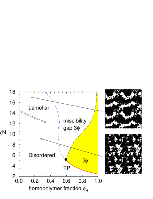
Abbildung 1: Phase diagram for a ternary symmetrical A+B+AB blend from Monte Carlo simulations of the bond fluctuation model as a function of the incompatibility parameter $\chi N$ and the homopolymer volume fraction $\Phi_{C}$. The chain length of all three species is equal, $N=32$ corresponding to ${\bar{\cal N}}=91$. 2$\phi$ denotes a region of two-phase coexistence between an A-rich and a B-rich phase, 3 $\phi$ one of three-phase coexistence between an A-rich, a B-rich, and a lamellar phase. Slice through the three-dimensional system of linear dimension $L=4.7R_{e}$ and three periodic images are shown on the left hand side. From Ref. MMCOP .

Capillary waves do not only broaden the width of the interface, but they can also destroy the orientational order in highly swollen lamellar phases. Those phases occur in mixtures of diblock-copolymers and homopolymers. The addition of homopolymers swells the distance between the lamellae, and the self-consistent field theory predicts that this distance diverges at Lifshitz points. However, general considerations show that mean-field approximations are bound to break down in the vicinity of Lifshitz points HOLYST . (The upper critical dimension is $d_{u}=8$). This can be quantified by a Ginzburg criterion. Fluctuations are important if

$$t\equiv\frac{\chi N-\chi_{t}N}{\chi_{t}N}\ll{\bar{\cal N}}^{-2/5}$$ (73)

The Ginzburg criterion has a simple heuristic interpretation: Fluctuations of the interface position destroy the long-ranged lamellar order. Those interface fluctuations are not limited by the increase of the surface area ($\gamma=0$), but rather by the bending stiffness $\kappa$. The correlation length $\xi_{n}$ of the direction of a single, stiff interface is given by $\xi_{n}\sim\exp(2\pi\kappa/k_{B}T)$ TAUPIN . If the stiffness $\kappa$ is of order unity, there is no long-range order of the normal direction of the interface, and the lamellar order will be replaced by a microemulsion-like structure. In the vicinity of a Lifshitz point self-consistent field theory predicts the interface stiffness to vanish like $\kappa\sim k_{B}T\sqrt{{\bar{\cal N}}}t^{5/4}$ which is compatible with the Ginzburg criterion (73) GERHARD .

Similar arguments hold for a tricritical Lifshitz point, where a Lifshitz point happens to merge with a regular tricritical point. Here, fluctuations are important if

$$t\equiv\frac{\chi N-\chi_{t}N}{\chi_{t}N}\ll{\bar{\cal N}}^{-2/3}$$ (74)

Again this behavior is compatible with the behavior of the bending stiffness, $\kappa\sim k_{B}T\sqrt{{\bar{\cal N}}}t^{3/4}$, as obtained from self-consistent field calculations GERHARD .

5) Phase diagram of random copolymers

Macrophase separation can also occur in random copolymers FML , which consist of a random sequence of $Q$ blocks, each of which comprises either $M$ segments of type $A$ or $M$ segments of type $B$. Macrophase separation occurs when $\chi M$ is of order unity, i. e., independent from the number of blocks, and the $A$-rich and $B$-rich phases differ in their composition only by an amount of order $1/\sqrt{Q}$. The strength of fluctuation effects can be quantified by the Ginzburg number JEROME

$${\rm Gi}\sim\frac{Q^{2}}{\bar{\cal M}}\qquad\mbox{with}\qquad\bar{\cal M}=\left(\rho_{m}R^{3}_{M}/M\right)^{2}$$ (75)

where $\rho_{m}=N{\varrho}$ denotes the monomer number density. While Gi decreases in the case of homopolymer mixtures like $1/{\bar{\cal N}}$, it increases quadratically in the number of blocks for random copolymers. In other words, if we increase the number of blocks per molecule, fluctuation effects become stronger and stronger. Indeed, Monte Carlo simulations indicate the presence of a disordered, microemulsion-like structure in much of the parameter region where mean-field theory predicts macrophase separation.

In all but the last example, fluctuation effects in three dimensions are controlled by the chain length $N$, in the sense that if $N\sim{\bar{\cal N}}\to\infty$, fluctuations effects can be made arbitrary small. This provides a formal limit in which self-consistent field theory becomes accurate. We emphasize, however, that in many practical examples fluctuations are very important. For instance, the broadening of the interface width by capillary waves is typically a sizeable fraction of the intrinsic width calculated by self-consistent field theory.

In particle-based models, the mean-field approximation also neglects short-ranged correlations in the polymeric fluid, e. g., the fluid-like packing of the particles or the correlations due to the self-avoidance of the polymers on short length scales. There is no small parameter which controls the magnitude of these correlation effects, but they are incorporated into the coarse-grained parameters $R_{e}$ and $\chi N$.

4.2 Gaussian fluctuations and Random Phase Approximation

As long as fluctuations are weak, they can be treated within the Gaussian approximation. One famous example of such a treatment is the random phase approximation (RPA), which describes Gaussian fluctuations in homogeneous phases. The RPA has been extended to inhomogeneous saddle points by Shi, Noolandi, and coworkers shi ; laradji . In this section, we shall re-derive this generalized RPA theory within the formalism developed in the previous sections.

Our starting point is the Hamiltonian ${\cal G}[U,W]$ of Eq. (11). We begin with expanding it up to second order about the saddle point $\bar{{\cal G}}={\cal G}[U^{*},W^{*}]$ of the SCF theory. To this end, we define the averaged single chain correlation functions review ; shi ; laradji

$$K_{\alpha\beta}({\bf r},{\bf r}^{\prime})=-\frac{\delta\phi_{\alpha}^{*}}{\delta W_{\beta}}=\frac{1}{{\varrho}}\sum_{J}n_{J}\frac{\delta^{2}\ln{\cal V}Q_{J}[W_{A},W_{B}]}{\delta W_{\alpha}({\bf r})\>\delta W_{\beta}({\bf r}^{\prime})}$$ (76)

with $\alpha,\beta=A$ or $B$, where $\phi_{\alpha}^{*}$ is defined as in Eq. (2.2), and all derivatives are evaluated at the saddle point values of the fields, $W_{A}^{*}=(iU^{*}+W^{*})/2$ and $W_{B}^{*}=(iU^{*}-W^{*})/2)$. As usual the sum $J$ runs over the different types of polymers in the mixture, and $n_{J}$ denotes the total number of polymers of type $J$. In the case of a homopolymer mixture, the mixed correlation functions $K_{AB}({\bf r},{\bf r}^{\prime})$, $K_{BA}({\bf r},{\bf r}^{\prime})$ are zero.

With these definitions, the quadratic expansion of ${\cal G}[U,W]$ (11) can be written as

$$\frac{{\cal G}[U,W]-\bar{\cal G}}{\sqrt{{\bar{\cal N}}}k_{B}T({\cal V}/{R_{e}^{d}})} = \frac{1}{{\cal V}}\>\frac{1}{4\chi N}\int{{\rm d}^{d}{\bf r}}\>\delta W({\bf r})^{2}$$ (77)

$$-\>\frac{1}{2{\cal V}}\sum_{\alpha\beta}\int{{\rm d}^{d}{\bf r}}\>d^{3}{\bf r}^{\prime}K_{\alpha\beta}({\bf r},{\bf r}^{\prime})\>\delta W_{\alpha}({\bf r})\>\delta W_{\beta}({\bf r}^{\prime})$$

$$\mbox{with}\qquad\delta W_{A}=(i\delta U+\delta W)/2,\qquad\delta W_{B}=(i\delta U-\delta W)/2.$$

Since $\bar{\cal G}$ is an extremum, the linear terms in $\delta U$ and $\delta W$ vanish. Next we expand this expression in $\delta U$ and $\delta W$. To simplify the expressions, we follow Laradji et al., define review ; laradji

$$\Sigma = K_{AA}+K_{AB}+K_{BA}+K_{BB}$$ (78)

$$C = K_{AA}-K_{AB}-K_{BA}+K_{BB}$$ (79)

$$\Delta = K_{AA}+K_{AB}-K_{BA}-K_{BB}$$ (80)

$$\Delta^{+} = K_{AA}-K_{AB}+K_{BA}-K_{BB},$$ (81)

and adopt the matrix notation

$$\delta A\cdot K\cdot\delta B\equiv\int{{\rm d}^{d}{\bf r}}\>{\rm d}^{d}{\bf r}^{\prime}K({\bf r},{\bf r}^{\prime})\>\delta A({\bf r})\>\delta B({\bf r}^{\prime}).$$

with the unity operator ${\bf 1}=\delta({\bf r}-{\bf r}^{\prime})$. Note that the operators $\Sigma$ and $C$ are symmetric, and $\Delta$ and $\Delta^{+}$ are transposed to each other. In the new notation, Eq. (77) reads

$$\frac{{\cal G}[U,W]-\bar{\cal G}}{\sqrt{{\bar{\cal N}}}k_{B}T({\cal V}/{R_{e}^{d}})}=\frac{1}{{\cal V}}\>\frac{1}{4\chi N}\delta W\cdot{\bf 1}\cdot\delta W$$

$$+\>\frac{1}{8{\cal V}}\left(\delta U\cdot\Sigma\cdot\delta U-\delta W\cdot C\cdot\delta W+i\delta W\cdot\Delta\cdot\delta U+i\delta U\cdot\Delta^{+}\cdot\delta W\right).$$

and can, after some algebra, be cast in the form

$$\frac{{\cal G}[U,W]-\bar{\cal G}}{\sqrt{{\bar{\cal N}}}k_{B}T({\cal V}/{R_{e}^{d}})}=$$

$$\frac{1}{8{\cal V}}\left\{(\delta U-\delta U^{*})\cdot\Sigma\cdot(\delta U-\delta U^{*})+\frac{2}{\chi N}\delta W\cdot[{\bf 1}-\frac{\chi N}{2}\tilde{C}]\cdot\delta W\right\}$$

$$\mbox{with}\quad\tilde{C}=C-\Delta\cdot\Sigma^{-1}\cdot\Delta^{+}\qquad\mbox{and}\qquad\delta U^{*}=-i\Sigma^{-1}\cdot\Delta^{+}\cdot\delta W.$$ (84)

The field $U^{*}+\delta U^{*}$ corresponds to the saddle point of ${\cal G}[U,W]$ at fixed $W=W^{*}+\delta W$.

Both the fluctuations $\langle\delta W^{2}\rangle$ and $\langle(\delta U-\delta U^{*})\rangle$ decrease like $1/\sqrt{{\bar{\cal N}}}$. However, the fluctuations in both fields are qualitatively different. The operator $\Sigma$ is positive, i. e., the eigenvalues of $\Sigma$ are positive, therefore fluctuations in $U$ remain small and the Gaussian approximation is justified in the limit of large $\sqrt{{\bar{\cal N}}}$. The operator ${\bf 1}-\chi N/2\tilde{C}$, on the other hand, may have negative eigenvalues at large $\chi$. In that case the saddle point under consideration is unstable and the true solution of the SCF theory corresponds to a different structure (phase). A saddle point which turns from being stable to unstable defines a spinodal or a continuous phase transition. In addition, the operator ${\bf 1}-\chi N/2\tilde{C}$ also has zero eigenvalues in the presence of continuous symmetries. In all of these cases, the expansion for small $\delta W$ becomes inaccurate and fluctuations in $\delta W$ may give rise to qualitative deviations from the mean-field theory.

Within the Gaussian approximation, the average $\langle W({\bf r})W({\bf r}^{\prime})\rangle$ can readily be calculated:

$$\langle W({\bf r})W({\bf r}^{\prime})\rangle=W^{*}({\bf r})W^{*}({\bf r}^{\prime})+\frac{2\chi N}{\sqrt{{\bar{\cal N}}}}{R_{e}^{d}}\>\Big{[}{\bf 1}-\frac{\chi N}{2}\tilde{C}\Big{]}^{-1}_{{\bf r},{\bf r}^{\prime}}$$ (85)

Using the relation between fluctuations of $W$ and the composition, Eq. (2.2), we obtain

$$\langle[\hat{\phi}_{A}({\bf r})-\hat{\phi}_{B}({\bf r})][\hat{\phi}_{A}({\bf r^{\prime}})-\hat{\phi}_{B}({\bf r^{\prime}})]\rangle-\langle\hat{\phi}_{A}({\bf r})-\hat{\phi}_{B}({\bf r})\rangle\langle\hat{\phi}_{A}({\bf r}^{\prime})-\hat{\phi}_{B}({\bf r}^{\prime})\rangle$$ (86)

$$\equiv \frac{2{R_{e}^{d}}}{\sqrt{{\bar{\cal N}}}\chi N}\left[\Big{[}{\bf 1}-\frac{\chi N}{2}\tilde{C}\Big{]}^{-1}-{\bf 1}\right]_{{\bf r},{\bf r}^{\prime}}$$

$$= \frac{2{R_{e}^{d}}}{\sqrt{{\bar{\cal N}}}\chi N}\left[\sum_{k=1}^{\infty}\Big{[}\frac{\chi N}{2}\tilde{C}\Big{]}^{k}\right]_{{\bf r},{\bf r}^{\prime}}=\frac{1}{\sqrt{{\bar{\cal N}}}}\left[\tilde{C}\Big{[}{\bf 1}-\frac{\chi N}{2}\tilde{C}\Big{]}\right]_{{\bf r},{\bf r}^{\prime}}^{-1}$$

$$= \frac{1}{\sqrt{{\bar{\cal N}}}}\Big{[}\tilde{C}^{-1}-\frac{\chi N}{2}{\bf 1}\Big{]}^{-1}_{{\bf r},{\bf r}^{\prime}}.$$

This is the general expression for Gaussian composition fluctuations in incompressible polymer blends derived from EP theory. The original derivation of Shi, Noolandi and coworkers shi ; laradji uses as a starting point the density functional (53) and gives the identical result. A generalization for compressible blends can be found in Ref. review .

The special situation of a homogeneous saddle point, corresponding to a homogeneous disordered phase, is particularly interesting. In that case, explicit analytical relations between the single chain partition function and the fields can be obtained, and one recovers the well-known random phase approximation (RPA). To illustrate this approach, we shall now derive the RPA structure factor for the case of a symmetrical binary homopolymer blend.

Since the reference saddle point is spatially homogeneous, all correlation functions $K_{\alpha\beta}({\bf r},{\bf r}^{\prime})$ only depend on (${\bf r}-{\bf r}^{\prime}$) and it is convenient to perform the calculations in Fourier space. We use the following conventions for the Fourier expansion:

$$\hat{\phi}({\mathbf{r}})=\bar{\phi}+\sum_{{\mathbf{q}}\neq 0}\phi_{\mathbf{q}}e^{i\mathbf{qr}}\qquad\qquad\phi_{\mathbf{q}}=\frac{1}{{\cal V}}\int{{\rm d}^{d}{\bf r}}\;\hat{\phi}({\mathbf{r}})e^{-i\mathbf{qr}}.$$ (87)

In homopolymer melts, the mixed single chain correlation functions $K_{AB}$, $K_{BA}$ vanish, thus one has $C=\Sigma=K_{AA}+K_{BB}$ and $\Delta=\Delta^{+}=K_{AA}-K_{BB}$. An explicit expression for the functional $\phi_{A}^{*}({\bf r})=\bar{\phi}_{A}\langle\hat{\phi}_{A}({\bf r})\rangle$ in the limit of small fields $W_{A}$ can be derived:

$$\phi_{A}^{*}({\bf r}) = \bar{\phi}_{A}\left(1-\sum_{{\bf q}\neq 0}g_{A}({\bf q})W_{A{\bf q}}e^{i\mathbf{qr}}\right)$$ (88)

$$= \bar{\phi}_{A}\left(1-\frac{1}{{\cal V}}\int{{\rm d}^{d}{\bf r}}^{\prime}\sum_{{\bf q}\neq 0}g_{A}({\bf q})W_{A}({\bf r}^{\prime})e^{i{\bf q}({\bf r}-{\bf r}^{\prime})}\right)$$

A similar expressions holds for $\phi_{B}^{*}({\bf r})$. Here $g({\bf q})=(2/x^{2})(\exp[-x]-1+x)$ with $x\equiv R_{e}^{2}{\bf q}^{2}/6$ denotes the Debye function. Hence, the Fourier transform of $K_{AA}$ can be identified with the single chain structure factor:

$$K_{AA}({\bf r},{\bf r}^{\prime}) = -\frac{\delta\phi_{A}^{*}({\bf r})}{\delta W_{A}({\bf r}^{\prime})}=\bar{\phi}_{A}\frac{1}{{\cal V}}\sum_{{\bf q}\neq 0}g_{A}({\bf q})e^{i{\bf q}({\bf r}-{\bf r}^{\prime})}$$

$$K_{AA}({\bf q}) = \bar{\phi}_{A}g_{A}({\bf q}),$$ (89)

and a similar expression holds $K_{BB}$. Using the definition of $\tilde{C}$, Eq. (84), one obtains

$$\tilde{C}^{-1}=\frac{1}{4}\Big{[}\frac{1}{K_{AA}}+\frac{1}{K_{BB}}\Big{]}=\frac{1}{4}\Big{[}\frac{1}{\bar{\phi}_{A}g_{A}}+\frac{1}{\bar{\phi}_{B}g_{B}}\Big{]}.$$

Inserting this expression into Eq. (86), we can also obtain an explicit expression for the EP Hamiltonian ${\cal H}[W]\equiv{\cal G}[U^{*},W]$ of binary blends within RPA:

$$\frac{{\cal H}_{\rm RPA}[W]-\bar{\cal H}}{\sqrt{{\bar{\cal N}}}k_{B}T({\cal V}/{R_{e}^{d}})} = +\frac{1}{8}\sum_{{\mathbf{q}}\neq 0}\left(\frac{2}{\chi N}-\frac{4\bar{\phi}_{A}g_{A}({\mathbf{q}})\bar{\phi}_{B}g_{B}({\mathbf{q}})}{\bar{\phi}_{A}g_{A}({\mathbf{q}})+\bar{\phi}_{B}g_{B}({\mathbf{q}})}\right)|W_{\mathbf{q}}|^{2}$$ (90)

Combined with Eq. (2.2), this yields the well-known RPA expression for the collective structure factor in binary polymer blends

$$\frac{4}{\sqrt{{\bar{\cal N}}}({\cal V}/{R_{e}^{d}})\langle|\phi_{A{\bf q}}-\phi_{B{\bf q}}|^{2}\rangle}=\frac{1}{\bar{\phi}_{A}g_{A}({\bf q})}+\frac{1}{\bar{\phi}_{B}g_{B}({\bf q})}-2\chi N.$$ (91)

This calculation also justifies the use of Eq. (2.2) to calculate the fluctuations in the EP theory ELLEN1 . If we used the literal fluctuations in the EP theory according of Eq. (2), we would not recover the RPA expression but rather ELLEN1

$$\langle|\hat{\phi}_{{A\mathbf{q}}}-\hat{\phi}_{B{\bf q}}|^{2}\rangle_{\rm EP}$$ (92)

$$= \langle|\phi^{*}_{{A\mathbf{q}}}-\phi^{*}_{B{\bf q}}|^{2}\rangle-\frac{{R_{e}^{d}}}{\sqrt{\bar{N}}V^{2}}\int{{\rm d}^{d}{\bf r}}\;{\rm d}^{3}{\bf r}^{\prime}\;e^{i{\bf q}({\bf r}-{\bf r}^{\prime})}\left\langle\frac{\delta\phi^{*}_{A}({\bf r})}{\delta W_{A}({\bf r}^{\prime})}+\frac{\delta\phi^{*}_{B}({\bf r})}{\delta W_{B}({\bf r}^{\prime})}\right\rangle$$

$$= \frac{8\chi Ng^{2}({\bf q})\bar{\phi}_{A}^{2}\bar{\phi}_{B}^{2}}{\sqrt{{\bar{\cal N}}}(V/{R_{e}^{d}})(1-2\chi N\bar{\phi}_{A}\bar{\phi}_{B}g({\bf q}))}+\frac{g({\bf q})}{\sqrt{{\bar{\cal N}}}(V/{R_{e}^{d}})}$$

$$= \langle|\hat{\phi}_{{A\mathbf{q}}}-\hat{\phi}_{B{\bf q}}|^{2}\rangle+\frac{(1-4\bar{\phi}_{A}\bar{\phi}_{B})g({\bf q})}{\sqrt{{\bar{\cal N}}}(V/{R_{e}^{d}})}.$$

Both contributions are of the same order.

This example illustrates how the RPA can be used to derive explicit, analytical expressions for Hamiltonians structure factors. The generalization to blends that also contain copolymers is straightforward.

4.3 Relation to Ginzburg-Landau models

In order to make the connection to a Landau-Ginzburg theory for binary blends, we study the behavior of the structure factor at small wavevectors $q$ for a symmetric mixture. Using $g(q)\approx 1+\frac{(qR_{e})^{2}}{18}+\cdots$ we obtain:

$$\frac{4}{\sqrt{{\bar{\cal N}}}(V/{R_{e}^{d}})\langle|\phi_{A{\bf q}}-\phi_{B{\bf q}}|^{2}\rangle}=\frac{1}{\bar{\phi}_{A}}+\frac{1}{\bar{\phi}_{B}}-2\chi N+\frac{q^{2}R_{e}^{2}}{18\bar{\phi}_{A}}+\frac{q^{2}R_{e}^{2}}{18\bar{\phi}_{B}}$$ (93)

If we assume composition fluctuations to be Gaussian, we can write down a free energy functional compatible with equation (91).

$$\frac{{\cal F}_{\rm RPA}[\phi_{A{\bf q}}]}{\sqrt{{\bar{\cal N}}}k_{B}T(V/{R_{e}^{d}})}=\frac{1}{\sqrt{{\bar{\cal N}}}(V/{R_{e}^{d}})}\frac{(2\phi_{A{\bf q}}-1)^{2}}{2\langle|\phi_{A{\bf q}}-\phi_{B{\bf q}}|^{2}\rangle}$$

$$= \frac{1}{2}\left(\frac{1}{\bar{\phi}_{A}}+\frac{1}{1-\bar{\phi}_{A}}-2\chi N\right)|\phi_{A{0}}-\bar{\phi}_{A}|^{2}$$

$$+\frac{1}{2}\sum_{{\bf q}\neq 0}\left(\frac{1}{\bar{\phi}_{A}}+\frac{1}{1-\bar{\phi}_{A}}-2\chi N+\frac{q^{2}R_{e}^{2}}{18\bar{\phi}_{A}}+\frac{q^{2}R_{e}^{2}}{18(1-\bar{\phi}_{A})}\right)|\phi_{A{\bf q}}|^{2}$$

Note that this free energy functional is Gaussian in the Fourier coefficients of the composition, and, hence, the critical behavior still is of mean-field type. Transforming back from Fourier expansion for the spatial dependence to real space, we obtain for the free energy functional:

$$\frac{{\cal F}_{\rm RPA}[\phi_{A}({\bf r})]}{\sqrt{{\bar{\cal N}}}k_{B}T({\cal V}/{R_{e}^{d}})} = \frac{1}{{\cal V}}\int{{\rm d}^{d}{\bf r}}\;\left\{\frac{1}{2}\left(\frac{1}{\bar{\phi}_{A}}+\frac{1}{1-\bar{\phi}_{A}}-2\chi N\right)\left(\phi_{A}({\bf r})-\frac{1}{2}\right)^{2}\right.$$

$$\hskip 42.67912pt\left.+\frac{R_{e}^{2}}{36\bar{\phi}_{A}(1-\bar{\phi}_{A})}(\nabla\phi_{A})^{2}\right\}$$

$$= \frac{1}{{\cal V}}\int{{\rm d}^{d}{\bf r}}\;\left\{\frac{1}{2}\frac{{\rm d}^{2}f_{\rm FH}}{{\rm d}\bar{\phi}_{A}^{2}}\left(\phi_{A}({\bf r})-\frac{1}{2}\right)^{2}+\frac{R_{e}^{2}(\nabla\phi_{A})^{2}}{36\bar{\phi}_{A}(1-\bar{\phi}_{A})}\right\}$$

Expanding the free energy of the homogeneous system (Flory-Huggins free energy of mixing), we can restore higher order terms and obtain the Landau-de Gennes free energy functional for a symmetric binary polymer blend:

$$\frac{{\cal F}_{\rm GL}[\phi_{A}({\bf r})]}{\sqrt{{\bar{\cal N}}}k_{B}T({\cal V}/{R_{e}^{d}})} = \frac{1}{{\cal V}}\int{{\rm d}^{d}{\bf r}}\;\left\{f_{\rm FH}(\phi_{A})+\frac{R_{e}^{2}}{36\bar{\phi}_{A}(1-\bar{\phi}_{A})}(\nabla\phi_{A})^{2}\right\}$$ (96)

$$= \frac{1}{{\cal V}}\int{{\rm d}^{d}{\bf r}}\;\left\{(2-\chi N)\left(\phi_{A}({\bf r})-\frac{1}{2}\right)^{2}+\frac{4}{3}\left(\phi_{A}({\bf r})-\frac{1}{2}\right)^{4}\right.$$

$$\hskip 42.67912pt\left.+\frac{R_{e}^{2}}{36\bar{\phi}_{A}(1-\bar{\phi}_{A})}(\nabla\phi_{A})^{2}\right\}$$

A field-theory based on this simple expansion will already yield the correct three-dimensional Ising critical behavior. Note that the non-trivial critical behavior is related to higher order terms in $W$ or $\phi_{A}-\phi_{B}$. Fluctuations in the incompressibility field $U$ or the total density $\phi_{A}+\phi_{B}$ are not important.

4.4 Field-theoretic polymer simulations

Studying fluctuations beyond the Gaussian approximation is difficult. Special types of fluctuations, e. g., capillary wave fluctuations of interfaces, can sometimes be described analytically within suitable approximations andreas . The only truly general methods are however computer simulations. Here we shall discuss two different approaches to simulating field theories for polymers: Langevin simulations and Monte Carlo simulations.

4.4.1 Langevin simulations

As long as one is mainly interested in composition fluctuations (EP approximation, see section 3), the problem can be treated by simulation of a real Langevin process. The correct ensemble is reproduced by the dynamical equation

$$\frac{\partial W({\bf r},t)}{\partial t}=-\int{\rm d}^{d}{\bf r}^{\prime}M({\bf r},{\bf r}^{\prime})\frac{\delta{\cal H}[W]}{\delta W({\bf r}^{\prime},t)}+\theta({\bf r},t),$$ (97)

where $M({\bf r},{\bf r}^{\prime})$ is an (arbitrary) kinetic coefficient, and $\theta({\bf r},t)$ is a stochastic noise. The first two moments of $\theta$ are fixed by the fluctuation-dissipation theorem

$$\langle\theta\rangle=0\qquad\langle\theta({\bf r},t)\theta({\bf r}^{\prime},t)\rangle=2k_{B}TM({\bf r},{\bf r}^{\prime})\>\delta({\bf r}-{\bf r}^{\prime})\>\delta(t-t^{\prime}).$$ (98)

The choice of $M({\bf r},{\bf r}^{\prime})$ determines the dynamical properties of the system. For example, $M({\bf r},{\bf r}^{\prime})=\delta({\bf r}-{\bf r}^{\prime})/\tau k_{B}T$ corresponds to a non-conserved field, while field conservation can be enforced by using a kinetic coefficient of the form $M({\bf r},{\bf r}^{\prime})=\nabla_{{\bf r}}\Lambda({\bf r}-{\bf r}^{\prime})\nabla_{{\bf r}^{\prime}}$. Different forms for the Onsager coefficient $\Lambda$ will be discussed in Sec. 5. In each step of the Langevin simulation one updates all field variables simultaneously ELLEN1 and the the self-consistent equations for the saddle point $U^{*}(W)$ have to be solved.

The approach is commonly referred to as external potential dynamics (EPD). A related approach has originally been introduced by Maurits and Fraaije maurits . However, these authors do not determine $U^{*}(W)$ exactly, but only approximately by solving separate Langevin equations for real fields $W_{A}$ and $W_{B}$. This amounts to introducing a separate Langevin equation for a real field $iU$ (i. e., an imaginary $U$ in our notation) in addition to Eq. (97).

As the fluctuation effects discussed earlier (cf. Sec. 4.1) are essentially caused by composition fluctuations, the EP approximation seems reasonable. Nevertheless, one would also like to study the full fluctuating field theory by computer simulations. In attempting to do so, however, one faces a serious problem: Since the field $iU$ is imaginary, the Hamiltonian ${\cal G}$ is in general complex, and the “weight” factor $\exp[-{\cal G}]$ can no longer be used to generate a probability function. This is an example of a sign problem, as is well-known from other areas of physics signproblem , e. g., lattice gauge theories and correlated fermion theories. A number of methods have been devised to handle complex Hamiltonians or complex actions klauder ; parisi ; lin ; baeurle ; andre . Unfortunately, none of them is as universally powerful as the methods that sample real actions (Langevin simulations, Monte Carlo, etc. ).

Fredrickson and coworkers venkat ; glenn_review ; glenn2 ; alexander have recently introduced the complex Langevin method klauder ; parisi into the field of polymer science. The idea of this method is simply to extend the real Langevin formalism, e. g., as used in EPD, to the case of a complex action. The drift term $\delta{\cal H}/\delta W$ in Eq. 97 is replaced by complex drift terms $\delta{\cal G}[U,W]/\delta U$ and $\delta{\cal G}[U,W]/\delta W$, which govern the dynamics of complex fields $U$ and $W$. This generates a diffusion process in the entire complex plane for both $U$ and $W$. One might wonder why such a process should sample line integrals over $U$ and $W$. To understand that, one must recall that the integration paths of the line integrals can be distorted arbitrarily in the complex plane, as long as no pole is crossed, without changing the result. Hence a complex Langevin trajectory samples an ensemble of possible line integrals. Under certain conditions, the density distribution converges towards a stationary distribution which indeed reproduces the desired expectation values gausterer . Unfortunately, these conditions are not generally satisfied, and cases have been reported where a complex Langevin process did not converge at all, or converged towards the wrong distribution lin ; schoenmakers . Thus the theoretical foundations of this methods are still under debate. In the context of polymer simulations, however, no problems with the convergence or the uniqueness of the solution were reported.

In our case, the complex Langevin equations that simulate the Hamiltonian (11) read

$$\frac{\partial U({\bf r},t)}{\partial t} = -\frac{\delta{\cal G}[U,W]/k_{B}T}{\delta U({\bf r},t)}+\>\theta_{U}({\bf r},t)$$ (99)

$$\frac{\partial W({\bf r},t)}{\partial t} = -\frac{\delta{\cal G}[U,W]/k_{B}T}{\delta W({\bf r},t)}+\theta_{W}({\bf r},t),$$ (100)

where $\theta_{U}({\bf r},t)$, $\theta_{W}({\bf r},t)$ are real Gaussian white noises which satisfy the fluctuation-dissipation theorem

$$\langle\theta\rangle=0\qquad\langle\theta({\bf r},t)\theta({\bf r}^{\prime},t)\rangle=2\>\delta({\bf r}-{\bf r}^{\prime})\>\delta(t-t^{\prime}).$$ (101)

The partial derivatives are given by

$$\frac{\delta{\cal G}[U,W]/k_{B}T}{\delta W({\bf r},t)} = \frac{\sqrt{{\bar{\cal N}}}}{2{R_{e}^{d}}}\>\Big{[}\frac{W}{\chi N}+\phi_{A}^{*}-\phi_{B}^{*}\Big{]}$$ (102)

$$\frac{\delta{\cal G}[U,W]/k_{B}T}{\delta U({\bf r},t)} = \frac{\sqrt{{\bar{\cal N}}}}{2{R_{e}^{d}}}\>\Big{[}\phi_{A}^{*}+\phi_{B}^{*}-1\Big{]},$$ (103)

with $\phi_{A}^{*}$ and $\phi_{B}^{*}$ defined as in Eq. (2.2).

If the noise term is turned off, the system is driven towards the nearest saddle point. Therefore, the same set of equations can be used to find and test mean-field solutions. The complex Langevin method was first applied to dense melts of copolymers venkat , and later to mixtures of homopolymers and copolymers dominik1 and to diluted polymers confined in a slit under good solvent conditions alexander . Fig. 2 shows examples of average “density” configurations $\langle\phi^{*}\rangle$ for a ternary block copolymer/ homopolymer system above and below the order/disorder transition.

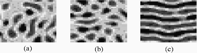
Abbildung 2: Averaged densities across the order-disorder transition in a two-dimensional ternary system with A,B homopolymers and A-B copolymers (20 % homopolymer volume fraction), as obtained from Complex Langevin simulation runs.

4.4.2 Field-theoretic Monte Carlo

As an alternative approach to sampling the fluctuating field theory, Düchs et al. dominik_diss ; dominik1 have proposed a Monte Carlo method. Since the weight $\exp[-{\cal G}]$ is not positive semidefinite, the Monte Carlo algorithm cannot be applied directly. To avoid this problem, we split ${\cal G}$ into a real and an imaginary part ${\cal G}^{R}$ and $i{\cal G}^{I}$ and sample only the real contribution $\exp(-{\cal G}^{R})$ lin . The imaginary contribution is incorporated into a complex reweighting factor $\exp(-i{\cal G}^{I})$. Statistical averages over configurations $j$ then have to be computed according to

$$\langle A\rangle=\frac{\sum_{j}\exp(-i{\cal G}^{I}_{j})A_{j}}{\sum_{j}\exp(-i{\cal G}^{I}_{j})},$$ (104)

i. e., every configuration is weighted with this factor. Furthermore, we premise that the (real) saddle point $iU^{*}$ contributes substantially to the integral over the imaginary field $iU$ and shift the integration path such that it passes through the saddle point. The field $iU$ is then represented as

$$iU=iU^{*}[W]+i\omega,$$ (105)

where $\omega$ is real.

The Monte Carlo simulation includes two different types of moves: trial moves of $W$ and $\omega$. The moves in $\omega$ are straightforward. Implementing the moves in $W$ is more involved. Every time that $W$ is changed, the new saddle point $iU^{*}[W]$ must be evaluated. In an incompressible blend, the set of self consistent equations

$$\phi_{A}^{*}({\bf r})+\phi_{B}^{*}({\bf r})=1,\qquad\forall{\bf r}$$ (106)

must be solved for $iU^{*}$. Fortunately, this does not require too many iterations, if $W$ does not vary very much from one Monte Carlo step to another.

Compared to the Complex Langevin method, the Monte Carlo method has the advantage of being well founded theoretically. However, it can become very inefficient when ${\cal G}^{I}$ spreads over a wide range and the reweighting factor oscillates strongly. In practice, it relies on the fact that the integral is indeed dominated by one (or several) saddle points.

Can we expect this to be the case here? To estimate the range of the reweighting factor, we briefly re-inspect the Hubbard-Stratonovich transformation of the total density $\hat{\phi}_{A}+\hat{\phi}_{B}$ that lead to the fluctuating field $U$. For simplicity we consider a one-component system. In a compressible polymer solution or blend, the contribution of the repulsive interaction energy to the partition function can be written as

$$\exp\Big{[}-{\varrho}N\frac{\kappa}{2}\int{{\rm d}^{d}{\bf r}}(\hat{\phi}_{A}+\hat{\phi}_{B}-\phi_{0})^{2}\Big{]}$$ (107)

(with $\phi_{0}=1$ in a melt, and $\phi_{0}=0$ in a good solvent). The Hubbard-Stratonovich transformation of this expression is proportional to

$$\int{\cal D}U\exp\Big{[}-{\varrho}\Big{\{}\frac{1}{8\kappa N}\int{{\rm d}^{d}{\bf r}}\;U^{2}+i\int{{\rm d}^{d}{\bf r}}\;\frac{U}{2}(\hat{\phi}_{A}+\hat{\phi}_{B}-\phi_{0})\Big{\}}\Big{]}$$ (108)

Thus $U$ should to be distributed around the saddle point with a width proportional to $\kappa$. The method should work best for very compressible solutions with small $\kappa$. In contrast, in a compressible blend, the contribution (107) is replaced by a delta function constraint $\delta(\hat{\phi}_{A}+\hat{\phi}_{B}-1)$. The fluctuating field representation of this constraint is

$$\int{\cal D}U\exp[-i{\varrho}\int{{\rm d}^{d}{\bf r}}\;\frac{U}{2}(\hat{\phi}_{A}+\hat{\phi}_{B}-1)].$$ (109)

The only forces driving $U$ towards the saddle point are now those related to the single chain fluctuations (cf. Sec. 4.2), and $U$ will be widely distributed on the imaginary axis. Thus it is not clear whether the Monte Carlo method will work for incompressible systems.

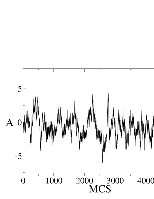
Abbildung 3: Argument ${\cal G}^{I}$ of the reweighting factor in a simulation of an incompressible blend. From Ref. dominik1 .

Indeed, simulations of an incompressible ternary A+B+AB homopolymer / copolymer blend showed that the values of the argument ${\cal G}^{I}$ of the reweighting factor cover a wide range (Fig. 3). Hence computing statistical averages becomes very difficult, because both the numerator and the denominator in Eq. (104) are subject to very large relative errors.

Fortunately, a closer inspection of the data reveals that the reweighting factor is entirely uncorrelated with the fluctuating field $W$. Since the latter determines all quantities of interest to us (Eq. (25) and (2.2)), the averages can be computed without reweighting. Moreover, the time scales for variations of $W$ and $\omega$ are decoupled. By sampling $\omega$ more often than $W$, they can be chosen such that the time scale of $\omega$ is much shorter than that of $W$. Finally, the dynamics of the actual simulation, which is governed by the real factor $\exp(-{\cal G}^{R})$, is virtually the same as that of a reference simulation with $\omega$ switched off dominik1 .

Combining all these observations, we infer that the fluctuations in $\omega$ do not influence the composition structure of the blend substantially. A similar decoupling between composition and density fluctuations is suggested by other studies PRISM ; VILGIS ; MREV . The composition structure can equivalently be studied in a Monte Carlo simulation which samples only $W$ and sets $\omega\equiv 0$. We have demonstrated this for one specific case of an incompressible blend and suspect that it may be a feature of incompressible blends in general. The observation that the fluctuations in $W$ and $\omega$ are not correlated with each other is presumably related to the fact that the (vanishing) density fluctuations do not influence the composition fluctuations. If that is true, we can conclude that field-theoretic Monte Carlo can be used to study fluctuations in polymer mixtures in the limits of high and low compressibilities. Whether it can also be applied at intermediate compressibilities will have to be explored in the future.

Fig. 4 shows examples of snapshots for the ternary system in the vicinity of the order-disorder transition.

Abbildung 4: Snapshots of $\phi_{A}^{*}$ for the same ternary A+B+AB system as in Fig. 2, at 70 % homopolymer volume fraction, for different $\chi N$ above and below the order-disorder transition, as obtained from Monte Carlo simulations with $\omega$ switched off (EP theory). From Ref. dominik2 .

We should note that the Monte-Carlo simulation with $\omega\equiv 0$ effectively samples the EP Hamiltonian. This version of field-theoretic Monte Carlo is equivalent to the real Langevin method (EPD), and can be used as an alternative. Monte Carlo methods are more versatile than Langevin methods, because an almost unlimited number of moves can be invented and implemented. In our applications, the $W$ and $\omega$-moves simply consisted of random increments of the local field values, within ranges that were chosen such that the Metropolis acceptance rate was roughly 35%. On principle, much more sophisticated moves are conceivable, e. g., collective moves or combined EPD/Monte Carlo moves (hybrid moves HYBRID ). On the other hand, EPD is clearly superior to Monte Carlo when dynamical properties are studied. This will be discussed in the next section.

5 Dynamics

5.1 Onsager coefficients and dynamic SCF theory (DSCFT)

In order to describe the diffusive dynamics of composition fluctuations in binary mixtures one can extend the time-dependent Ginzburg Landau methods to the free energy functional of the SCF theory. The approach relies on two ingredients: a free energy functional that accurately describes the chemical potential of a spatially inhomogeneous composition distribution out of equilibrium and an Onsager coefficient that relates the variation of the chemical potential to the current of the composition.

We implicitly assume that the out of equilibrium configuration can be described by the spatially varying composition, but that we do not have to specify the details of the molecular conformations. This can be justified if the time scale on which the composition changes is much larger than the molecular relaxation time, such that the chain conformations are always in “local equilibrium” with the instantaneous composition. The time scale for the chain conformations to equilibrate is set by $\tau=R_{e}^{2}/D$, where $D$ denotes the single chain self-diffusion constant. Moreover, we assume that the free energy obtained from the SCF theory also provides an accurate description even out of equilibrium, i. e., not close to a saddle point.

Then, one can relate the spatial variation of the chemical potential to a current of the composition.

$${\mathbf{J}}_{\phi}({\mathbf{r}},t)=-\int{{\rm d}^{d}{\bf r}}^{\prime}\;\Lambda_{\phi}({\mathbf{r}},{\mathbf{r}}^{\prime})\nabla_{{\bf r}^{\prime}}\mu_{\phi}({\mathbf{r}}^{\prime},t)$$ (110)

${\mathbf{J}}_{\phi}({\mathbf{r}},t)$ denotes the current density at position ${\mathbf{r}}$ at time $t$. There is only one independent chemical potential, $\mu_{\phi}$, because of the incompressibility constraint and it is given by $\mu_{\phi}=\frac{\delta{\cal F}^{*}}{\delta\phi_{A}}$ with ${\cal F}^{*}[\Phi_{A}]$ from Eq. (53).

$$\frac{\mu_{\phi}({\mathbf{r}})R_{e}^{d}}{\sqrt{{\bar{\cal N}}}k_{B}T} = \chi N(\phi_{B}({\mathbf{r}})-\phi_{A}({\mathbf{r}}))-(i\Omega_{A}^{*}[\phi_{A}({\mathbf{r}})]-i\Omega_{B}^{*}[\phi_{B}({\mathbf{r}})])$$ (111)

$$\stackrel{{\scriptstyle\rm RPA}}{{\approx}} (\chi N-2)(1-2\phi_{A}({\mathbf{r}}))-\frac{2R_{e}^{2}}{9}\triangle\phi_{A}({\mathbf{r}})$$ (112)

where $i\Omega_{A}^{*}$ and $i\Omega_{B}^{*}$ are real fields. In the last equation we have used the explicit expression for the chemical potential within RPA (cf. Eq. (96)) for a symmetric binary polymer blend.

The kinetic Onsager coefficient $\Lambda_{\phi}({\mathbf{r}},{\mathbf{r}}^{\prime})$ relates the “chemical force” acting on a monomer at position ${\bf r}^{\prime}$ due to the gradient of the chemical potential to the concomitant current density at position ${\mathbf{r}}$. This describes a purely relaxational dynamics, inertial effects are not captured. $\Lambda_{\phi}$ can be modeled in different ways: The simplest approach would be local coupling which results in the Onsager coefficient

$$\frac{\sqrt{{\bar{\cal N}}}k_{B}T\Lambda_{\rm local}(\mathbf{r},\mathbf{r}^{\prime})}{R_{e}^{2}}=\frac{D}{R_{e}^{2}}\phi_{A}({\mathbf{r}}^{\prime},t)\phi_{B}({\mathbf{r}}^{\prime},t)R_{e}^{d}\delta(\mathbf{r}-\mathbf{r}^{\prime})\hfill\text{(local)}\\$$ (113)

The composition dependence accounts for the fact that currents of $A$- and $B$-densities have to exactly cancel in order to fulfill the incompressibility constraint. This local Onsager coefficient completely neglects the propagation of forces along the backbone of the chain and monomers move independently. Such a local Onsager coefficient is often used in calculations of dynamic models based on Ginzburg-Landau type energy functionals for reasons of simplicity Kotnis ; Chakrabarti ; Glotzer .

Bearing in mind that the connectivity of monomeric units along the backbone of the polymer is an essential ingredient of the single chain dynamics it is clear that non-local coupling should lead to a better description. In the Rouse model forces acting on a monomer caused by the chain connectivity are also taken into account Rouse ; Doi . This leads to a kinetic factor that is proportional to the intramolecular pair-correlation function Binder_1 ; deGennes_pap ; Pincus , $P({\mathbf{r}},{\mathbf{r}}^{\prime})$

$$\frac{\sqrt{{\bar{\cal N}}}k_{B}T\Lambda_{\rm Rouse}(\mathbf{r},\mathbf{r}^{\prime})}{R_{e}^{2}}=\frac{D}{R_{e}^{2}}\phi_{A}({\mathbf{r}}^{\prime},t)\phi_{B}({\mathbf{r}}^{\prime},t)P({\mathbf{r}},{\mathbf{r}}^{\prime})\hfill\text{(Rouse)}.$$ (114)

The difficulty in using Rouse dynamics lies in the computational expense of calculating the pair-correlation function in a spatially inhomogeneous environment at each time step. If the system is still fairly homogeneous (e. g., in the early stages of a demixing process), one can use the pair-correlation function of a homogeneous melt, as it is given through RPA deGennes . This leads to the following Onsager coefficient in Fourier space:

$$\Lambda_{\rm Rouse}(q)=\Lambda_{\rm local}(q)g(q)=\frac{R_{e}^{d+2}}{\sqrt{{\bar{\cal N}}}k_{B}T}\frac{D}{R_{e}^{2}}\bar{\phi}_{A}\bar{\phi}_{B}\frac{2(\exp[-x]-1+x)}{x^{2}}$$ (115)

$x$ is defined as $x\equiv{\mathbf{q}}^{2}R_{e}^{2}/6$ and $g$ is the Debye function. Another model for non-local coupling is the reptation model Doi ; deGennes_pap_2 which is appropriate for polymer melts with very long chains, i. e., entangled chains.

Since the total amount of $A$-component is conserved, the continuity equation relates the current of the composition to its time evolution:

$$\frac{\partial\phi_{A}({\mathbf{r}},t)}{\partial t}+\nabla{\mathbf{J}}_{\phi}({\mathbf{r}},t)=0$$ (116)

Eqs. (116) and (110) lead to the following diffusion equation:

$$\frac{\partial\phi_{A}({\mathbf{r}},t)}{\partial t}=\nabla_{\bf r}\int{{\rm d}^{d}{\bf r}}^{\prime}\Lambda_{\phi}({\mathbf{r}},{\mathbf{r}}^{\prime})\nabla_{{\bf r}^{\prime}}\mu_{\phi}({\mathbf{r}}^{\prime},t)+\eta({\mathbf{r}},t)$$ (117)

the last term representing noise that obeys the fluctuation-dissipation theorem. After Fourier transformation this diffusion equation adopts a very simple form:

$$\frac{\partial\phi_{A}({\mathbf{q}},t)}{\partial t} = -\Lambda_{\phi}({\mathbf{q}})q^{2}\mu_{\phi}({\mathbf{q}},t)+\eta({\mathbf{q}},t)$$ (118)

$$\stackrel{{\scriptstyle\rm RPA}}{{\approx}} -\frac{\sqrt{{\bar{\cal N}}}k_{B}T\Lambda_{\phi}(qR_{e})^{2}}{R_{e}^{d+2}}\left[-2(\chi N-2)+\frac{2}{9}(qR_{e})^{2}\right]\phi_{A}+\eta$$

$$\stackrel{{\scriptstyle\rm RPA}}{{\approx}} -\frac{\sqrt{{\bar{\cal N}}}k_{B}T\Lambda_{\phi}(qR_{e})^{2}}{R_{e}^{d+2}}\left[\frac{1}{\bar{\phi}_{A}g(q)}+\frac{1}{\bar{\phi}_{B}g(q)}-2\chi N\right]\phi_{A}+\eta$$

The last two equations are the explicit expressions within RPA, and $g(q)$ denotes the debye function.

We have now found all necessary equations to numerically calculate the time evolution of the densities in a binary polymer mixture. This leads us the following procedure to which we refer as the dynamic self consistent field theory (DSCFT) method:

1. Calculate the real fields $i\Omega_{A}^{*}$ and $i\Omega_{B}^{*}$ that “create” the density distribution according to Eq. (52) using the Newton-Broyden scheme.

2. Calculate the chemical potential $\mu_{\phi}$ according to Eq. (111).

3. Propagate the density in time according to Eq. (118) using a simplified Runge-Kutta method.

4. Go back to (1).

5.2 External Potential Dynamics (EPD)

Instead of propagating the composition in time, we can study the time evolution of the exchange potential $W$. In equilibrium the density variable $\phi_{A}-\phi_{B}$ and the field variable $W=i\Omega_{A}-i\Omega_{B}$ are related to each other via $\phi_{A}-\phi_{B}=-W/\chi N$, see Eq. (25). We also use this identification to relate the time evolution of the field $W$ to the time dependence of the composition. Since the composition is a conserved quantity and it is linearly related to the field variable, we also expect the field $W$ with which we are now describing our system to be conserved. Therefore we can use the free energy functional ${\cal H}[W]$ from Eq. (42) and describe the dynamics of the field $W$ through the relaxational dynamics of a model B system, referring to the classification introduced by Hohenberg and Halperin Hohenberg .

$$\frac{\partial W({\mathbf{r}},t)}{\partial t}=\nabla_{{\mathbf{r}}}\int{{\rm d}^{d}{\bf r}}\;\Lambda_{\rm EPD}({\mathbf{r}},{\mathbf{r}}^{\prime})\nabla_{{\mathbf{r}}^{\prime}}\mu_{W}({\mathbf{r}}^{\prime},t)+\eta({\mathbf{r}},t)$$ (121)

with the chemical potential $\mu_{W}$ being the first derivative of the free energy ${\cal H}[W]$ with respect to the order parameter $W$,

$$\frac{\mu_{W}({\mathbf{r}})}{k_{B}T}=\frac{\delta{\cal H}[W({\mathbf{r}})]}{\delta W({\mathbf{r}})}=\frac{\sqrt{{\bar{\cal N}}}k_{B}T}{R_{e}^{d}}\frac{W+\chi N\left[\phi_{A}^{*}({\mathbf{r}})-\phi_{B}^{*}({\mathbf{r}})\right]}{2\chi N},$$ (122)

$\Lambda_{\rm EPD}$ is a kinetic Onsager coefficient, and $\eta$ denotes noise that satisfies the fluctuation-dissipation theorem. The Fourier transform of this new diffusion equation is simply:

$$\frac{\partial W(q,t)}{\partial t} = -\frac{\sqrt{{\bar{\cal N}}}k_{B}T\Lambda_{EPD}(qR_{e})^{2}}{R_{e}^{d+2}}\frac{W+\chi N(\phi_{A}^{*}-\phi_{B}^{*})}{2\chi N}+\eta$$ (123)

$$\stackrel{{\scriptstyle\rm RPA}}{{\approx}} -\frac{\sqrt{{\bar{\cal N}}}k_{B}T\Lambda_{EPD}(qR_{e})^{2}}{R_{e}^{d+2}}\frac{W\left(1-2\chi N\bar{\phi}_{A}\bar{\phi}_{B}g(q)\right)}{2\chi N}+\eta$$ (124)

$\eta(q,t)$ is white noise that obeys the fluctuation-dissipation theorem. In the last equation we have used the Random-Phase Approximation for the Hamiltonian of the EP theory (cf. Eq. (90)). We refer to the method which uses this diffusion equation as the external potential dynamics (EPD) maurits . As shown in Sec. 4.4.1, any Onsager coefficient (in junction with the fluctuation-dissipation theorem) will reproduce the correct thermodynamic equilibrium. But how is the dynamics of the field $W$ related to the collective dynamics of composition fluctuations?

Comparing the diffusion equations of the dynamic SCF theory and the EP Dynamics, Eqs. (LABEL:eq:DSCFT_RPA) and (124), and using the relation $W(q,t)=-2\chi N\phi_{A}(q,t)$, we obtain a relation between the Onsager coefficients within RPA:

$$\Lambda_{\rm EPD}(q)=\frac{2\chi N}{\bar{\phi}_{A}\bar{\phi}_{B}g(q)}\Lambda_{\phi}(q)$$ (125)

In particular, the non-local Onsager coefficient $\Lambda_{\rm Rouse}$ that mimics Rouse-like dynamics (cf. Eq. (114) corresponds to a local Onsager coefficient in the EP Dynamics

$$\frac{\sqrt{{\bar{\cal N}}}k_{B}T\Lambda_{\rm EPD-Rouse}(q)}{R_{e}^{d}}=2\chi ND$$ (126)

Generally, one can approximately relate the time evolution of the field $w$ to the dynamic SCF theory maurits . The saddle point approximation in the external fields leads to a bijective relation between the external fields $i\Omega_{A}^{*}$, $i\Omega_{B}^{*}$ and $\phi_{A}$, $\phi_{B}$. In the vicinity of the saddle point, we can therefore choose with which of the two sets of variables we would like to describe the system. Using the approximation,

$$\nabla_{{\mathbf{r}}}P({\mathbf{r,r^{\prime}}})\cong-\nabla_{\mathbf{r^{\prime}}}P(\mathbf{r,r^{\prime}})$$ (127)

one can derive Eq. (126) without invoking the random phase approximation. The approximation (127) is obviously exactly valid for a homogeneous system, because the pair-correlation function only depends on the distance $|{\mathbf{r}}-{\mathbf{r}}^{\prime}|$ between two points. It is expected to be reasonably good for weakly perturbed chain conformations.

To study the time evolution in the EPD we use the following scheme ELLEN1 :

1. Find initial fields, $W=i\Omega_{A}^{*}-i\Omega_{B}^{*}$ and $U=i\Omega_{A}^{*}+i\Omega_{B}^{*}$, that create the initial density distribution

2. Calculate the chemical potential $\mu_{W}$ according to Eq. (122).

3. Propagate $W$ according to Eq. (123) using a simplified Runge-Kutta method.

4. Adjust $U$ to make sure the incompressibility constraint $\phi_{A}^{*}+\phi_{B}^{*}=1$ is fulfilled again using the Newton-Broyden method.

5. Go back to (1).

The EPD method has two main advantages compared to DSCFT: First of all it incorporates non-local coupling corresponding to the Rouse dynamics via a local Onsager coefficient. Secondly it proves to be computationally faster by up to one order of magnitude. There are two main reasons for this huge speed up: In EPD the number of equations that have to be solved via the Newton-Broyden method to fulfill incompressibility is just the number of Fourier functions used. The number of equations in DSCFT that have to be solved to find the new fields after integrating the densities is twice as large. On the other hand, comparing the diffusion equation (117) used in the DSCFT method with equation (121) in EPD, it is easily seen, that the right hand side of the latter is a simple multiplication with the squared wave vector of the relevant mode, whereas the right hand side of equation (117) is a complicated multiplication of three spatially dependent variables.

6 Extensions

The dynamic self-consistent field theory has been widely used in form of MESODYN MESODYN . This scheme has been extended to study the effect of shear on phase separation or microstructure formation, and to investigate the morphologies of block copolymers in thin films. In many practical applications, however, rather severe numerical approximations (e. g., very large discretization in space or contour length) have been invoked, that make a quantitative comparison to the the original model of the SCF theory difficult, and only the qualitative behavior could be captured.

More recently, stress and strain have been incorporated as conjugated pair of slow dynamic variables to extend the model of the SCF theory. This allows to capture some effects of viscoelasticity glenn2 . Similar to the evaluation of the single chain partition function by enumeration of explicit chain conformations, one can simulate an ensemble of mutually non-interacting chains exposed to the effective, self-consistent fields, $U$ and $W$, in order to obtain the densities BESOLD . Possibilities to extend this scheme to incorporate non-equilibrium chain conformations have been explored VENKAT .

7 Applications

7.1 Homopolymer-copolymer mixtures

As discussed in Sec. 4.1, one prominent example of a situation where the SCF theory fails on a qualitative level is the microemulsion channel in ternary mixtures of A and B homopolymers and AB diblock copolymers. Fig. 5 shows an example of a mean-field phase diagram for such a system. Four different phases are found: A disordered phase, an ordered (lamellar) phase (see Fig. 4, right snapshot), an A-rich and a B-rich phase. The SCF theory predicts the existence of a point where all three phases meet and the distance of the lamellar sheets approaches infinity, an isotropic Lifshitz point hornreich1 ; hornreich2 .

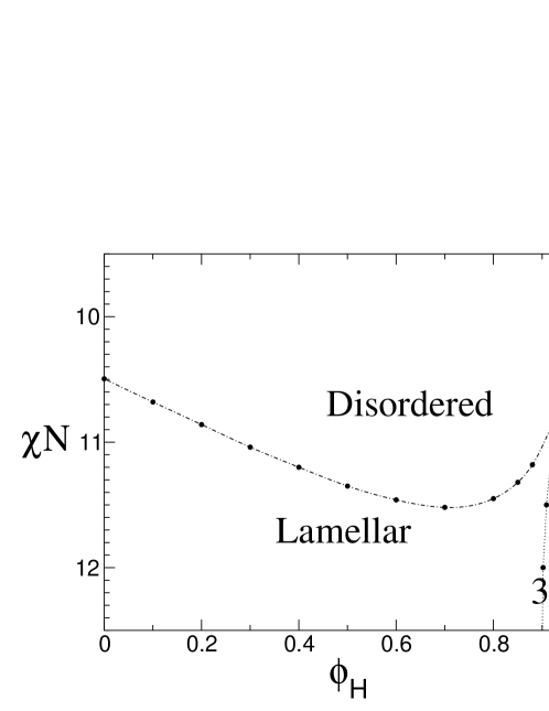
Abbildung 5: Mean-field phase diagram for a ternary symmetrical A+B+AB blend as a function of the incompatibility parameter $\chi N$ and the homopolymer volume fraction $\Phi_{H}$. The chain lengths of the copolymers is five time that of homopolymers. 2$\phi$ denotes a region of two-phase coexistence between an A-rich and a B-rich phase, 3 $\phi$ one of three-phase coexistence between an A-rich, a B-rich, and a lamellar phase. From Ref. dominik1 .

It seems plausible that fluctuations affect the Lifshitz point. If the lamellar distance is large enough that the interfaces between A and B sheets can bend around, the lamellae may rupture and form a globally disordered structure. A Ginzburg analysis reveals that the upper critical dimension of isotropic Lifshitz points is as high as 8 (see also Sec. 4.1). The lower critical dimension of isotropic Lifshitz points is $d^{*}=4$ diehl ; lifshitz_critical . Thus fluctuations destroy the transition in two and three dimensions.

Indeed, the experimentally observed phase behavior differs substantially from the mean-field phase diagram. An example is shown in Fig. 6. The Lifshitz point is destroyed, the three phase coexistence region between the lamellar phase and the demixed A-rich and B-rich phases is removed and gives way to a macroscopically mixed phase. A transmission electron micrograph of this phase is shown and compared with the structure of the lamellar phase in Fig. 7.

Abbildung 6: Experimental phase diagram of a PDMS-PE/PDMS/PE blend with copolymers about five times as long as the homopolymers. From Ref. morkved . Reproduced by permission of the Royal Society of Chemistry.

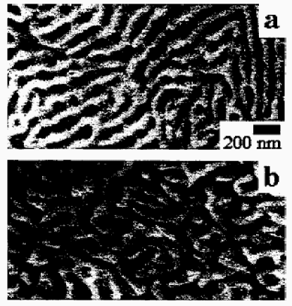
Abbildung 7: Transmission electron micrographs from symmetric PE/PEP/PE-PEP blends: (a) fluctuating lamellae (b) microemulsion phase. From Ref. morkved . Reproduced by permission of the Royal Society of Chemistry.

In order to study this effect, Düchs et al. have performed field-theoretic Monte Carlo simulations of the system of Fig. 5 dominik1 ; dominik2 ; dominik3 , in two dimensions. (For the reasons explained in Sec. 4.4.2, most of these simulations were carried out in the EP approximation). Some characteristic snapshots were already shown in Fig. 4. Here we show another series of snapshot at $\chi N=12.5$ for increasing homopolymer concentrations (Fig. 8). For all these points, the self-consistent field theory would predict an ordered lamellar phase. In the simulation, only configurations with lower homopolymer concentrations exhibit (defective) lamellar order. At higher homopolymer concentration, the order breaks up and a microemulsion emerges.

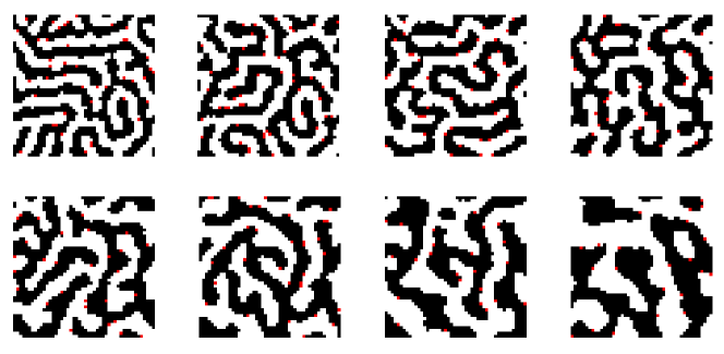
Abbildung 8: Snapshots of $\phi_{A}^{*}$ for the ternary A+B+AB system of Fig. 5 at $\chi N=12.5$ for homopolymer volume fraction $\phi_{H}=$ 0.74,0.78,0.8, 0.82 (first row from left), and 0.84, 0.86, and 0.9 (second row from left).

The phase transition can be identified by defining appropriate order parameters. We use anisotropy parameters, which are defined in terms of the Fourier transform $F({\bf q})$ of images as those shown in Fig. 8:

$$F_{n}(q)\equiv\frac{1}{2\pi}\Big{|}\int_{0}^{2\pi}\!\!\!d\phi|F({\bf q})|^{2}e^{in\phi}\Big{|}.$$ (128)

$F_{n}(q)$ is zero for isotropic (disordered) configurations and nonzero for anisotropic (lamellar) configurations. The anisotropy information can be condensed into a single dimensionless parameter

$$\bar{F}_{n}:=\frac{\int\!dqF_{n}(q)}{\sigma(q)|_{F_{n}}},$$ (129)

with the normalization

$$\sigma(q)|_{F_{n}}\equiv\Big{[}\frac{\int\!dq\>q^{2}F_{n}(q)}{\int\!dq\>F_{n}(q)}-\Big{(}\frac{\int\!dq\>q\>F_{n}(q)}{\int\!dq\>F_{n}(q)}\Big{)}^{2}\Big{]}^{1/2}.$$ (130)

Examples of anisotropy parameters are shown in Fig. 9(left). They are clearly suited to characterize the phase transition between the disordered phase at low $\chi N$ and the lamellar phase at high $\chi N$. For comparison, the same system was also examined with complex Langevin simulations. The results are shown in Fig. 9(right). The transition points are the same.

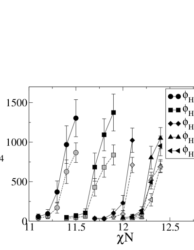
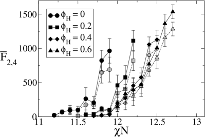
Abbildung 9: Anisotropy parameters $\bar{F}_{2}$ (solid) and $\bar{F}_{4}$ (dashed) vs. $\chi N$ for different homopolymer volume fractions $\Phi_{H}$ at the order/disorder transition. Left: From Monte Carlo Simulations (EP theory) Right: From Complex Langevin simulations. After Ref. dominik1

Unfortunately, the order of the transition could not yet determined from these simulations. In the self-consistent field theory, the transition is continuous. According to theoretical predictions brazovskii ; glenn_fluc , fluctuations shift it to lower $\chi N$ and change the order of the transition. Our simulation data are consistent both with the assumption that the transition is continuous or weakly first order. In particular, we have established that the miscibility gap between the ordered and the disordered phase is very small (data not shown).

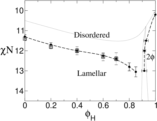
Abbildung 10: Phase diagram from simulations for the same system as above. The circles show the results from Monte Carlo simulations, the squares those from the complex Langevin simulations. The dotted lines correspond to the mean-field prediction from Fig. 5. From Ref. dominik1 .

Besides the order/disorder transition, we also need to determine the demixing transition. This was done in the grand canonical ensemble by monitoring the difference between A and B monomer densities. It exhibits a jump at the phase transition. All phase transition points are summarized in the phase diagram of Fig. 10. It is in good qualitative agreement with the experimental phase diagram of Fig. 6. In particular, we reproduce the cusp-like region of the microemulsion.

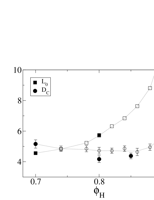
Abbildung 11: Characteristic length scales at $\chi N=12.5$ as a function of homopolymer concentration $\phi_{H}$. $D_{C}$ (circles) shows the mean (absolute) curvature radius, and $L_{0}$ the preferential length scale of layer distances, obtained from the maximum of $F_{0}(q)$ (Eq. (128)). From Ref. dominik1

The simulations allow to analyze the phase transition and the microemulsion phase in more detail. Fig. 11 compares different characteristic length scales of the system at the order/disorder transition. One length scale, $L_{0}$, is obtained from the maximum of $F_{0}(q)$ (Eq. (128)) and gives the typical distance between layers. The other is the mean absolute curvature radius $D_{C}$, and characterizes the length scale for layer bending. Whereas the typical layer distance increases with the homopolymer concentration, the curvature radius remains roughly constant. The microemulsion phase transition takes place at the value of $\phi_{H}$ where the two lines cross. Thus we can identify the mechanism by which fluctuations generate the microemulsion: The lamellae break up when their width grows larger than the length scale which characteristizes the boundary fluctuations.

To summarize, the example of homopolymer/copolymer mixtures demonstrates nicely how field-theoretic simulations can be used to study non-trivial fluctuation effects in polymer blends within the Gaussian chain model. The main advantage of these simulations is that they can be combined in a natural way with standard self-consistent field calculations. As mentioned earlier, the self-consistent field theory is one of the most powerful method for the theoretical description of polymer blends, and it is often accurate on a quantitative level. In many regions of the parameter space, fluctuations are irrelevant for large chain lengths (large ${\bar{\cal N}}$) and simulations are not necessary. Field-theoretic simulations are well suited to complement self-consistent field theories in those parameter regions where fluctuation effects become important.

7.2 Spinodal decomposition

To illustrate the application of the method to study the dynamics of collective composition fluctuations, we now consider the spontaneous phase separation (i. e., spinodal decomposition) that ensues after a quench into the miscibility gap at the critical composition, $\bar{\phi}_{A}=\bar{\phi}_{B}=1/2$, of the symmetric blend. Different time regimes can be distinguished: During the early stages, composition fluctuations are amplified. Fourier modes with a wavevector $q$ smaller than a critical value $q_{c}$ exponentially grow and modes with different wavevectors are decoupled. As the amplitude of the modes continues to grow, the composition in the domains begins to saturate and different modes begin to interact. At even later stages of phase ordering, hydrodynamics dominates the coarsening.

In the following, we restrict our attention to the early stages of spinodal decomposition. In the analysis of experiments one often uses the Landau-de Gennes functional (96). The Cahn-Hilliard-Cook theory CHC for the early stages of phase separation. This treatment predicts that Fourier modes of the composition independently evolve and increase exponentially in time with a wavevector-dependent rate, $\phi_{A}(q,t)^{2}\sim\exp[R({\bf q})t]$. Therefore, it is beneficial to expand the spatial dependence of the composition in our dynamic SCF or EP calculations in a Fourier basis of plane waves. As the linearized theory suggests a decoupling of the Fourier modes at early stages, we can describe our system by a rather small number of Fourier modes.

Using Eq. (LABEL:eq:DSCFT_RPA) one reads off the rate $R(q)$:

$$R({\bf q})=4\frac{\sqrt{{\bar{\cal N}}}k_{B}T\Lambda_{\phi}(qR_{e}^{2})}{R_{e}^{d+2}}\left[\chi N-2-\frac{(qR_{e})^{2}}{9}\right]$$ (131)

and obtains for local dynamics and Rouse-like dynamics

$$\frac{R(q)R_{e}^{2}}{D} = (qR_{e})^{2}(\chi N-2)\left[1-\left(\frac{q}{q_{c}}\right)^{2}\right]$$ (132)

$$\frac{R(q)R_{e}^{2}}{D} = (qR_{e})^{2}(\chi N-2)g(q)\left[1-\left(\frac{q}{q_{c}}\right)^{2}\right],$$ (133)

respectively, where the critical wavevector is given by $q_{c}R=\sqrt{9(\chi N-2)}$. During the early stage, composition modes with wavevectors $q<q_{c}$ will grow. In the case of local dynamics, the fastest growth occurs at $q_{c}/\sqrt{2}$. In the case of Rouse-like dynamics, the maximum of the growth rate is shifted to smaller wavevectors. The expressions above use the RPA which becomes accurate at weak segregation (WSL). Of course, the applicability of the linearized theory of spinodal decomposition using the Landau-de Gennes free energy functional is severely limited: In the ultimate vicinity of the critical point, the free energy functional does not even give an accurate description of the thermodynamic equilibrium, and the relaxation times are characterized by a non-classical, dynamical critical exponent.

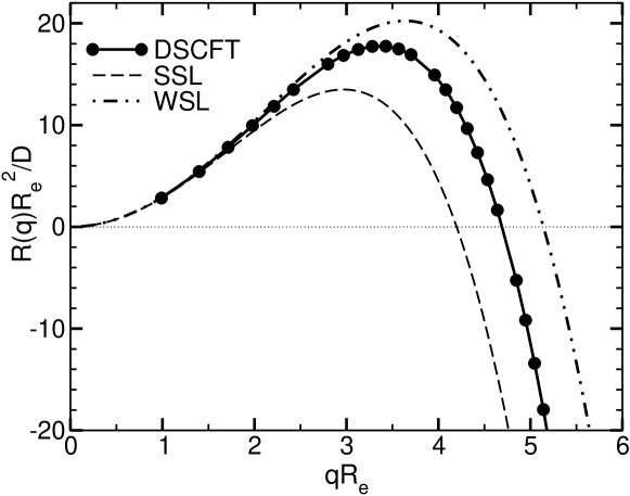
Abbildung 12: Growth rates of density modes for a quench of a symmetric mixture to $\chi N=5$. Below the critical wave vector $q_{c}$ the density modes increase spontaneously. Modes with larger wave vectors are damped. From Ref. ELLEN1 .

In the opposite limit of strong segregation (SSL) $\chi N\ll 2$, the free energy can also be expressed in terms of a square gradient functional, and one obtains $q_{c}R=\sqrt{6(\chi N-2)}$. At intermediate segregation, which is most relevant to experiments, the square-gradient approximation breaks down and there is no straightforward way to interpolate between the simple analytical expression in the weak and strong segregation limit.

The predictions of the rate $R(q)$ for the weak and the strong segregation limit are presented in Fig. 12. As expected the results of the dynamic SCF theory with a local Onsager coefficient fall between the results of the Cahn-Hilliard-Cook theory in the two limits of weak and strong segregation. Comparing the predictions for the kinetics of phase separation to experiments or simulations, it often remains unclear whether deviations are caused by approximating the free energy functional by the Landau-de Gennes expressions or the Onsager coefficient. Indeed, earlier Monte Carlo simulations found rather pronounced deviations EARL from the prediction of the Cahn-Hilliard-Cook theory CHC .

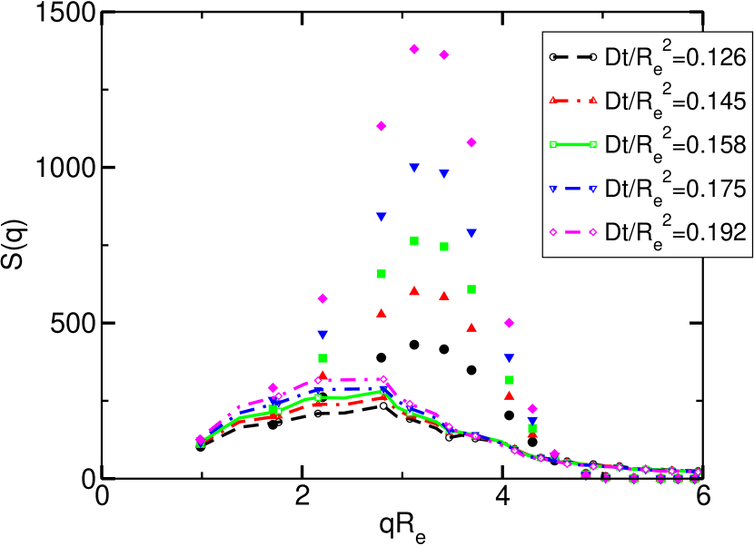
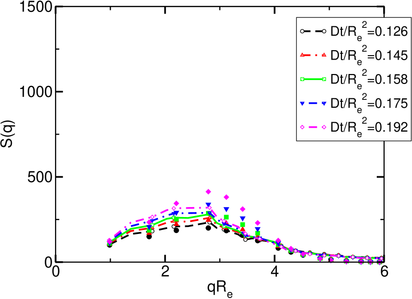
Abbildung 13: Global structure factor versus wave vector for different times for a quench from the mixed state at $\chi N=0.314$ to $\chi N=5$. Lines represent Monte Carlo results, filled symbols dynamic SCF theory results. Panel (a) compares dynamic SCF theory using a local Onsager coefficient with the Monte Carlo simulations. Local dynamics obviously overestimates the growth rate and shifts the wavevector that corresponds to maximal growth rate to larger values. Panel (b) compares dynamic SCF theory using a non-local Onsager coefficient that mimics Rouses dynamics with Monte Carlo results showing better agreement. From Ref. ELLEN1 .

To overcome this difficulty we use EP dynamics or dynamic SCF theory, which do not invoke a gradient expansion of the free energy functional and yield an accurate description of the free energy costs of composition fluctuations. Quantitatively comparing dynamical calculations to computer simulations of the bond fluctuation model BFM , we investigate the relation between the dynamics of collective composition fluctuations and the underlaying dynamics of single chains, which is encoded in the Onsager coefficient $\Lambda$. The parameters of the bond fluctuation model can be related to the coarse-grained parameters, $\chi N$, $R_{e}$ and ${\bar{\cal N}}$, of the standard SCF model and the static properties of the bond fluctuation model (e. g., the bulk phase behavior MREV ; M0 and interface properties W2 ; WET ; A0 ; andreas ) have been quantitatively compared to SCF theory. Note that the mapping between the particle-based simulation model and the SCF model does not involve any adjustable parameter: the Flory-Huggins parameter $\chi N$ is identified via the energy of mixing, the length scale is set by $R_{e}$ and the time scale is determined by the self-diffusion constant of a single polymer chain in a dense melt. All these quantities are readily measurable in the simulations. In the following example, we consider a quench to $\chi N=5$. This is a compromise: On the one hand it is sufficiently below the critical point, $\chi_{c}N=2$, such that critical composition fluctuations are not important. On the other hand the interfaces between the coexisting phases are still wide enough such that the polymers are still describable by the Gaussian chain model on the length scale of the (intrinsic) interfacial width STIFF . The chains in the bond fluctuation model comprise $N=64$ segments which corresponds to an invariant degree of polymerization, ${\bar{\cal N}}=240$. The time scale is set by $\tau=R_{e}^{2}/D=1.5\cdot 10^{7}$ Monte Carlo steps, where each segment attempts on average one random, local displacement during a Monte Carlo step. In the simulations we use a cubic system of size $L=6.35R_{e}$ and average the results over 64 independent realizations of the temperature quench.

Fig. 13 compares the time evolution of the dynamic structure factor as calculated by dynamic SCF theory using a local Onsager coefficient (panel a) and non-local Onsager coefficient (panel b) with the results of the Monte Carlo simulation. As qualitatively expected from Cahn-Hilliard-Cook theory CHC , there is a well-defined peak in the structure factor $S({\bf q},t)$

$$S({\bf q},t)\equiv\left\langle\left|\int{{\rm d}^{d}{\bf r}}\;\left(\hat{\phi}_{A}({\bf r},t)-\hat{\phi}_{B}({\bf r},t)\right)\exp(i{\bf qr})\right|^{2}\right\rangle$$ (134)

that exponentially growth with time. For these calculations we have omitted the thermal noise. Therefore, composition fluctuations with $q<q_{c}$ grow, while those with $q>q_{c}$ are damped, and the structure factor for different times exhibit a common intersection at $q_{c}$. No such well-defined critical wavevector $q_{c}$ is observed in Monte Carlo simulations or experiments, where thermal fluctuations limit the decay of fluctuations with $q>q_{c}$. Clearly, there is a sizeable difference between dynamic SCF calculations using a local Onsager coefficient and those which use a non-local $\Lambda$ corresponding to Rouse-like dynamics. The peak of the structure factor in the dynamic SCF calculations with the local Onsager coefficient grows much too fast, and also the peak in the calculations occurs at larger wavevectors compared to the Monte Carlo simulations. Apparently, the calculations with the non-local Onsager coefficient agree much better with the simulation results.

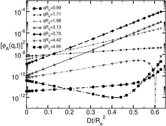
Abbildung 14: Several density modes displayed on a logarithmic scale versus time. The results were obtained through DSCFT calculations in a three dimensional system of length $L_{x}\!=\!L_{y}\!=\!L_{z}\!=\!6.35R_{e}$ using $7\!\times\!7\!\times\!7$ functions for a quench from $\chi N=0.314$ to $\chi N=5$. The expected exponential behavior during early stages of demixing is well reproduced. From Ref. ELLEN1 .

To quantify this observation, we investigate the growth (or decay) of density modes. The data in Fig. 14 show that the time evolution during the early stages of phase separation indeed is exponential and one can define a growth rate. The results for a local Onsager coefficient are presented in Fig. 12 and are bracketed by the approximations for the weak and strong segregation limits.

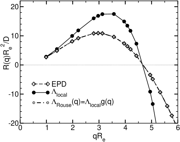
Abbildung 15: Growth rates obtained through two dimensional DSCFT calculations using local and Rouse dynamics and EPD calculations. The DSCFT results using the pair-correlation function of a homogeneous melt and the EPD results are in good agreement. From Ref. ELLEN1 .

In Fig. 15 we corroborate that the results of the dynamical SCF calculations using the non-local Onsager coefficient (114) agree with the EPD using the local Onsager coefficient (126) for the field $W$. As detailed in Sec. 5, however, the EPD calculations are computationally much less demanding.

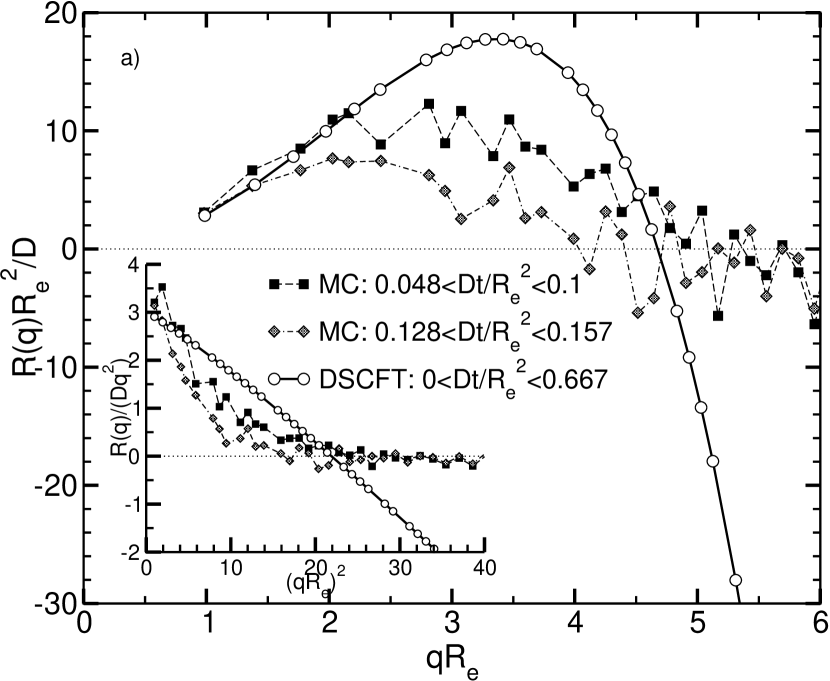
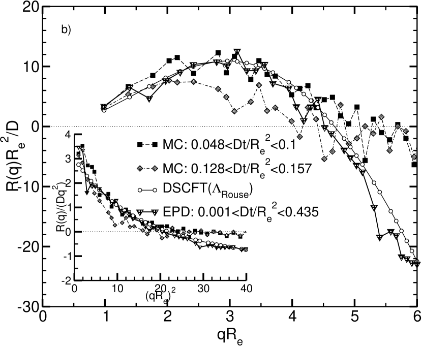
Abbildung 16: Corresponding relaxation rates to Fig. 13. Panel a) compares the Monte Carlo relaxation rates with DSCFT calculations with local dynamics. Panel b) compares Monte Carlo results with EPD and DSCFT calculations with Rouse dynamics. For earlier times good agreement in the growth region is found but Monte Carlo simulations show an earlier change in the exponential behaviour. From Ref. ELLEN1 .

The growth rates for the dynamic SCF theory with local Onsager coefficient are displayed in Fig. 16 a) and compared to the results of the Monte Carlo simulations. The maximal growth rate occurs to too large wavevectors and the growth rate for $q<q_{c}$ is too large. The Cahn plot, $R(q)/Dq^{2}$ vs.  $q^{2}$ presented in the inset, shows a linear behavior (cf. Eq. (132) in contrast to the simulations.

Much of the discrepancy between calculations and Monte Carlo simulations is removed when we employ a non-local Onsager coefficient or EPD. For $q<q_{c}$ we obtain almost quantitative agreement for the growth rate at early times. In the Monte Carlo simulations, however, deviations from the exponential growth is observed earlier than in the calculations and there is no decay of fluctuations for $q>q_{c}$ in the simulations.

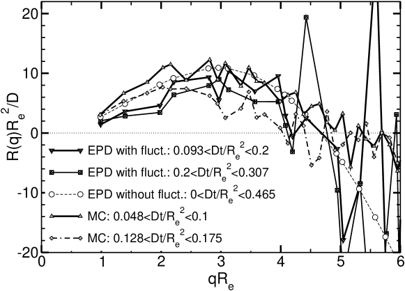
Abbildung 17: Relaxation rates obtained through Monte Carlo simulations and EPD calculations with random fluctuations for different time intervals. Fluctuations lead in both methods to an earlier change in the exponential behaviour of the increasing modes. From Ref. ELLEN1 .

Both effects can be captured if we include fluctuations in the EPD calculations. The results of EPD simulations including fluctuations are presented in Fig. 17. For $q<q_{c}$ and early times the calculations with and without fluctuations mutually agree, and resemble the simulation results. At later times, the growth rate decreases in the EPD and the simulations. For $q>q_{c}$, fluctuations do not decay in the EPD but rather adopt their finite equilibrium strength. The growth rates extracted from the EPD for $q>q_{c}$ rather mirror the fact that some modes grow and other shrink during the time window of the simulations, although the results have been averaged over 64 independent, two-dimensional EPD calculations.

The influence of the chain connectivity on the dynamics of the composition fluctuations does not only influence two-point correlation functions like the global structure factor, but it is also visible in the time evolution of composition profiles in the vicinity of a surface ELLEN2 . A description of the kinetics of phase separation is important because many multi-component polymer systems do not reach equilibrium on large length scales and the morphology of interfaces or self-assembled structures depend on processing conditions.

The example highlights that both an accurate free energy functional as well as an Onsager coefficient that describes the dynamics of the molecules are important for a quantitative description. Of course, this study has concentrated on the simplest possible scenario. The assumption of the chain conformations being in equilibrium with the instantaneous composition field and the neglect of hydrodynamics have to be address to explore the behavior of more complex systems.

8 Summary and outlook

We have briefly reviewed methods which extend the self-consistent mean-field theory in order to investigate the statics and dynamics of collective composition fluctuations in polymer blends. Within the standard model of the self-consistent field theory, the blend is described as an ensemble of Gaussian threads of extension $R_{e}$. There are two types of interactions: zero-ranged repulsions between threads of different species with strength $\chi N$ and an incompressibility constraint for the local density.

In the EP theory one regards fluctuation of the composition but still invokes a mean-field approximation for fluctuations of the total density. This approach is accurate for dense mixtures of long molecules, because composition fluctuations decouple from fluctuations of the density. The energy per monomer due to composition fluctuations is typically on the order of $\chi k_{B}T\sim k_{B}T/N$, and it is therefore much smaller than the energy of repulsive interactions (on the order $1k_{B}T$) in the polymer fluid that give rise to the incompressibility constraint. If there were a coupling between composition and density fluctuations, a better description of the repulsive hard-core interactions in the compressible mixture would be required in the first place.

Both the statics and the collective dynamics of composition fluctuations can be described by these methods, and one can expect these schemes to capture the essential features of fluctuation effects of the field theoretical model for dense polymer blends. The pronounced effects of composition fluctuations have been illustrated by studying the formation of a microemulsion dominik1 . Other situations where composition fluctuations are very important and where we expect that these methods can make straightforward contributions to our understanding are, e. g., critical points of the demixing in a polymer blend, where one observes a crossover from mean field to Ising critical behavior SCHWAHN ; HPD , or random copolymers, where a fluctuation-induced microemulsion is observed JEROME instead of macrophase separation which is predicted by mean-field theoryFML .

The application of the dynamic SCF theory MESODYN or EPD maurits ; ELLEN1 ; ELLEN2 to the collective dynamics of concentration fluctuations and the relation between the dynamics of collective concentration fluctuations and the single chain dynamics is an additional, practically important aspect. We have merely illustrated the simplest possible case – the early stages of spontaneous phase separation within a purely diffusive dynamics. In applications hydrodynamic effects HYD ; PANDERSON , shear and viscoelasticity TANAKA might become important. Even deceptively simple situations – like nucleation phenomena in binary polymer blends – still pose challenging questions BALSARA . Also the assumption of local equilibrium for the chain conformations, which allows us to use the SCF free energy functional, has to be questioned critically. Methods have been devised to incorporate some of these complications glenn2 ; VENKAT ; TANAKA ; PANDERSON , but the development in this area is still in its early stages.

Field theoretical simulations venkat ; glenn_review ; dominik1 avoid any saddle point approximation and provide a formally exact solution of the standard model of the self-consistent field theory. To this end one has to deal with a complex free energy functional as a function of the composition and density. This significantly increases the computational complexity. Moreover, for certain parameter regions, it is very difficult to obtain reliable results due to the sign problem that a complex weight imparts onto thermodynamical averages dominik1 . We have illustrated that for a dense binary blend the results of the field theoretical simulations and the EP theory agree quantitatively, i. e., density and composition fluctuation decouple dominik1 . In other systems, however, density fluctuations are of crucial importance. Let us mention two examples: (i) Field theoretical simulation methods can be used to study semi-dilute solutions glenn_review ; alexander , i. e., a compressible ensemble of Gaussian threads with repulsive interactions. In dilute solutions the chains adopt a self-avoiding walk behavior, while in semi-dilute solutions the excluded volume interactions are screened on large length scale deGennes . The very same model has been extensively studied by series expansions SER and renormalization group theory REN and those results provide an excellent testing bed to gauge the efficency of the field theoretical simulation method. (ii) It is a challenge to apply field theoretical simulations to particle-based models. This might provide valuable insight into the relation between coarse-grained parameters, $R_{e}$ and $\chi N$, of the standard model of the self-consistent field theory and the parameters (temperature, pressure/density and chain length) of a particle-based model.

Acknowledgment

It is a great pleasure to thank K. Binder, D. Düchs, V. Ganesan, G. H. Fredrickson, E. Reister, and M. Schick for their enjoyable and fruitful collaboration on this topic. Financial support was provided by the DFG under grants Mu 1674/1, Bi 314/17, and Schm 985/7 and the calculations were performed at the NIC in Jülich and the HLR Stuttgart.

- (1) R. W. Cahn, P. Haasen and E. J. Kramer, Materials Science and Technology, A Comprehensive Treatment, Vol 12, VCH, Weinheim (1993); F. Garbassi, M. Morra and E. Occhiello, Polymer Surface: From Physics to Technology, Wiley, Chichester (2000).
- (2) K. R. Shull, A. M. Mayes and T. P. Russell, Macromolecules 26, 3929 (1993); A. M. Mayes, T. P. Russell, S. K. Satija, and C. F. Majkrzak, Macromolecules 25, 6523 (1992); T. P. Russell, S. H. Anastasiadis, A. Menelle, G. P. Flecher and S. K. Satija, Macromolecules 24, 1575 (1991); P. F. Green and T. P. Russell, Macromolecules 24, 2931 (1991).
- (3) K. H. Dai, L. J. Norton and E. J. Kramer, Macromolecules 27, 1949 (1994); K. H. Dai and E. J. Kramer, Polymer 35, 157 (1994); K. H. Dai, E. J. Kramer and K. R. Shull, Macromolecules 25, 220 (1992); R. A. L. Jones, E. J. Kramer, M. H. Rafailovich and S. A. Schwarz, Phys.Rev.Lett 62, 280 (1989).
- (4) A. Budkowski, J. Klein, and L. Fetters, Macromolecules 28, 8571 (1995).
- (5) H. Tanaka, H. Hasegawa, and T. Hashimoto, Macromolecules 24, 240 (1991).
- (6) B. J. P. Jansen, S. Rastogi, H. E. H. Meijer, P. J. Lemstra, Macromolecules 34, 3998 (2001).
- (7) C. L. Tucker, P. Moldenaers, Ann. Rev. Fluid Mechanics 34, 177 (2002).
- (8) S. F. Edwards, Proc. Phys. Soc. 85, 613 (1965).
- (9) E. Helfand, Y. Tagami, J. Polym. Sci. B 9, 741 (1971); J. Chem. Phys. 56, 3592 (1971); 57, 1812 (1972); E. Helfand, A. M. Sapse, J. Chem. Phys. 62, 1327 (1975); E. Helfand, J. Chem. Phys. 62, 999 (1975).
- (10) K. M. Hong, J. Noolandi, Macromolecules 14, 727 (1981); 14, 737 (1981).
- (11) J. M. H. M. Scheutjens, G. J. Fleer, J. Chem. Phys. 83, 1619 (1979).
- (12) M. W. Matsen and M. Schick, Phys. Rev. Lett. 72, 2660 (1994); M. W. Matsen, Phys. Rev. Lett. 74, 4225 (1995); Macromolecules 28, 5765 (1995); J. Physics: Cond. Matt. 14, R21 (2001).
- (13) F. Schmid, J. Phys.: Cond. Matter 10, 8105 (1998).
- (14) P. J. Flory, J. Chem. Phys. 9, 660 (1941); H. L. Huggins, J. Chem. Phys. 9, 440 (1941).
- (15) In dimensions is independet from the number of segments per molecule and mean field theory is inaccurate, cf. A. Cavallo, M. Müller und K. Binder Europhys. Lett. 61, 214 (2003).
- (16) P. G. de Gennes. Scaling Concepts in Polymer Physics, Cornell University Press, Ithaca (1979).
- (17) O. Kratky and G. Porod, Rec. Trav. Chim. 68, 1106 (1949); N. Saito, K. Takahashi, Y. Yunoki, J. Phys. Soc. Jpn. 22, 219 (1967).
- (18) I. Szleifer, Curr. Opin. Colloid Interface Sci. 2, 416 (1997); I. Szleifer, M. A. Carignano, Adv. Chem. Phys. 1996, 94, 742 (1996).
- (19) M. Müller and M. Schick, Macromolecules 29, 8900 (1996).
- (20) M. Müller and L. G. MacDowell, Macromolecules 33, 3902 (2000); M. Müller, L. G. MacDowell, and A. Yethiraj, J. Chem. Phys. 118, 2929 (2003).
- (21) M. Müller, Macromolecules 31, 9044 (1998).
- (22) M. W. Matsen, J. Phys.: Cond. Matter 14, 21 (2002).
- (23) J. S. Rowlinson and F. L. Swinton, Liquids and liquid mixtures, Butterworths, London (1982); P. Van Konynenburg and R. L. Scott, Philos. Trans. Soc. London Series A298, 495 (1980).
- (24) A. Barker and D. Henderson, J. Chem. Phys. 47, 4714 (1967).
- (25) J. P. Hansen and I. R. McDonald, Theory of simple liquids, Academic Press (1986).
- (26) R. A. Orwoll and P. A. Arnold, Polymer-Solvent Interaction Parameter , in Physical Properties of Polymers, Handbook, J.E. Mark (ed.), Chapter 14 , AIP, Woodbury, New York (1996).
- (27) E. Reister, dissertation, Johannes Gutenberg-Universität, Mainz (2001).
- (28) E. Reister, M. Müller and K. Binder, Phys. Rev. E 64, 041804 (2001).
- (29) We note that on the right hand side of Eq. (32) the second term is smaller than the first term by a factor of and can therefore be neglected in large systems. is independent of the system size.
- (30) N. M. Maurits and J. G. E. M. Fraaije, J. Chem. Phys. 107, 5879 (1997).
- (31) W. H. Press, B. P. Flannery, S. A. Teukolsky, and W. T. Vetterling, Numerical Recipes 1986, (Cambridge Univ. Press, Cambridge, 1986).
- (32) T. Yamamoto, J. Comp. App. Math. 124, 1 (2000). X. Chen, J. Comp. App. Math. 80, 105 (1997); J.M. Martinez, J. Comp. App. Math. 124, 45 (2000).
- (33) F. Schmid, M. Müller, Macromolecules 28, 8639 (1995).
- (34) D. G. Anderson, J. Assoc. Comput. Mach. 12, 547 (1965).
- (35) V. Eyert, J. Comp. Phys. 124, 271 (1996).
- (36) R. B. Thompson, K. Ø. Rasmussen and T. Lookman, J. Chem. Phys. 120, 31 (2004).
- (37) F. Drolet and G. H. Frederickson, Phys. Rev. Lett. 83, 4317 (1999).
- (38) A. R. Mitchell and D. F. Griffiths, The Finite Difference Method in Partial Differential Equations (Wiley, Chichester, 1980).
- (39) M. D. Feit, J. A. Fleck, Jr. and A. Steiger, J. Comp. Phys. 47, 412 (1982).
- (40) K. Ø. Rasmussen and G. Kalosakas, J. Polym. Sci. B 40, 777 (2002).
- (41) D. Düchs, Dissertation Universität Bielefeld, (2003).
- (42) D. C. Morse and G. H. Fredrickson, Phys. Rev. Lett. 73, 3235 (1994).
- (43) F. Schmid and M. Müller, Macromolecules 28, 8639 (1995).
- (44) M. Müller, Macromol. Theory Simul. 8, 343 (1999).
- (45) M. Müller und K. Binder, Macromolecules 31, 8323 (1998).
- (46) V. L. Ginzburg, Sov. Phys. Solid State 1, 1824 (1960); P. G. de Gennes, J. Phys. Lett. (Paris) 38, L-441 (1977); J. F. Joanny, J. Phys. A 11, L-117 (1978); K. Binder, Phys. Rev. A 29, 341 (1984).
- (47) M. E. Fisher, Rev. Mod. Phys. 46, 587 (1974).
- (48) M. D. Gehlen, J. H. Rosedale, F. S. Bates, G. D. Wignall, K. Almdal, Phys. Rev. Lett. 68, 2452 (1992); D. Schwahn, G. Meier, K. Mortensen, and S. Janssen, J. Phys. II (France) 4, 837 (1994); H. Frielinghaus, D. Schwahn, L. Willner, and T. Springer, Physica B 241, 1022 (1998);
- (49) H. P. Deutsch and K. Binder, Macromolecules 25, 6214 (1992); J. Phys. II (France) 3 1049 (1993).
- (50) M. Müller und K. Binder, Macromolecules 28, 1825 (1995).
- (51) S. A. Brazovskii, Sov. Phys. JETP 41, 85 (1975).
- (52) G. H. Fredrickson and E. Helfand, J. Chem. Phys. 87, 697 (1987).
- (53) F. P. Buff, R. A. Lovett and F. H. Stillinger, Phys. Rev. Lett. 15, 621 (1965).
- (54) A. Werner, F. Schmid, M. Müller, K. Binder, J. Chem. Phys. 107, 8175 (1997).
- (55) A. Werner, F. Schmid, M. Müller, K. Binder, Phys. Rev. E 59, 728 (1999).
- (56) M. Müller, E. V. Albano, and K. Binder, Phys. Rev. E 62, 5281 (2000).
- (57) M. Müller und M. Schick, J. Chem. Phys. 105, 8885 (1996).
- (58) R. Holyst and M. Schick, J.Chem.Phys. 96, 7728 (1992).
- (59) C. Taupin and P. G. de Gennes, J. Phys. Chem. 86, 2294 (1982).
- (60) M. Müller und G. Gompper, Phys.Rev. E 66, 041805 (2002).
- (61) E. I. Shakhnovich and A. M. Gutin, J.Phys.France 50, 1843 (1989); G. H. Fredrickson, S. T. Milner and L. Leibler Macromolecules 25, 6341 (1992); G. H. Fredrickson and S. T. Milner, Phys. Rev. Lett. 67, 835 (1991); A. V. Subbotin and A. N. Semenov, Eur.Phys.J 7, 49 (2002).
- (62) J. Houdayer und M. Müller, Europhys.Lett. 58, 660 (2002); J. Houdayer und M. Müller, Macromolecules (in press).
- (63) A. C. Shi, J. Noolandi, and R. C. Desai, Macromolecules 29, 6487 (1996).
- (64) M. Laradji, A. C. Shi, J. Noolandi, and R. C. Desai, Phys. Rev. Lett. 78, 2577 (1997); Macromolecules 30, 3242 (1997).
- (65) I. Montvay and G. Münster, Quantum fields on the lattice, Cambridge Univ. Press, Cambridge, (1994).
- (66) J. R. Klauder, J. Phys. A 16, L317 (1983).
- (67) G. Parisi, Phys. Lett. 131B, 393 (1983).
- (68) H. Q. Lin and J. E. Hirsch, Phys. Rev. B 34, 1964 (1986).
- (69) S. A. Baeurle, Phys. Rev. Lett. 89, 080602 (2002).
- (70) A. G. Moreira, S. A. Baeurle, G. H. Fredrickson, Phys. Rev. Lett. 91, 150201 (2003).
- (71) V. Ganesan and G. H. Fredrickson, Europhys. Lett. 55, 814 (2001).
- (72) G. H. Fredrickson, V. Ganesan, F. Drolet, Macromolecules 35, 16 (2002).
- (73) G. H. Fredrickson, J. Chem. Phys. 117, 6810 (2002).
- (74) A. Alexander-Katz, A. G. Moreira, G. H. Fredrickson, J. Chem. Phys. 118, 9030 (2003).
- (75) H. Gausterer, Nucl. Phys. 642, 239 (1998).
- (76) W. J. Schoenmakers, Phys. Rev. D 36, 1859 (1987).
- (77) D. Düchs, V. Ganesan, G. H. Fredrickson, F. Schmid, Macromolecules 36, 9237 (2003).
- (78) A. Yethiraj and K. S. Schweizer, J. Chem. Phys. 98, 9080 (1993); K. S. Schweizer and A. Yethiraj, J. Chem.Phys. 98, 9053 (1993).
- (79) R. Holyst and T. A. Vilgis, J. Chem. Phys. 99, 4835 (1993); Phys. Rev. E 50, 2087 (1994).
- (80) D. Düchs, F. Schmid, NIC Series Vol. 20, p. 343 (2004).
- (81) S. Duane, A. D. Kennedy, B. J. Penleton, and D. Roweth, Physs. Lett. B 195, 216 (1987); B. Mehlig, D. W. Heermann and B. M. Forrest, Phys. Rev. B 45, 679 (1992); B. M. Forrest, U. W. Suter, J. Chem. Phys. 101, 2616 (1994).
- (82) M. Kotnis and M. Muthukumar, Macromolecules 25, 1716 (1992).
- (83) A. Chakrabarti, R. Toral, J. D. Gunton, and M. Muthukumar, Phys. Rev. Lett. 63, 2072 (1989).
- (84) C. Castellano and S. C. Glotzer, J. Chem. Phys. 103, 9363 (1995).
- (85) P. E. Rouse, J. Chem. Phys. 21, 1272 (1953).
- (86) M. Doi and S. F. Edwards, The Theory of Polymer Dynamics. Oxford University Press (1994).
- (87) K. Binder, J. Chem. Phys. 79, 6387 (1983).
- (88) P. G. de Gennes, J. Chem. Phys. 72, 4756 (1980).
- (89) P. Pincus, J. Chem. Phys. 75, 1996 (1981).
- (90) P. G. de Gennes, J. Chem. Phys. 55, 572 (1971).
- (91) P. C. Hohenberg and B. I. Halperin, Rev. Mod. Phys. 49, 435 (1977).
- (92) P. Altevogt, O. A.Evers, J. G. E. M. Fraaije, N. M. Maurits, B. A. C. van Vlimmeren, J. Mol. Struc. Theochem. 463, 139 (1999); J. G. E. M. Fraaije, J. Chem. Phys. 99, 9202 (1993).
- (93) K. G. Soga, M.J. Zuckermann, and H. Guo, Macromolecules 29, 1998 (1996), G. Besold et al.J. Polym. Sci 38, 1053 (2000).
- (94) V. Ganesan and V. Pryamitsyn, J. Chem. Phys. 118, 4345 (2003).
- (95) R. M. Hornreich, M. Luban and S. Shtrikman, Phys. Rev. Lett. 35, 1678 (1975).
- (96) R. M. Hornreich J. Magn. Magn. Mat.15, 387 (1980).
- (97) H. W. Diehl, acta physica slovaca 52, 271 (2002).
- (98) According to Ref. diehl , the lower critical dimension of an -axial Lifshitz point is given by . In our case, we have an isotropic Lifshitz point with , thus .
- (99) T. L. Morkved, B.R. Chapman, F. S. Bates, T. P. Lodge, P. Stepanek, K. Almdal, Faraday Discuss. 11, 335 (1999).
- (100) D. Düchs, F. Schmid, submitted to J. Chem. Phys. (2004).
- (101) J. W. Cahn and J. E. Hilliard, J. Chem. Phys. 28, 258 (1958); ibid 31, 668 (1959); H. E. Cook, Acta metall. 18, 297 (1970).
- (102) A. Sariban and K. Binder, Polym. Comm. 30, 205 (1989); Macromolecules 24, 578 (1991); A. Baumgärtner and D.W. Heermann, Polymer 27, 1777 (1986).
- (103) I. Carmesin and K. Kremer, Macromolecules 21, 2819 (1988). H. P. Wittmann and K. Kremer Comp. Phys. Com. 61, 309 (1990). H. P. Deutsch and K. Binder, J. Chem. Phys. 94, 2294 (1991).
- (104) M. Müller und A. Werner, J. Chem. Phys. 107, 10764 (1997).
- (105) E. Reister und M. Müller, J.Chem.Phys. 118, 8476 (2003).
- (106) N. M. Maurits, A. V. Zvelindovsky, and J. G. E. M. Fraaije, J. Chem. Phys. 108, 9150 (1998); T. Koga, K. Kawasaki, M. Takenaka, and T. Hashimoto, Physica A198, 473 (1993).
- (107) B. J. Keesta, P. C. J. van Puyvelde, P. D. Anderson and H. E. H. Heijer, Phys. Fluids 15, 2567 (2003).
- (108) H. M. Tanaka, J. Phys.: Cond. Mat 12, R207 (2000); Prog. Theo. Phys. 101, 863 (1999).
- (109) A. A. Lefebvre, J. H. Lee, N. P. Balsara, C. Vaidyanathan, J. Chem. Phys. 117, 9063 and 9074 (2002).
- (110) M. Muthukumar and B. G. Nickel, J. Chem. Phys. 86, 460 (1987).
- (111) J. des Cloizeaux and G. Jannink, Polymers in Solution: Their Modeling and Structure, Oxford Science Publications, Oxford (1990); K. F. Freed, Renormalization Group Theory of Macromolecules, Wiley, New York (1987); J. C. Le Guillou and J. Zinn-Justin, J. Phys. (France) 50, 1365 (1989); L. Schäfer, Excluded Volume Effects in Polymer Solutions, Springer, Berlin (1999).