Phase velocity and phase diffusion in periodically driven discrete state systems

Abstract

We develop a theory to calculate the effective phase diffusion coefficient and the mean phase velocity in periodically driven stochastic models with two discrete states. This theory is applied to a dichotomically driven Markovian two state system Explicit expressions for the mean phase velocity, the effective phase diffusion coefficient and the Péclet number are analytically calculated. The latter shows as a measure of phase-coherence forced synchronization of the stochastic system with respect to the periodic driving. In a second step the theory is applied to a non Markovian two state model modeling excitable systems. The results prove again stochastic synchronization to the periodic driving and are in good agreement with simulations of a stochastic FitzHugh-Nagumo system.

I Introduction

Stochastic resonance as a phenomenon of noise enhanced order in periodically driven stochastic systems has attracted considerable interest until today benzi ; cnicolis ; gammaitoni ; uspekhi . A common approach to quantify this effect are spectral based measures like the spectral power amplification and the signal to noise ratio. On the other hand stochastic resonance can also be understood as a synchronization process between the input and the response of the system gammaitoni ; ani_book . This interpretation achieves importance especially if dealing with larger amplitudes of the driving signal. Then analytical descriptions have to go beyond linear response theory.

In general two principal approaches were introduced in the past to describe the synchronization of a stochastic system by an external driving. The first one bases on the consideration of escape time densities to leave certain states of the dynamical system moss . A periodic driving modulates these densities and they exhibit maxima at times which corresponds to time scales of the external drive. “Bona fide” resonances were investigated analytically, numerically simulated and and experimentally verified, especially for symmetric bistable situations santucci ; choi ; giacomelli ; talkner .

The second approach goes back to Stratonovich who looked at synchronization of nonlinear oscillators by periodic driving in the presence of noise strato . For this purpose one adopts a phase to the nonlinear oscillators and defines statistical properties of the stochastically behaving phase. If the mean phase velocity agrees with the frequency of the driving and at the same time the phase diffusion coefficient is small then there exist in average a fixed phase relations between the driving and the output of the system.

This picture was recently transfered to models of stochastic resonance which are nonlinear but non oscillating. It was possible to prescribe a phase to overdamped bistable as well as to excitable systems which monotonously increases in time neiman ; collins ; lindner_rep . Its mean velocities and effective phase diffusion constant were used to quantify synchronization between the output and the driving input. Likewise as in stochastic resonance synchronization appears at an optimal choice of the noise intensity since the level of noise determines the characteristic times of the stochastic system.

As result one finds plateaus of the mean frequencies of the output at values which correspond to the driving frequency or multiples of it ani_book ; shulgin ; longtin2 ; zhou ; laser . These plateaus are accompanied with low phase diffusion coefficients indicating a synchronization in average. As measure of synchronization one uses the duration of locking epoches or a Péclet-number which is the ratio between the phase velocity and phase diffusion coefficient freund ; freund2 ; lai .

For bistable stochastic systems a discrete state modeling has been proven very successful in the past wiesenfeld ; loefstedt . It is based on a separation of time scales between the fast relaxation into the metastable states and the transition between these states, which happens on a slower time scale and build up a Markovian discrete dynamics talkner3 .

Also models of excitable behavior longtin ; wiesenfeld2 can be mapped on two or three state dynamics lindner ; prager1 ; prager2 . These discrete state models still set up a renewal process cox . However in difference to bistable systems they include non-exponentially distributed waiting time densities and are thus non Markovian.

These discrete state systems will be endowed with a discrete phase which is introduced in Section II. As will be shown in our paper both the Markovian and the non Markovian model exhibit phase synchronization with respect to the periodic driving for optimal noise levels. We will quantify this effect by the mean phase velocity, phase diffusion coefficient and the Péclet number. An unique approach to calculate these quantities in driven renewal models with two states will be presented in Section III. This approach is based on an envelope description of the phase freund2 ; harms .

Section IV applies the theory to bistable systems where Markovian rules were assumed for the transition between the discrete states. First results of this system with dichotomic periodic inputs were derived earlier in freund . These results were recently improved in talkner2 ; casado2 which agrees with our findings in case of Markovian dynamics.

Section V is devoted to a non Markovian two state system which models excitable behavior. Integral equations for the phase velocity and phase diffusion coefficient have to be numerically solved. Results of these computations show good quantitative agreement with numeric simulations of a stochastic periodically driven FitzHugh-Nagumo system.

II Two state models and phase

Consider a periodically driven stochastic two state system described by the probabilities ${\mathbf{p}}(t)=[p_{1}(t),p_{2}(t)]$ to be in state 1 or 2 respectively at time $t$.

In generally these dynamics can be expressed in terms of the flux operators ${\cal{J}}^{i\to j}_{t}$ by

$$\dot{p}_{1} = {\cal{J}}_{t}^{2\to 1}[{\mathbf{p}}(\cdot)]-{\cal{J}}_{t}^{1\to 2}[{\mathbf{p}}(\cdot)]$$ (1)

$$\dot{p}_{2} = {\cal{J}}_{t}^{1\to 2}[{\mathbf{p}}(\cdot)]-{\cal{J}}_{t}^{2\to 1}[{\mathbf{p}}(\cdot)]$$ (2)

The linear flux operators, which express the probability flux from state $i$ to state $j$ in terms of the occupation probabilities depend explicitly on time $t$ in a periodic way due to the periodical driving with period $T=2\pi/\Omega$,

$${\cal{J}}^{i\to j}_{t}={\cal{J}}^{i\to j}_{t+T}.$$ (3)

In the Markovian case these operators are local in time, i.e. multiplication operators,

$${\cal{J}}^{i\to j}_{t}[{\mathbf{p}}(\cdot)](t)=\gamma_{i}(t)p_{i}(t).$$

The well known two state model for bistable systems wiesenfeld which will be considered in more detail in section IV is of this type. In the non Markovian case the action of the flux operators ${\cal{J}}^{i\to j}_{t}$ on the probabilities $p_{1}$ and $p_{2}$ is non-local in time, i.e. the ${\cal{J}}^{i\to j}_{t}$ are integral operators. One example of this type is the discrete state model for excitable systems prager1 ; prager2 , whose flux operators are given by

$${\cal{J}}^{1\to 2}_{t}[{\mathbf{p}}(\cdot)](t) = \int_{t_{0}}^{t}d\tau w(t-\tau)\gamma(\tau)p_{2}(\tau)$$

$${\cal{J}}^{2\to 1}_{t}[{\mathbf{p}}(\cdot)](t) = \gamma(t)p_{2}(t)$$

Note that in this case the flux operator depend explicitly on the initial time $t_{0}$ which breaks its periodicity eq. (3). However in the asymptotic case $t_{0}\to-\infty$ this periodicity is restored. This model will be considered in section V.

Next we endow this system with a phase $\phi(t)$. Our goal is to evaluate the mean phase velocity

$$\bar{\omega}:=\lim_{t\to\infty}\frac{\left<{\phi(t)}\right>}{t}$$ (4)

as well as the effective phase diffusion constant

$$\bar{D}_{\text{eff}}:=\lim_{t\to\infty}\frac{\left<{\phi^{2}(t)}\right>-\left<{\phi(t)}\right>^{2}}{2t}.$$ (5)

These quantities are independent of the exact definition of phase, as long as the phase increases by $2\pi$ within a one cycle $1\to 2\to 1$ of the system. For the sake of notational and computational convenience we consider a phase, which increases by $2\pi$ each time the system enters state 1. Then the probabilities ${\mathbf{p}}_{k}=[p_{1,k},p_{2,k}]$ to be in state 1 or 2 respectively and to have the phase $2\pi k$ are governed by

$$\dot{p}_{1,k} = {\cal{J}}_{t}^{2\to 1}[{\mathbf{p}}_{k-1}]-{\cal{J}}_{t}^{1\to 2}[{\mathbf{p}}_{k}]$$ (6)

$$\dot{p}_{2,k} = {\cal{J}}_{t}^{1\to 2}[{\mathbf{p}}_{k}]-{\cal{J}}_{t}^{2\to 1}[{\mathbf{p}}_{k}]$$ (7)

These equations are similar to eqs. (1) and (2), however the probability influx into state 1 for a given phase $2\pi k$ comes now from states with the phase $2\pi(k-1)$.

The mean phase as well as the mean square phase are given in terms of the probabilities ${\mathbf{p}}_{k}$ by

$$\left<{\phi(t)}\right> = \sum_{k=-\infty}^{\infty}2\pi k(p_{1,k}(t)+p_{2,k}(t))$$

$$\left<{\phi^{2}(t)}\right> = \sum_{k=-\infty}^{\infty}4\pi^{2}k^{2}(p_{1,k}(t)+p_{2,k}(t))$$

The instantaneous mean phase velocity $\omega(t)$ and instantaneous mean phase diffusion $D_{\text{eff}}(t)$ are then defined as

$$\omega(t) = \frac{d}{dt}\left<{\phi(t)}\right>$$ (8)

$$D_{\text{eff}}(t) = \frac{1}{2}\frac{d}{dt}\Big{[}\left<{\phi^{2}(t)}\right>-\left<{\phi(t)}\right>^{2}\Big{]}.$$ (9)

Asymptotically, i.e. for the initial time $t_{0}\to-\infty$, the phase $\phi=2\pi k$ will undergo a diffusional motion talkner2 with periodically varying effective phase velocity $\omega(t)$ and effective diffusion coefficient $D_{\text{eff}}(t)$. In this asymptotic regime the mean phase velocity eq. (4) and effective phase diffusion constant eq. (5) can be expressed as the time average over one period of the external driving of the time dependent phase velocity and diffusion constant,

$$\bar{\omega}=\frac{1}{T}\int_{0}^{T}dt\omega(t)\quad\text{and}\quad\bar{D}_{\text{eff}}=\frac{1}{T}\int_{0}^{T}dtD_{\text{eff}}(t)$$ (10)

Although the phase velocity and effective phase diffusion constant eqs. (8) and (9) have a periodic asymptotic behavior, the equations (6) and (7) which govern the probabilities $p_{1,k}$ and $p_{2,k}$ obviously have no asymptotic solutions.

III General theory

Our aim is to relate the asymptotic phase velocity and effective phase diffusion constant eqs. (10) to the microscopic dynamics eqs. (6) and (7). To this end we introduce a continuous phase distribution ${\cal{P}}(\phi,t)$ as the envelope of the discrete phase distribution $p_{1,k}$ and $p_{2,k}$ freund2 ; harms by defining its values at integer multiples of $2\pi$ as

$${\cal{P}}(\phi=2\pi k,t):=p_{1,k}(t)+p_{2,k}(t).$$ (11)

The diffusional motion of the phase $\phi$ requires its distribution ${\cal{P}}(\phi)$ to obey the Fokker-Planck equation

$$\frac{\partial}{\partial{t}}{\cal{P}}(\phi,t)=\frac{\partial}{\partial{\phi}}(-\omega(t)+D_{\text{eff}}(t)\frac{\partial}{\partial{\phi}}){\cal{P}}(\phi,t).$$ (12)

To establish the relation between $\omega(t)$ and $D_{\text{eff}}(t)$ and the microscopic dynamics eqs.(6) and (7) we expand $p_{1,k}$ and $p_{2,k}$ according to

$$p_{i,k}(t) = \sum_{n=0}^{\infty}q_{i}^{(n)}(t)\frac{\partial^{n}}{\partial{\phi}^{n}}{\cal{P}}(\phi,t)\Big{|}_{\phi=2\pi k},\quad i=1,2\quad$$ (13)

This expansion describes how the probability to be in state 1 or 2 for a given phase $k$ at time $t$, $p_{1,k}(t)$ and $p_{2,k}(t)$ respectively, is related to the total probability to have a phase $2\pi k$, ${\cal{P}}(2\pi k,t)$ and its gradients.

The total probability $p_{1,k}(t)+p_{2,k}(t)$ to have a phase $2\pi k$ neglecting the internal state 1 or 2 is related to the continuous phase distribution by the defining eq. (11), which in turn implies

$$q_{1}^{(0)}(t)+q_{2}^{(0)}(t) = 1$$ (14)

$$q_{1}^{(n)}(t)+q_{2}^{(n)}(t) = 0\quad\text{for }n\geq 1.$$

Inserting the Ansatz eq. (13) into the master eq. (6) and (7), using the Fokker-Planck equation (12) for the phase and considering the coefficients of the different derivatives $\partial^{n}/\partial\phi^{n}{\cal{P}}(\phi,t)$ eventually leads to (cf. appendix A)

$$\dot{\mathbf{q}}^{(0)} = {\mathbf{M}}_{t}[{\mathbf{q}}^{(0)}]$$ (15)

$$\dot{\mathbf{q}}^{(1)} = {\mathbf{M}}_{t}[{\mathbf{q}}^{(1)}+c^{(1)}_{t}{\mathbf{q}}^{(0)}]-2\pi{\mathbf{J}}^{\text{in}}_{t}[{\mathbf{q}}^{(0)}]+\omega(\cdot){\mathbf{q}}^{(0)}$$ (16)

$$\dot{\mathbf{q}}^{(2)} = {\mathbf{M}}_{t}[{\mathbf{q}}^{(2)}+c^{(1)}_{t}{\mathbf{q}}^{(1)}+c^{(2)}_{t}{\mathbf{q}}^{(0)}]-2\pi{\mathbf{J}}^{\text{in}}_{t}[{\mathbf{q}}^{(1)}+(c_{t}^{(1)}-\pi){\mathbf{q}}^{(0)}]+\omega(\cdot){\mathbf{q}}^{(1)}-D_{\text{eff}}(\cdot){\mathbf{q}}^{(0)}$$ (17)

where we have introduced the master operator

$${\mathbf{M}}_{t}[\cdot]=\begin{pmatrix}{\cal{J}}_{t}^{2\to 1}[\cdot]-{\cal{J}}_{t}^{1\to 2}[\cdot]\\ {\cal{J}}_{t}^{1\to 2}[\cdot]-{\cal{J}}_{t}^{2\to 1}[\cdot]\end{pmatrix}.$$

The operator

$${\mathbf{J}}^{\text{in}}_{t}[\cdot]=\begin{pmatrix}{\cal{J}}_{t}^{2\to 1}[\cdot]\\ 0\end{pmatrix}$$

accounts for the influx into state 1 and we introduced

$$c^{(1)}_{t}(t^{\prime}) = \int_{t^{\prime}}^{t}d\tau\omega_{0}(\tau)$$

$$c^{(2)}_{t}(t^{\prime}) = -\int_{t^{\prime}}^{t}d\tau D_{0}(\tau)+\omega_{0}(t)\int_{t^{\prime}}^{t}d\tau(t-\tau)\omega_{0}(\tau).$$

${\mathbf{q}}^{(0)}$ in eq. (15) shows the same dynamics as ${\mathbf{p}}$ in the two state system without phase eqs. (1) and (2), which one would also expect as this term corresponds to an equipartition of phases ${\cal{P}}(\phi,t)=\text{const}$ in the expansion eq. (13). The higher order terms ${\mathbf{q}}^{(n)}$ are corrections which emerge due to the fact that we are considering a non equipartition of phases resulting in drift and diffusion.

Interestingly if the action of the flux operators on the probabilities is local in time, i.e. in the Markovian case the terms containing the $c_{t}^{(i)}$ are zero, as $c_{t}^{(i)}(t)=0$, and therefore the dynamics of the ${\mathbf{q}}^{(i)}$ considerably simplifies.

By summing up both components of the vectorial eqs. (16) and (17), using the normalization condition eq. (14) and the fact that $({\mathbf{M}}_{t})_{1}+({\mathbf{M}}_{t})_{2}=0$ we arrive at

$$\omega(t) = 2\pi{\cal{J}}^{2\to 1}_{t}[{\mathbf{q}}^{(0)}](t)$$ (18)

$$D_{\text{eff}}(t) = 2\pi{\cal{J}}^{2\to 1}_{t}[-{\mathbf{q}}^{(1)}+(\pi-c_{t}^{(1)}){\mathbf{q}}^{(0)}](t)$$ (19)

$$= \pi\omega(t)+2\pi{\cal{J}}^{2\to 1}_{t}[-{\mathbf{q}}^{(1)}-c_{t}^{(1)}{\mathbf{q}}^{(0)}](t)$$

The asymptotic mean phase velocity $\bar{\omega}$ and the asymptotic effective phase diffusion constant $\bar{D}_{\text{eff}}$ can then be determined from the asymptotic (cyclo stationary) solutions of eqs. (15) and (16). Therefore, the calculation of the asymptotic effective diffusion constant is reduced to the solution of a cyclo stationary problem, which in general is simpler that solving the whole non stationary equations (6) and (7) with some initial conditions and then taking the asymptotic limit in eq. (5).

In the following the mean phase velocity and effective phase diffusion constant will be considered for two different models, namely a Markovian model wiesenfeld , which approximates bistable systems and a non-Markovian model prager2 , which serves as an approximate description for excitable systems. For the dichotomically driven Markovian case the mean phase velocity and effective phase diffusion constant can be explicitly calculated, while for the non-Markovian case solutions can only be obtained numerically.

IV A Markovian two state model

We consider now a Markovian two state system with periodically modulated rates $\gamma_{2}(t)$ and $\gamma_{1}(t)$. Its flux operator ${\cal{J}}^{1\to 2}$ and ${\cal{J}}^{2\to 1}$ are given by

$${\cal{J}}_{t}^{1\to 2}[{\mathbf{p}}](t)=\gamma_{1}(t)p_{1}(t)\quad\text{and}\quad{\cal{J}}_{t}^{2\to 1}[{\mathbf{p}}](t)=\gamma_{2}(t)p_{2}(t)$$

In this Markovian case, the equations, which govern the evolution of ${\mathbf{q}}^{(i)}(t)$ greatly simplify due to the fact that $c^{(i)}_{t}(t)=0$. Eqs. (18) and (19) reduce to

$$\omega(t) = 2\pi\gamma_{2}(t)q_{2}^{(0)}(t)$$

$$D_{\text{eff}}(t) = 2\pi^{2}\gamma_{2}(t)q_{2}^{(0)}(t)-2\pi\gamma_{2}(t)q_{2}^{(1)}(t).$$

The equations for $q_{2}^{(0)}(t)$ and $q_{2}^{(1)}(t)$ are given by

$$\dot{q}_{2}^{(0)}(t) = \gamma_{1}(t)q_{1}^{(0)}(t)-\gamma_{2}(t)q_{2}^{(0)}(t)$$ (20)

$$\dot{q}_{2}^{(1)}(t) = \gamma_{1}(t)q_{1}^{(1)}(t)-\gamma_{2}(t)q_{2}^{(1)}(t)+\omega(t)q_{2}^{(0)}(t)\;\;\;\;$$ (21)

Eqs. (20) and (21) can be readily solved by the method of variation of constants, using $q_{1}^{(0)}(t)=1-q_{2}^{(0)}(t)$ and $q_{1}^{(1)}(t)=-q_{2}^{(1)}(t)$ (cf. eq. (14)). The asymptotic periodic solutions eventually read

$$q_{2}^{(0)}(t) = \frac{\int_{0}^{T}d\tau\gamma_{1}(t-\tau)\exp(-s(\tau,t))}{1-\exp(-s(T,t))}$$ (22)

$$q_{2}^{(1)}(t) = \frac{\int_{0}^{T}d\tau\omega(t-\tau)q_{2}^{(0)}(t-\tau)\exp(-s(\tau,t))}{1-\exp(-s(T,t))}\;\;\;$$ (23)

where $s(\tau,t):=\int_{t-\tau}^{t}d\tau^{\prime}(\gamma_{1}(\tau^{\prime})+\gamma_{2}(\tau^{\prime}))$. Note that $s(T,t)$ does no longer depend on $t$.

For a dichotomic symmetric driving with period $T=2\pi/\omega$,

$$\gamma_{1}(t)=\left\{\begin{array}[]{ll}r_{1}&\text{if }t\in[nT,(n+\frac{1}{2})T)\\ r_{2}&\text{if }t\in[(n+\frac{1}{2})T,(n+1)T)\end{array}\right.$$

and vice versa for $\gamma_{2}(t)$ eqs. (22) and (23) can be readily evaluated leading after some cumbersome algebra to the mean phase velocity and effective phase diffusion constant

$$\bar{\omega} = \omega_{0}+\alpha\Omega\tanh R$$ (25)

and

$$\bar{D}_{\text{eff}} = \pi\omega_{0}\big{[}\frac{1}{2}+\alpha(\frac{1}{2}+\cosh^{-2}R)\big{]}+$$

$$\pi\alpha\Omega\tanh R\big{[}-1+\alpha(\frac{1}{2}\cosh^{-2}R+1)\big{]}$$

where we have introduced the mean phase velocity without driving $\omega_{0}:=2\pi/(\frac{1}{r_{1}}+\frac{1}{r_{2}})$, a quantifier for the driving strength $\alpha=\frac{(r_{1}-r_{2})^{2}}{(r_{1}+r_{2})^{2}}$ and some ratio between inner time scale and driving frequency $R=\frac{\pi(r_{1}+r_{2})}{2\Omega}$.

Without signal, i.e. $\alpha=0$ eq. (IV) reduces to $\bar{D}_{\text{eff}}=\pi\omega_{0}$, which agrees with the result in cox , $\bar{D}_{\text{eff}}=(2\pi)^{2}/2(\left<{t^{2}}\right>-\left<{t}\right>^{2})/\left<{t}\right>^{3}$.

Next we consider the small and large noise limits of the phase velocity $\bar{\omega}$ and phase diffusion constant $\bar{D}_{\text{eff}}$ for the case of Arrhenius rates $r_{1/2}=r_{0}\exp(-\frac{\Delta U\pm A}{D})$. In this case $\alpha=\tanh^{2}(\frac{A}{D})$.

If for a fixed driving frequency the noise level is sufficiently small such that $R\ll 1$ eqs. (25) and (IV) reduce to

$$\bar{\omega} \approx \omega_{0}+\alpha\Omega R=\frac{\pi}{2}(r_{1}+r_{2})\approx\frac{\pi}{2}r_{2}$$

$$\bar{D}_{\text{eff}} \approx \pi\omega_{0}(\frac{1}{2}+\frac{3}{2}\alpha)+\pi\alpha\Omega R(-1+\frac{3}{2}\alpha)$$

$$= \frac{\pi^{2}}{4}(r_{1}+r_{2})\approx\frac{\pi^{2}}{4}r_{2}$$

where in the last step we used the fact that $r_{2}$ dominates $r_{1}$ for small noise levels. Therefore, at the level of phase velocity and phase diffusion, the process behaves like a process without driving whose rates are both equal to $\frac{r_{2}}{2}$.

On the other hand if the noise level is large and the driving frequency is small compared to $\alpha_{0}$ such that $R\gg 1$ we get

$$\bar{\omega} \approx \omega_{0}+\alpha\Omega=2\pi\frac{r_{1}r_{2}}{r_{1}+r_{2}}+\Omega\frac{(r_{1}-r_{2})^{2}}{(r_{1}+r_{2})^{2}}$$

$$\bar{D}_{\text{eff}} \approx \frac{\pi}{2}\omega_{0}(1+\alpha)+\pi\alpha\Omega(-1+\alpha)$$

$$= 2\pi^{2}\frac{r_{1}r_{2}(r_{1}^{2}+r_{2}^{2})}{(r_{1}+r_{2})^{3}}-4\pi\Omega\frac{(r_{1}-r_{2})^{2}}{(r_{1}+r_{2})^{4}}$$

The first terms in these expressions correspond to a process without driving with one rate equal to $r_{1}$ and the other equal to $r_{2}$, while the second terms are corrections which vanish for vanishing driving frequency.

Between these regions we have a competing behavior. If for a fixed driving amplitude $A$, the noise strength $D$ is sufficiently small, such that $\alpha\approx 1$ and $\omega_{0}\approx 0$, and simultaneously, for a fixed driving frequency $\Omega$, $D$ is sufficiently large such that $R\gg 1$, i.e. $\tanh R\approx 1$ we have

$$\bar{\omega} \approx \Omega$$

$$\bar{D}_{\text{eff}} \approx 0$$

i.e. frequency and phase locking occur.

Having calculated the effective diffusion coefficient and the mean phase velocity we can evaluate the Péclet number

$${\rm Pe}:=\frac{2\pi\bar{\omega}}{\bar{D}_{\text{eff}}}$$ (27)

which is a measure of the phase coherence.

In Fig.1 the theoretical results eqs. (25),(IV) and (27) are compared to simulations of the driven two state system. To compute these results we have modified an algorithm presented in gibson taking into account that the transition rates are piecewise constant in time due to the dichotomic driving. Let us assume we start at time $t$ in state $1$ and the input defines the rate to have the value $r_{1}$. Then we draw a random number $\tau$ according to the corresponding waiting time distribution $w_{r_{1}}(\tau)=r_{1}\exp(-r_{1}\tau)$. If $t+\tau$ is smaller then the time $t_{s}$ of the next switching of the input we set the running time to $t+\tau$ and perform the transition to the second state of the system. This state $2$ will be left with rate $r_{2}$ and we proceed accordingly. Contrary if during the interval $[t,t+\tau]$ a switching of the input occurs we set the running time equal to the switching time $t_{s}$ but remain in state $1$. After switching of the input the rate for leaving state $1$ is now $r_{2}$ and we proceed by drawing a new waiting time according to the new density $w_{r_{2}}(\tau)=r_{2}\exp(-r_{2}\tau)$.

Figure 1: Mean phase velocity $\omega_{0}$ (top), effective phase diffusion constant $D_{0}$ (middle) and Péclet number ${\rm Pe}$ (bottom) of the Markovian model for different values of the driving amplitude.
Symbols are simulation data of the two state system, lines according to eq. (25), (IV) and (27), respectively. Other parameters: $r_{0}=1$ and $\Delta U=0.25$, $\Omega=0.001\pi$. The deviation between theory and simulations in the Péclet number for low noise intensities is due to limited simulation time.

The Péclet number shows a maximum as a function of noise strength, indicating stochastic resonance. For a strong driving, it varies over several orders of magnitude with varying noise strength $D$. Interestingly the Péclet number shows also a non monotonic behavior as a function of driving frequency for a fixed noise level, i.e. using this number as a measure of the quality of the response to the external signal we discover a “bona fide “ resonance (Fig. 2).

Figure 2: Péclet number ${\rm Pe}$ of the Markovian model as a function of driving frequency $\Omega$ for different noise values. $A=0.2$, other parameters as in Fig. 1. The inset shows the driving frequency at the maximum Péclet number as a function of noise strength (solid line) compared to the intrinsic frequency $\Gamma$ without driving ($A=0$) (dashed line).

V Excitable systems

In this section we consider the phase velocity and diffusion of a non Markovian model prager2 . This two state model mimics the dynamics of an excitable systems by dividing it into an excitation step and the evolution along the excitation loop. Its dynamics is given by

$$\dot{p}_{1}(t) = \gamma(t)p_{2}(t)-\int_{t_{0}}^{t}d\tau w(t-\tau)\gamma(\tau)p_{2}(\tau)$$ (28)

$$\dot{p}_{2}(t) = -\gamma(t)p_{2}(t)+\int_{t_{0}}^{t}d\tau w(t-\tau)\gamma(\tau)p_{2}(\tau).\;\;$$ (29)

with initial conditions

$$p_{1}(t_{0})=0\quad\text{ and }\quad p_{2}(t_{0})=1.$$ (30)

State 2 represents the rest state, in which we start at initial time $t_{0}$ >From there the system is excited due to noise and the external periodic subthreshold signal, leading a rate process with rate $\gamma(t)$, which depends periodically on time. This Markovian excitation step is described by

$${\cal{J}}_{t}^{2\to 1}[{\mathbf{p}}](t) = \gamma(t)p_{2}(t).$$ (31)

State 1 accounts for the motion on the excitation loop on which the systems spends a time distributed according to the waiting time distribution $w(\tau)$, which is assumed not to depend on the weak external driving. The flux from state 1 back to state 2 is then expressed in terms of the flux from state 2 to state 1 at prior times $\tau$ between $t_{0}$ to $t$ $\gamma(\tau)p_{2}(\tau)$, which renders the description non Markovian, leading to the flux operator

$${\cal{J}}_{t}^{1\to 2}[{\mathbf{p}}](t) = \int_{t_{0}}^{t}d\tau w(t-\tau)\gamma(\tau)p_{2}(\tau).$$ (32)

Note that this operator depends explicitly on the initial time $t_{0}$.

To calculate the asymptotic periodic solution it will be useful to first formally integrate eqs. (28), (29) taking into account the initial conditions (30) and then taking the initial time $t_{0}$ to $-\infty$. The resulting equations are

$$p_{1}(t) = \int_{0}^{\infty}d\tau z(\tau)\gamma(t-\tau)p_{2}(t-\tau)$$ (33)

$$p_{2}(t) = 1-\int_{0}^{\infty}d\tau z(\tau)\gamma(t-\tau)p_{2}(t-\tau).$$ (34)

where $z(\tau)=1-\int_{0}^{\tau}d\tau^{\prime}w(\tau^{\prime})$ is the probability to spent a time longer than $\tau$ on the excitation loop. By differentiating these equations with respect to $t$ one recovers the original eqs. (28) and (29) in the limit $t_{0}\to-\infty$ comment .

If we take into account the phase eq. (34) has to be replaced by

$$p_{(1,k)}(t) = \int_{0}^{\infty}d\tau z(\tau)\gamma(t-\tau)p_{(2,k-1)}(t-\tau).$$ (35)

We also have to take care of the flux operator ${\cal{J}}_{t}^{1\to 2}$ which in the asymptotic case is given by (cf. eq. (32))

$${\cal{J}}_{t}^{1\to 2}[{\mathbf{p}}](t) = \int_{0}^{\infty}d\tau w(\tau)\gamma(t-\tau)p_{2}(t-\tau).$$ (36)

In the following we assume a fixed waiting time $T$ on the excitation loop, i.e. $w(\tau)=\delta(T-\tau)$ and $z(\tau)=\theta(T-\tau)$. Such an assumption is justified in the low noise limit for e.g. FitzHugh-Nagumo models (cf. Fig. 6). In this case eq. (36) simplifies to

$${\cal{J}}_{t}^{1\to 2}[{\mathbf{p}}](t) = \gamma(t-T)p_{2}(t-T).$$ (37)

Then, according to eqs. (18) and (19), the time dependent phase velocity $\omega_{0}(t)$ and effective phase diffusion constant $D_{0}(t)$ are given by

$$\omega(t) = 2\pi\gamma(t)q_{2}^{(0)}(t)$$ (38)

$$D_{\text{eff}}(t) = -2\pi\gamma(t)q_{2}^{(1)}(t)+2\pi^{2}\gamma(t)q_{2}^{(0)}(t),$$

which are the same expressions as in the Markovian case, as the flux operator ${\cal{J}}_{t}^{2\to 1}$ is the same. However the equations governing the ${\mathbf{q}}^{(i)}$ are different. Following the same procedure we used to treat eqs. (6) and (7) eq. (35) together with normalization the condition (14) leads to

$$1-q_{2}^{(0)}(t) = \int_{0}^{T}d\tau\gamma(t-\tau)q_{2}^{(0)}(t-\tau)$$ (39)

$$-q_{2}^{(1)}(t) = \int_{0}^{T}d\tau\gamma(t-\tau)q_{2}^{(1)}(t-\tau)$$

$$+\int_{0}^{T}d\tau\gamma(t-\tau)q_{2}^{(0)}(t-\tau)(\int_{0}^{\tau}d\tau^{\prime}\omega(t-\tau^{\prime})-2\pi).$$

The periodic solutions of eqs. (39), (V) can be numerically obtained in Fourier space using a linear solver like LAPACK.

To investigate the role of noise on the synchronization in excitable system we choose an Arrhenius type excitation rate for the transition from the rest state $2$ onto the excitation loop $1$. We further assume that the external driving acts as a modulation of the potential barrier. Again we consider a dichotomic periodic driving, i.e. the excitation rate $\gamma(t)$ periodically switches between the two values $r_{1}=r_{0}\exp(-(\Delta U-A)/D)$ and $r_{2}=r_{0}\exp(-(\Delta U+A)/D)$.

The resulting phase velocity, effective phase diffusion and Péclet number as a function of noise strength $D$ are shown in Fig. 3. As in the case of bistable systems we observe frequency and phase locking, however there exist preferred driving frequencies for which high synchronization is achieved and other frequencies which show no synchronization at all.

The Péclet number shows a local maximum at a finite noise strength. Contrary to the bistable situation however, the phase diffusion constant decreases again and the Péclet number therefore increases for large noise levels. This behavior is originated in the fixed time $T$ on the excitation loop. Taking into account the high rate and therefore small waiting time and variance of the excitation step for high noise levels this leads to a low variance of the spiking, which implies a low diffusion of the phase. We mention that this low phase diffusion does not imply synchronization since the frequencies are not locked. Also we note that in real excitable systems the behavior differs. For higher noise levels the time spent on the excitation loop will have a variance in these systems which yields an increasing phase diffusion with growing noise.

Figure 3: Mean phase velocity $\bar{\omega}$ (top, inset), effective phase diffusion constant $\bar{D}_{\text{eff}}$ (top) and Péclet number ${\rm Pe}$ (bottom) of the non Markovian model for different values of the driving frequency $\Omega$.
Symbols are simulation data of the two state system, lines according to numerical evaluation of the theory. Other parameters: $T=2800$, $r_{0}=0.0044$, $\Delta U=5.6\cdot 10^{-5}$ and $A=5.0\cdot 10^{-5}$.

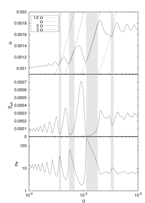
Figure 4: Mean phase velocity $\bar{\omega}$ (top), effective phase diffusion constant $\bar{D}_{\text{eff}}$ (middle) and Péclet number Pe (bottom) of the non Markovian model as a function of driving frequency $\Omega$ for $D=0.00001$. The shaded regions are a guide for the eye and represent regions of frequency synchronization. In these regions we also find a small effective phase diffusion and therefore a high Péclet number. Other parameters: $T=2800$, $r_{0}=0.0044$, $\Delta U=5.6\cdot 10^{-5}$ and $A=5.0\cdot 10^{-5}$.

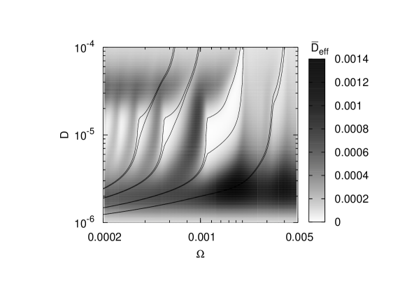
Figure 5: Effective phase diffusion constant ${\bar{D}_{\text{eff}}}$ of the non Markovian model, as a function of driving frequency $\Omega$ and noise level $D$. The black lines show regions of frequency locking $(1-\epsilon)\Omega<n\bar{\omega}<(1+\epsilon)\Omega$, $\epsilon=0.01$ with (from left to right) $n=3,2,1,\frac{1}{2}$. These regions of frequency locking coincide with low phase diffusion. Other parameters as in Figs. 3 and 4.

As seen in Fig.3 the synchronization behavior strongly depends on the driving frequency. To further analyze this effect we have plotted in Fig.4 the mean phase velocity, phase diffusion coefficient and the Péclet number as function of the driving frequency. They show a complex sequence of different locking regions between the driving and the system’s response parmananda ; lee , represented by shaded regions. In these locking regions the effective phase diffusion is small (see Fig.5). We mention that the maximal frequency of the excitable system is $\bar{\omega}_{\rm max}=2\pi/T$ where $T$ is the time on the excitation loop. There can not be $1:1$ synchronization for $\Omega>\bar{\omega}_{max}$.

Let us for a moment assume the extreme case where one excitation rate $r_{1}$ is infinity and the other $r_{2}$ is zero. Then the system remains in the rest state as long as the input causes the vanishing excitation rate. After the input changes the system immediately starts with the excitation loop where it stays the time $T$. For a $1:1$ locking this time $T$ must be larger than half the period but smaller the full period $2\pi/\Omega$ of the driving. Otherwise, if the duration of the excitation loop would be smaller than half the period the system returns to the rest state where it immediately starts a new excitation. In consequence $1:n$ locking where the output frequency is $n$ times higher than the input frequency occurs if the period of the driving is between $(n-1/2)T$ and $nT$.

The opposite case where a fast input locks a slow output occur if multiple periods of the input fit into the excitation time. During the excitation the system does not respond to the changes of the input. If the input has the phase with long waiting time after the system has completed the excitation loop, it has to wait until the input changes to the phase with the small waiting time, leading to a $n:1$ synchronization where $n$ is the number of signal periods which fit into the excitation time $T$.

However if the system finds the high excitation rate after excursion it immediately starts a new excitation loop and repeats these until it will find the phase with long waiting times. This yields a $n:m$ frequency locking with $n>m$. Note that there are no $n:m$ locking modes with $n<m$ except the $1:m$ modes described above.

Realistic noise dependent time scales will weaken the extreme behavior of the situation considered above. There are two competing effects namely increasing the noise increases $r_{1}$ as well as $r_{2}$ while decreasing the noise increases the ratio between $r_{1}$ and $r_{2}$ and therefore the effect of the driving. Hence, we find synchronization in a finite window of noise intensities where the two activation times enclose the time $T$ on the excitation loop,

$$\frac{1}{r_{1}}\ll T\ll\frac{1}{r_{2}}.$$ (41)

We point out that this latter time plays the essential role within the synchronization process, i.e. this time scale and the period of the external drive have to be tuned appropriately to get phase synchronization. Noise as well as the amplitude of driving define the two excitation rates and have to be chosen such that eq. (41) is optimally fulfilled, i.e. that the input acts as much as possible as a on-off switch on the excitation process. A deviation from this extremal behavior leads to a narrowing of the driving frequency windows amenable to frequency locking and a shift of these windows to lower frequencies.

Finally we compare the theory to a dynamical system with excitable dynamics, namely the FHN model fhn1 ; fhn2

$$\dot{x} = x-x^{3}-y+\sqrt{2D}\xi(t)$$

$$\dot{y} = \epsilon(x+a_{0}-a_{1}y-s(t))$$ (42)

This system is driven by a dichotomic periodic signal $s(t)$ with values $\pm A$ where $A=0.015$. Setting $a_{0}=0.405$ and $a_{1}=0.5$ the system is in the excitable regime for both values of the signal, i.e. the signal is a sub-threshold signal. We further consider a strong time scale separation $\epsilon=0.001$ as well as a small noise level $D=10^{-5}$. The phase of the system is defined to increase by $2\pi$ each time a spike is generated. From simulations of the inter spike interval distribution (see Fig. 6) for constant signal $\pm A$ we find the corresponding parameters of the two state model to be $T\approx 2620$, $r_{1}\approx 0.0087$ and $r_{2}\approx 8.310^{-8}$ .

Figure 6: Inter spike interval distribution of the FHN system eqs. (V) with constant signal $s(t)=0.04$ for a low noise level $D=10^{-5}$ and strong time scale separation $\epsilon=0.001$. Other parameters see text.

The results for the phase velocity $\bar{\omega}$ and effective phase diffusion constant $\bar{D}_{\text{eff}}$ for the FHN system (numerical simulation of eqs. (V)) and the theory eqs. (38) and (V) are shown in Fig. 7. They show a good qualitative agreement over a large range of driving frequencies. The deviation for larger driving frequencies is due to the fact that, in contrast to the assumptions of our two state model, the time $T$ spent on the excitation loop depends if however only weakly on the driving.

Figure 7: Comparison between theory and FHN system for mean phase velocity $\bar{\omega}$ (top) and effective phase diffusion constant $\bar{D}_{\text{eff}}$ (bottom) as a function of driving frequency. Other parameters see text.

VI Conclusions

We have derived a general theory to calculate the asymptotic effective phase velocity and phase diffusion constant in periodically driven two state systems. This theory was applied to two different two state models, one with Markovian dynamics representing bistable systems and the other with non Markovian dynamics, modeling excitability.

In the Markovian case analytical results have been calculated for dichotomic driving with arbitrary driving amplitudes. We found phase synchronization for optimal noise intensities if Arrhenius type rates for the transitions between the states are assumed. The mean frequency of the system is locked to the frequency of the external stimulus and the effective phase diffusion coefficient becomes vanishingly small. The Péclet number however shows a maximum not only as a function of noise strength but also as a function of driving frequency, i.e. a “bona fide” resonance. Frequency locking occurs as long as the driving frequency is smaller than the maximal transition rates which are attained for large noise.

In the non Markovian case the phase velocity, phase diffusion coefficient and Péclet number also prove phase synchronization between input and output. However the picture differs from the previous case showing a sequence of frequency locking modes. These different regions of locking are accompanied with low phase diffusion. The main conditions for locking are expressed by relations between the driving frequency $\Omega$ and the time $T$ spend on the excitation loop. The noise dependent and periodically modulated transition rates from the rest to the excited state act as a switch for the spiking. $1:n$ locking, i.e. a slow input and fast output, occurs for a certain window of noise intensities if, in first approximation, the driving frequency is between $2\pi/\left((n-1/2)T\right)$ and $2\pi/(nT)$, respectively. For the opposite case of fast input and slow output we find $1:n$ but also $m:n,\;m<n$ frequency locking. The theoretical results for the non Markovian model of excitable systems agree well with simulations of a FitzHugh-Nagumo system.

This work was supported by DFG-Sfb 555. The authors thank P. Talkner and J. A. Freund for fruitful collaboration.

Appendix A

Our aim is to express the phase distribution ${\cal{P}}(\phi-\Delta\phi,t-\tau)$ in terms of ${\cal{P}}(\phi,t)$ and its derivatives with respect to $\phi$, $\partial^{n}/\partial\phi^{n}{\cal{P}}(\phi,t)$. To this end we start by expanding ${\cal{P}}(\phi-\Delta\phi,t-\tau))$ in a Taylor series around $\phi$ and $t$,

$${\cal{P}}(\phi-\Delta\phi,t-\tau)$$

$$= \sum_{n=0}^{\infty}\sum_{m=0}^{\infty}\frac{1}{n!m!}\left(\frac{\partial^{n}}{\partial\phi^{n}}\right)\left(\frac{\partial^{m}}{\partial t^{m}}\right){\cal{P}}(\phi,t)(-\Delta\phi)^{n}(-\tau)^{m}$$

To process the time derivatives we use the Fokker-Planck equation eq. (12)

$$\frac{\partial}{\partial{t}}{\cal{P}}(\phi,t)=\frac{\partial}{\partial{\phi}}(-\omega(t)+D_{\text{eff}}(t)\frac{\partial}{\partial{\phi}}){\cal{P}}(\phi,t),$$

taking care of the explicit time dependence of $\omega(t)$ and $D_{\text{eff}}(t)$ which leads to

$${\cal{P}}(\phi-\Delta\phi,t-\tau)={\cal{P}}(\phi,t)-\Big{[}\Delta\phi+\sum_{m=1}^{\infty}\frac{(-\tau)^{m}}{m!}\frac{\partial^{m-1}\omega(t)}{\partial t^{m-1}}\Big{]}\frac{\partial}{\partial{\phi}}{\cal{P}}(\phi,t)+$$

$$\Big{[}\frac{1}{2}\Delta\phi^{2}+\sum_{m=1}^{\infty}\frac{(-\tau)^{m}}{m!}\frac{\partial^{m-1}D_{\text{eff}}(t)}{\partial t^{m-1}}+\omega(t)\sum_{m=2}^{\infty}\frac{(-\tau)^{m}}{m(m-2)!}\frac{\partial^{m-2}\omega(t)}{\partial t^{m-2}}+\Delta\phi\sum_{m=1}^{\infty}\frac{(-\tau)^{m}}{m!}\frac{\partial^{m-1}\omega(t)}{\partial t^{m-1}}\Big{]}\frac{\partial^{2}}{\partial{\phi}^{2}}{\cal{P}}(\phi,t)$$

$$+O(3).$$

where $O(3)$ denotes third or higher derivatives of ${\cal{P}}(\phi,t)$ with respect to $\phi$. The sums containing the derivatives of $\omega(t)$ and $D_{\text{eff}}(t)$ can be further evaluated, leading to

$$\sum_{m=1}^{\infty}\frac{(-\tau)^{m}}{m!}\frac{\partial^{m-1}\omega(t)}{\partial t^{m-1}} = -\sum_{m=0}^{\infty}\frac{1}{m!}\frac{\partial^{m}\omega(t)}{\partial t^{m}}\int_{0}^{\tau}d\tau^{\prime}(-\tau^{\prime})^{m}$$

$$= -\int_{0}^{\tau}d\tau^{\prime}\omega(t-\tau^{\prime})$$

and analogously

$$\sum_{m=1}^{\infty}\frac{(-\tau)^{m}}{m!}\frac{\partial^{m-1}D_{\text{eff}}(t)}{\partial t^{m-1}} = -\int_{0}^{\tau}d\tau^{\prime}D_{\text{eff}}(t-\tau^{\prime})$$

and

$$\sum_{m=2}^{\infty}\frac{(-\tau)^{m}}{m(m-2)!}\frac{\partial^{m-2}\omega(t)}{\partial t^{m-2}} = \int_{0}^{\tau}d\tau^{\prime}\tau^{\prime}\omega(t-\tau^{\prime}).$$

Thus we eventually arrive at

$${\cal{P}}(\phi-\Delta\phi,t-\tau)=$$

$${\cal{P}}(\phi,t)+(c_{t}^{(1)}(t-\tau)-\Delta\phi)\frac{\partial}{\partial{\phi}}{\cal{P}}(\phi,t)+$$

$$\Big{[}\frac{1}{2}(\Delta\phi)^{2}-\Delta\phi c_{t}^{(1)}(t-\tau)+c_{t}^{(2)}(t-\tau)\Big{]}\frac{\partial^{2}}{\partial{\phi}^{2}}{\cal{P}}(\phi,t)$$

$$+O(3)$$

where

$$c_{t}^{(1)}(t^{\prime}) = \int_{t^{\prime}}^{t}d\tau\omega(\tau)$$

$$c_{t}^{(2)}(t^{\prime}) = -\int_{t^{\prime}}^{t}d\tau D_{\text{eff}}(\tau)+\omega(t)\int_{t^{\prime}}^{t}d\tau(t-\tau)\omega(\tau).$$

Next we insert our Ansatz eq. (13)

$${\mathbf{p}}_{k}(t) = \sum_{n=0}^{\infty}{\mathbf{q}}^{(n)}(t)\frac{\partial^{n}}{\partial{\phi}^{n}}{\cal{P}}(\phi,t)\Big{|}_{\phi=2\pi k}.$$

into the dynamical equations eqs.(6) and (7)

$$\dot{p}_{(1,k)} = {\cal{J}}_{t}^{2\to 1}[{\mathbf{p}}_{k-1}]-{\cal{J}}_{t}^{1\to 2}[{\mathbf{p}}_{k}]$$ (43)

$$\dot{p}_{(2,k)} = {\cal{J}}_{t}^{1\to 2}[{\mathbf{p}}_{k}]-{\cal{J}}_{t}^{2\to 1}[{\mathbf{p}}_{k}].$$ (44)

Using again the Fokker-Planck equation eq. (12) the left hand side of eqs. (43) and (44) is given by

$$\frac{d}{d{t}}{\mathbf{p}}_{k}(t)=\sum_{n=0}^{\infty}\big{(}\frac{d}{d{t}}{\mathbf{q}}^{(n)}(t)\big{)}\frac{\partial^{n}}{\partial{\phi}^{n}}{\cal{P}}(\phi,t)+\sum_{n=0}^{\infty}{\mathbf{q}}^{(n)}(t)\frac{\partial^{n+1}}{\partial{\phi}^{n+1}}(-\omega(t)+D_{\text{eff}}(t)\frac{\partial}{\partial{\phi}}){\cal{P}}(\phi,t).$$

The different terms on the right hand side of eqs. (43) and (44) read

$${\cal{J}}_{t}^{i\to j}[{\mathbf{p}}_{k-1}] = \sum_{n}{\cal{J}}_{t}^{i\to j}[{\mathbf{q}}^{(n)}]\big{(}\frac{\partial^{n}}{\partial{\phi}^{n}}-2\pi\frac{\partial^{n+1}}{\partial{\phi}^{n+1}}+2\pi^{2}\frac{\partial^{n+2}}{\partial{\phi}^{n+2}}\big{)}{\cal{P}}(\phi,t)+{\cal{J}}_{t}^{i\to j}[c_{t}^{(1)}{\mathbf{q}}^{(n)}]\big{(}\frac{\partial^{n+1}}{\partial{\phi}^{n+1}}-2\pi\frac{\partial^{n+2}}{\partial{\phi}^{n+2}}\big{)}{\cal{P}}(\phi,t)$$

$$+{\cal{J}}_{t}^{i\to j}[c_{t}^{(2)}{\mathbf{q}}^{(n)}]\frac{\partial^{n+2}}{\partial{\phi}^{n+2}}{\cal{P}}(\phi,t)+O(n+3)$$

$${\cal{J}}_{t}^{i\to j}[{\mathbf{p}}_{k}] = \sum_{n}{\cal{J}}_{t}^{i\to j}[{\mathbf{q}}^{(n)}]\frac{\partial^{n}}{\partial{\phi}^{n}}{\cal{P}}(\phi,t)+{\cal{J}}_{t}^{i\to j}[c_{t}^{(1)}{\mathbf{q}}^{(n)}]\frac{\partial^{n+1}}{\partial{\phi}^{n+1}}{\cal{P}}(\phi,t)+{\cal{J}}_{t}^{i\to j}[c_{t}^{(2)}{\mathbf{q}}^{(n)}]\frac{\partial^{n+2}}{\partial{\phi}^{n+2}}{\cal{P}}(\phi,t)+O(n+3)$$

Equating now the coefficients of ${\cal{P}}(\phi,t)$, $\frac{\partial}{\partial{\phi}}{\cal{P}}(\phi,t)$ and $\frac{\partial^{2}}{\partial{\phi}^{2}}{\cal{P}}(\phi,t)$ finally leads to eqs. (15) to (17)

References

(1) R. Benzi, A. Sutera, A. Vulpiani, J. Phys. A 14,
L453 (1981).
(2)C. Nicolis and G. Nicolis, Tellus 33, 225 (1981).
(3) L. Gammaitoni, P. Hänggi, P. Jung, F. Marchesoni,
Rev. Mod. Phys. 70, 233 (1998).
(4)V. S. Anishchenko, A. B. Neiman, F. Moss and L.
Schimansky-Geier, Phys. Usp. 42, 7 (1999).
(5) V. Anishchenko, A. Neiman, A. Astakhov, T.
Vadiavasova, and L. Schimansky-Geier, Chaotic and Stochastic
Processes in Dynamic Systems, Springer Verlag,
Berlin-Heidelberg-New York, Springer-Series on Synergetics (2002).
(6)T. Zhou, F. Moss, and P. Jung, Phys. Rev. A 42, 3161
(1990).
(7) L. Gammaitoni, F. Marchesoni, and S. Santucci,
Phys. Rev. Lett. 74, 1052 (1995).
(8)M. H. Choi, R. F. Fox, and P. Jung Phys. Rev. E 57, 6335
(1998).
(9)G. Giacomelli, F. Marin, and I. Rabbiosi Phys.
Rev. Lett. 82, 675 (1999).
(10) P. Talkner, Physica A 325, 124 (2003).
(11)R. L. Stratonovich, Topics in the theory of
random noise, vol 2, Gordon and Breach (1967).
(12) A. Neiman, A. Silchenko, V. Anishchenko, L.
Schimansky-Geier, Phys. Rev. E 58, 7118 (1998).
(13) A. Neiman, L. Schimansky-Geier, F. Moss, B. Shulgin,
and J.J. Collins, Phys. Rev. E 60, 284 (1999).
(14)B. Lindner, J. Garcia-Ojalvo, A. Neiman, and L.
Schimansky-Geier, Phys. Report 392, 321 (2004).
(15)B. Shulgin, A. Neiman, and V. Anishchenko Phys. Rev.
Lett. 75, 4157 (1995).
(16) A. Longtin and D. R. Chialvo, Phys. Rev. Lett. 81,
4012-4015 (1998).
(17) Changsong Zhou, J. Kurths, and Bambi Hu, Phys. Rev. E
67, 030101(R) (2003).
(18)J. A. Freund, S. Barbay, S. Lepri, A. Zavatta, G.
Giacomelli, Fluct. Noise Lett. 3, L195 (2003).
(19) J. A. Freund, A. Neiman and L. Schimansky-Geier ,
Europhys. Lett. 50, 8 (2000).
(20) J. A. Freund and L. Schimansky-Geier, Phys. Rev. E 60,
1304 (1999).
(21) K. Park, Y. Lai, Z. Liu, A. Nachman, Phys. Lett. A
326, 391 (2004).
(22) B. McNamara, K. Wiesenfeld, Phys. Rev. A 39, 4854
(1989).
(23) R. Löfstedt, S.N. Coppersmith, Phys. Rev. E 49,
4821 (1994).
(24) P. Talkner and J. Łuczka, Phys. Rev. E 69, 046109
(2004).
(25) A. Longtin, in Proceedings of the NATO ARW
Stochastic Resonance in Physics & Biology, edited by F. Moss, A.
Bulsara, and M. F. Shlesinger, J. Stat. Phys. 70, 309 (1993).
(26) K. Wiesenfeld, D. Pierson, E. Pantazelou, C.
Dames, and F. Moss, Phys. Rev. Lett. 72, 2125 (1994).
(27) B. Lindner, L. Schimansky-Geier, Phys. Rev E 61, 6103, 2000
(28) T. Prager, B. Naundorf, L. Schimansky-Geier, Physica
A 325, 176 (2003).
(29) T. Prager, L. Schimansky-Geier, Phys. Rev. Lett. 91,
230601 (2003).
(30) D. R. Cox, Renewal Theory, Methuen, London (1962).
(31) T. Harms, R. Lipowsky, Phys. Rev. Letters 79, 2895,
(1997).
(32) P. Talkner, L. Machura, M. Schindler, P. Hänggi,
J. Łuczka, New J. Phys., submitted.
(33)J. Casado-Pascual, J. Gómez-Ordóñez, M. Morillo,
J. Lehmann, I. Goychuk, P. Hänggi,
arXiv:cond-mat/0410086
(34)M. A. Gibson, J. Bruck, J. Phys. Chem. A 104, 1876
(2000).
(35)Eqs.(28) and (29)
however in contrast to eqs. (33) and
(34) have no unique periodic
solution even if supplemented with the
normalization condition .
(36) P. Parmananda, C. H. Mena, and G. Baier,
Phys. Rev. E 66, 047202 (2002)
(37)S.-G. Lee and S. Kim, Phys. Rev. E 60, 826 (1999)
(38) R. FitzHugh, Biophys. J. 1, 445 (1961); Biological
Engineering, McGraw-Hill (1969).
(39) J. Nagumo, S. Arimoto, S. Yoshitzawa, Proc. IRE 50,