Equation-free dynamic renormalization in a glassy compaction model

Abstract

Combining dynamic renormalization with equation-free computational tools, we study the apparently asymptotically self-similar evolution of void distribution dynamics in the diffusion-deposition problem proposed by Stinchcombe and Depken [Phys. Rev. Lett. 88, 125701 (2002)]. We illustrate fixed point and dynamic approaches, forward as well as backward in time.

The study of glasses is an important topic under intense investigation for several decades now (see e.g., the review of pablo ). Experimental studies in granular compaction (such as the ones in chicago ) have offered considerable insights on the behavior and temporal dynamics of glass forming systems. From the theoretical point of view, a variety of modeling/computational approaches have been used to understand better the key observables and their evolution for this slow relaxational type of dynamics. While direct (molecular dynamics) simulations are widely used, perhaps more popular are kinetic approaches including e.g., the Fredrickson-Anderson model fa and more recent variants thereof sollich . Another common approach involves the use of mode coupling theory g67 examining the time evolution of the decay of density fluctuations to separate liquid from glassy (non-ergodic due to structural arrest) dynamics. More recently, the energy landscape of glass forming systems and the role of its “topography” has become the focus of numerous works sciortino .

In a previous paper PLA we proposed a simple compaction “thought experiment” for hard spheres: the insertion of a hard sphere in a gas of hard spheres (accepted when the sphere does not overlap with previously existing ones). Combining simple thermodynamic arguments with equilibrium distribution results we argued that the evolution of the hard sphere density should be logarithmic in time (as the maximal density is approached).

In a recent paper Stinchcombe Stinchcombe and Depken presented an interesting diffusion-deposition model exhibiting “glassy” compaction kinetics (see also physd for a similar model example). The model provides a useful paradigm for testing the hypothesis of self-similar evolution of the system statistics –in particular, of the density and the void distribution function– based on direct simulations.

The techniques that we will use to test this hypothesis combine template-based dynamic renormalization template with the so-called “equation-free” approach to complex/multi-scale system modeling Manifesto ; JNNFM . Dynamic renormalization has been developed in the context of partial differential equations with self-similar solutions (e.g. blowups in finite time) Papanicolaou . The equation-free approach targets systems for which a fine scale, atomistic/stochastic simulator is available, but for which no closed form coarse-grained, macroscopic evolution equation has been derived. The main idea is to substitute function and derivative evaluations of the unavailable coarse-grained evolution equation with short bursts of appropriately initialized fine scale computation. The quantities required for traditional continuum numerical analysis are thus estimated on demand from brief computational experimentation with the fine scale solver. We will demonstrate equation-free fixed point approaches to computing the self-similar shape and dynamics of the void cumulative distribution function.

We start with a brief description of the model and key (for our purposes) results of Stinchcombe . We then perform equation-free dynamic renormalization computations for this problem. The coarse-grained description of the system evolution backward in time is examined through reverse coarse projective integration. We conclude with a brief discussion of potential extensions of the approach.

The model considered by Stinchcombe and Depken Stinchcombe consists of unit-size grains interacting through hard-core potentials and performing a Monte Carlo random walk. While some of their results apply in any dimension, in this paper we will work in one spatial dimension; this is for convenience–our approach is not limited to 1d. While the grains diffuse on the line, as soon as a sufficiently large void is formed, it is instantaneously filled by an additional grain. We will work with a system of finite size and periodic boundary conditions; the system size L (here of the order of $10^{5}$) is large compared to the grain size, which is taken to be 1. If $\rho$ is the system density, $\delta=(1-\rho)/\rho$, is the average void size. One of the main findings in Stinchcombe is that the void density $\epsilon=1-\rho$ goes to zero as an inverse logarithm

$$\langle\epsilon(t)\rangle\sim\frac{1}{\ln(t)},$$ (1)

asymptotically for large $t$. A similar asymptotic behavior follows for $\delta$.

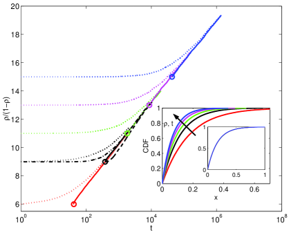
Figure 1: Dynamic evolution of the model for different initializations. Dotted (resp. dash-dotted) lines: starting with the self-similar (resp. uniform) void CDF. Solid (resp. dashed) lines: evolution replotted in terms of an appropriate “initial time” $t_{0}$; notice the collapse of the curves on a straight line, see text. The inset shows void CDFs at different time/density instances (color-coded as in the main Figure); they all collapse upon rescaling to a single CDF (smaller inset).

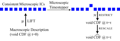
Figure 2: Schematic of coarse dynamic renormalization.

Density provides a cumulative measure of the system evolution (it is the zeroth moment of the particle distribution function). We set out to study in detail the evolution of the void cumulative distribution function, $CDF(x,t)$. This function is defined between $0$ and $1$ in the void size $x$, since at no time do we get voids larger than $1$ (the moment they appear, they get filled). The dotted lines (and the dash-dot line) in Fig. 1 show the evolution of $\delta(t)$ for various initial void distributions (the choice of initial void distributions for these transients will be discussed below). The stochastic simulation uses 100,000 particles; sequential update is used, with a maximum spatial step size of $0.5$. The semilog plot clearly indicates the asymptotic logarithmic regime in time. The inset shows the shape of the void $CDF$ for various simulations and various instances in time, within the logarithmic regime; all shapes when appropriately rescaled with the average void size collapse on a single curve (smaller inset). These two observations (logarithmic time dependence, and collapse of the distributions upon rescaling) clearly suggest the possibility of self-similar evolution dynamics.

In particular, the graph of the time evolution of the densities suggests that $\delta$ becomes eventually proportional to

$$\delta\equiv\frac{1-\rho}{\rho}\sim\frac{1}{A{\rm ln}(t+t_{0})+B}.$$ (2)

Replotting the data in view of the above relation collapses the Fig. 1 curves onto a single line; the role of $t_{0}$ will be discussed below. This implies that the dynamical evolution of $\delta$ eventually follows the differential equation:

$$\frac{d\delta}{dt}\sim-\delta^{2}\exp\left(-\frac{1}{A\delta}\right).$$ (3)

(and hence a similar equation can easily be obtained for $\epsilon$). The dynamics of (3) share the asymptotic behavior of Eq. (1).

We now test the self-similarity hypothesis for the $CDF$ evolution. If the dynamics of the $CDF$ are self-similar and stable, all initial distributions will asymptotically approach the same self-similar shape (modulo rescaling) while they densify and slow down. Our goal is to find the self-similar shape at a convenient scale – a relatively low density, when the evolution dynamics are still fast. Our main assumption is that the void $CDF$ is a good observable for the system dynamics – i.e., that a macroscopic evolution equation (possibly averaged over several experiments) conceptually exists for its dynamics, even though it is not available in closed form. Starting with a given void $CDF_{0}$ with $\delta=\delta_{0}$ we lift to an ensemble of microscopic realizations of it – that is, grain configurations possessing the given void $CDF$. This “lifting” is accomplished here by randomly selecting the voids from $CDF_{0}$ as grains are “put down” on the line; $\delta_{0}$ indirectly selects the scale at which we will perform our computation. We then evolve each of these realizations based on true system stochastic dynamics for a time horizon $\tau$. Finally, we obtain the ensemble averaged void $CDF(x,\tau)$ and its $\delta(\tau)=\delta_{1}$. This is the restriction step of equation-free computation: evaluating the macroscopic observables of detailed, fine scale computations. We now rescale our macroscopic observable (the $CDF(x,\tau)$), using the ensemble average $\delta_{1}$, to the original $\delta_{0}$: $\widehat{CDF}(\delta_{0}x/\delta_{1},\tau)=CDF(x,\tau)$. (Clearly this requires the largest void in the rescaled $\widehat{CDF}$ to be less than $1$ – a condition that one may expect to prevail at high enough densities). We then discard the simulations we performed, and start a new ensemble of simulations at the original density, but with the more “mature” $\widehat{CDF}$. The map from current void $CDF$ to future void $CDF$ is the “coarse timestepper” of the unavailable equation for the macroscopic observable evolution; the composition of this map with the rescaling step constitutes the “renormalized coarse timestepper”, the main tool of our dynamic renormalization procedure, schematically summarized in Fig. 2. Given this map, several approaches to the computation of the long-term coarse self-similar dynamics exist. The simplest is successive substitution – we repeat coarse renormalized time-stepping again and again, and observe the approach of the void $CDF$ to its self-similar shape at the scale we chose (parametrized by $\delta_{0}$). The fixed point of this procedure lies on the group orbit of scale invariance for the $CDF$ dynamics; it was selected through a “pinning” or “template” condition (our choice of $\delta_{0}$). This dynamic renormalization iteration, with $\tau=4$ is shown in Fig. 3a, starting from a uniform void distribution with $\delta_{0}=0.2$; the inset shows the third iteration before (dotted line) and after (solid line) rescaling.

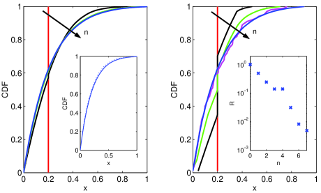
Figure 3: a. Successive evolution of an initially uniform CDF profile with renormalization: the inset shows the profile at the n=3 iteration before (dashed) and after (solid) rescaling. b. Newton-Krylov-GMRES fixed point renormalization calculation, starting from uniform void CDF; the inset shows the decrease of the norm of the residual vector at each Newton step.

Successive substitution will converge to stable self-similar solutions. It is also, however, possible, to use fixed point algorithms to converge to the self-similar void $CDF$ at $\delta_{0}$. In effect, we wish to solve a functional equation for the fixed point of the renormalized timestepper:

$$\widehat{CDF}(x,\tau)-CDF(x,0)=0.$$ (4)

Fixed point algorithms (like Newton’s method) require the repeated solution of systems of linear equations involving the Jacobian matrix of some discretization of Eq. (4). Since we have no closed form equations for the void $CDF$ evolution, this Jacobian is unavailable; yet equation-free methods of iterative linear algebra (like GMRES Kelley_Saad ) allow the solution of the problem through a sequence of matrix-vector product estimations. In our case these estimations are obtained through the “lift-run-restrict-rescale” protocol performed at appropriately selected nearby initial distributions (for details, see Manifesto ). Short bursts of stochastic simulation from nearby initial void distributions allows us to estimate the action of the Jacobian on selected perturbations, and hence the solution of linear equations and ultimately, of the nonlinear fixed point problem. Fig. 3b shows the iterates of such a matrix-free fixed point computation for Eq. (4) through a Newton-Krylov GMRES algorithm applied to a 100-point uniform finite difference discretization of the void $CDF$ in $x$; our initial guess was a uniform void $CDF$ ($\delta_{0}=0.2$), and we converge to the self-similar shape within a few iterations; the inset shows the evolution of the norm of the residual vector with iteration number. Lifting from this coarse description (100 numbers) to realizations of the $CDF$ (200,000 particles) involved linear interpolation of the $CDF$. Relatively short runs ($\tau=1$) were used to construct the coarse renormalized timestepper in Fig. 3b; its fixed point is independent of the reporting horizon $\tau$.

Wrapping traditional numerical algorithms around coarse timesteppers enables several computational tasks, of which the fixed point computation above is only one example. Another interesting example is the so-called coarse projective integration; here, short runs of the stochastic simulation are used to estimate the local time derivatives of the macroscopic observables (e.g. of the void $CDF$); these estimates are used to “project” the void $CDF$ “far” into the future. The simplest such algorithm is projective forward Euler; see Manifesto for multi-step and implicit coarse projective integration. One does not evolve the microscopic problem; one evolves the coarse-grained closure of the microscopic problem, which is postulated to exist, but is not explicitly available. Here we apply coarse projective integration backward in time (as discussed in GearReverse this is appropriate for systems with large time scale separation between fast stable dynamics and slow dynamics). Starting with the self-similar $CDF$ at some (relatively large) density (see Fig. 4 and its insets) we lift to microscopic realizations, evolve briefly forward in time, and estimate the rate of void $CDF$ evolution.

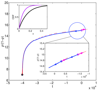
Figure 4: Reverse coarse projective integration: the dotted pink line is the forward estimation of the rate; the solid blue line is the projection backward in time. The upper inset shows (in the same color code as the large dots in the figure) the CDF profile at the beginning and the end of the overall run.

This rate (estimated from the short pink run) is used to project the void $CDF$ for a (longer) interval backward in time (in blue). The forward simulations are then discarded, and new simulations are initialized at the “earlier” void $CDF$. Repeating the procedure clearly shows an acceleration in backward time as the density becomes lower; the probability of large voids becomes increasingly larger, the backward dynamics evolves faster and faster and their fluctuations intensify, making rate estimation from the short forward runs difficult. Fig. 4 seems to suggest a “reverse finite time” rate singularity. This is only a visual suggestion, however; as the density becomes lower, we do not expect an evolution equation for the void CDF to provide a good model. More detailed physical modeling of the void-filling process will be required for the study of this backward dynamics at lower densities to become meaningful.

It is this “visual suggestion” of a backward explosion of the density evolution rate that suggested fitting the data as a function of $t+t_{0}$; we find that, if we initialize with the self-similar $CDF$ (at whatever density), evolution data can be fitted almost perfectly with a straight line for the appropriate $t_{0}$ in Fig. 1. Based on Eq. (2), the value of the term $B$ from all of our trajectories suggests that at time $t+t_{0}=1$ the self-similar $CDF$ density is $\sim 0.60$; that is, $t_{0}-1$ is the time that it takes for a simulation initialized with the self-similar void $CDF$ at density 0.60 to evolve to the initial density of our computational experiments (our $t=0$). When the initial condition is different than the self-similar $CDF$ (e.g. if it is a uniform distribution, see the dash-dot line in Fig. 1) finding a good $t_{0}$ does not collapse the entire transient on a straight line – we see, however, that the solution asymptotically approaches the self-similar one (dashed line).

In summary, in this paper we implemented equation-free, coarse-grained dynamic renormalization (simulation forward and backward in time, as well as fixed point computations) to study the evolution of the void $CDF$ for a model glassy compaction problem; we found this evolution to be governed by apparent asymptotic self-similarity over the range of densities we could reliably compute. The procedure is, in principle, capable of converging to both stable and unstable self similar solutions, find similarity exponents when they exist, as well as to quantify the fixed point stability (by using matrix-free iterative eigensolvers like Arnoldi). In a continuation / bifurcation context the algorithms can be used to track self-similar solutions in parameter space, detect their losses of stability and bifurcations; of particular interest is the onset, in parameter space, of self-similar dynamics, which will appear in our formulation as a fixed point bifurcation template . Finally, coarse projective integration (forward or reverse) can be performed in physical space (void $CDF$ evolution in time) or in renormalized space (renormalized void $CDF$ evolution in logarithmic time). We believe that the bridging of continuum numerical techniques with microscopic simulations we illustrated here may be helpful in the coarse grained study of glassy dynamics through atomistic/stochastic models, especially when the dynamics depend on parameters of the microscopic rules.

Acknowledgments IGK acknowledges the support of a NSF-ITR grant. PGK acknowledges the support of NSF-DMS-0204585, NSF-CAREER and the Eppley Foundation for Research.

References

- (1) P.G. Debenedetti, Metastable Liquids, Concepts and Principles, Princeton Univ. Press (Princeton, 1996); P.G. Debenedetti and F.H. Stillinger, Nature 410, 259 (2001).
- (2) J.B. Knight et al., Phys. Rev. E 51, 3957 (1995); E.R. Nowak et al., Phys. Rev. E 57, 1971 (1998); E.R. Nowak et al., Powder Technol. 94, 79 (1997); see also the review by H.M. Jaeger et al., Rev. Mod. Phys. 68, 1259 (1996); P. Philippe and D. Bideau, Europhys. Lett. 60, 677 (2002).
- (3) G.H. Fredrickson and H.C. Andersen, Phys. Rev. Lett. 53, 1244 (1984) and J. Chem. Phys. 84, 5822 (1985); see also the review by G.H. Fredrickson, Annu. Rev. Phys. Chem. 39, 149 (1988).
- (4) See e.g., P. Sollich and M.R. Evans, Phys. Rev. Lett. 83, 3238 (1999).
- (5) W. Götze and L. Sjögren, Z. Phys. B 65, 415 (1987); E. Leutheusser, Phys. Rev. A 29, 2765 (1984); U. Bengtzelius et al., J. Phys. C. 17, 5915 (1984);
- (6) E. La Nave et al. Phys. Rev. Lett. 88, 225701 (2002); A. Scala et al., Phys. Rev. Lett. 90, 238301 (2003); M. Scott Shell et al., Phys. Rev. Lett. 92, 169902 (2004)
- (7) P. G. Kevrekidis et al., Phys. Lett. A 318 364-372 (2003).
- (8) R. Stinchcombe and M. Depken, Phys. Rev. Lett. 88, 125701 (2002).
- (9) E. Ben-Naim et al., Phys. D 123, 380 (1998).
- (10) D. G. Aronson et al., nlin.AO/0111055; C. Siettos et al., Nonlinearity, 16 497 (2003); C. W. Rowley et al., Nonlinearity 16, 1257 (2003)
- (11) I. G. Kevrekidis et al., Comm. Math. Sciences 1(4) 715 (2003); K. Theodoropoulos et al. Proc. Natl. Acad. Sci. USA 97 9840 (2000); C. W. Gear et al. Comp. Chem. Eng. 26 941 (2002).
- (12) L. Chen et al., J. Non-Newtonian Fluid Mech. 120 215 (2004)
- (13) see e.g. M.J. Landman et al., Phys. Rev. A 38, 3837 (1988); B.J. LeMesurier et al., Phys. 31D, 78 (1986); ibid. 32D, 210 (1988).
- (14) C. T. Kelley, Iterative Methods for Linear and Nonlinear Equations (Frontiers in Applied Mathematics, Vol. 16), SIAM, Philadelphia, 1995; Y. Saad, Iterative methods for sparse linear systems, PWS Publishing CO., Boston, 1995;
- (15) C. W. Gear and I.G. Kevrekidis, Phys. Lett. A 321, 335 (2004). G. Hummer and I.G.Kevrekidis, J. Chem. Phys. 118, 10762 (2003).