Mirages and many-body effects in quantum corrals

Abstract

In the experiment of the quantum mirage, confinement of surface states in an elliptical corral has been used to project the Kondo effect from one focus where a magnetic impurity was placed, to the other empty focus. The signature of the Kondo effect is seen as a Fano antiresonance in scanning tunneling spectroscopy. This experiment combines the many-body physics of the Kondo effect with the subtle effects of confinement. In this work we review the essential physics of the quantum mirage experiment, and present new calculations involving other geometries and more than one impurity in the corral, which should be relevant for other experiments that are being made, and to discern the relative importance of the hybridization of the impurity with surface ($V_{s}$) and bulk ($V_{b}$) states. The intensity of the mirage imposes a lower bound to $V_{s}/V_{b}$ which we estimate. Our emphasis is on the main physical ingredients of the phenomenon and the many-body aspects, like the dependence of the observed differential conductance with geometry, which cannot be calculated with alternative one-body theories. The system is described with an Anderson impurity model solved using complementary approaches: perturbation theory in the Coulomb repulsion $U$, slave bosons in mean field and exact diagonalization plus embedding.

I Introduction

The study of many-body phenomena in nanoscale systems is attracting a lot of attention in recent years. Progress in nanotechnology made it possible to construct nanodevices such as quantum dots (QD’s) which act as ideal one-impurity systems in which the Kondo physics is clearly displayed [1, 2, 3, 4]. The spectral density of localized electrons of a magnetic impurity in a metallic host, described by the impurity Anderson model [5], is known to display a resonance near the Fermi energy in the localized (or Kondo) regime [6]. The conductance through a QD is proportional to this density and calculations of the latter using the Wilson renormalization group leads to a good agreement with experiment [7, 8]. In contrast to the density of localized electrons, the density of conduction electrons coupled to the former shows a dip or Fano antiresonance [9] (see section 3). Using the fact that the tip of the scanning tunneling microscope (STM) captures essentially conduction electrons, Fano line shapes have been observed using scanning tunneling spectroscopy (STS) for different cases of magnetic impurities on metal surfaces [10, 11, 12, 13, 14, 15, 16, 17, 18, 19]. They should also manifest in the conductance through quantum wires side-coupled to QD’s [20, 21, 22, 23, 24, 25]. The impurity Anderson model also describes the physics of the conductance through arrays of QD’s weakly coupled to conducting leads [26].

A quantum corral is an area of about 40 nm² delimited by a closed line of typically several tenths of atoms or molecules placed next to each other one at a time on an atomically flat metallic surface using a STM. The same microscope can be used to perform STS to study with meV resolution the electronic density inside these corrals [12, 27, 28, 29]. Particularly interesting are the (111) surfaces of Cu, Au and Ag. These metals have nearly spherical Fermi surfaces with eight necks at the [111] and equivalent directions in which a gap opens. This allows the presence of Shockley states localized at the (111) surface uncoupled to the bulk states for small wave vector parallel to the surface and with nearly free electron dispersion [30]. STS experiments performed on these surfaces reveal fascinating standing-wave patterns and one can see the density coming from the wave functions obtained solving the Schrödinger equation for a two-dimensional free electron gas inside a hard-wall corral [12, 13, 28, 29, 31]. Experiments in which different atoms or molecules were used to build the corral (Co, Fe, S, CO) suggest that the details of the boundaries are not important for the physics. A continuous description of the boundary is justified by the fact that the Fermi wave length $2\pi/k_{F}\sim 3$ nm is larger than the distance between adatoms. However, as discussed in section 6, the corrals are leaky and the hard-wall assumption should be abandoned for a quantitative description.

The experiment of the quantum mirage is a beautiful combination of the physics of the quantum corral and the many-body Kondo effect. One Co atom acting as a magnetic impurity is placed at the focus of an elliptical corral built on the Cu(111) surface, and a Fano dip is observed not only at the place of the impurity, but remarkably also at the empty focus with reduced magnitude [12]. Variants of this experiment involving other corral shapes and more that one impurity were presented in a conference [13]. In the original experiment, the space dependence of $\Delta dI/dV$, the differential conductance after subtracting the corresponding result without impurity, clearly resembles the density of the state number 42 in increasing order of energy of free electrons in a hard-wall elliptical corral. This suggests that the main features of this space dependence can be explained by a one-body calculation. In fact, important features, like the possibility of obtaining mirages out of the foci can be understood by a simple tight-binding calculation [32] or from Green functions using hard-wall eigenstates [33]. Interesting effects like anti mirages were predicted for a non-magnetic impurity inside a hard-wall elliptical corral [34], and quantum mirages in s-wave superconductors were calculated [35]. Also phenomenological scattering theories in which the energy dependence of the Kondo resonance (directly related with the voltage dependence of $dI/dV$) as well as an inelastic part of the scattering are taken from experiment, are able to describe quantitatively the space dependence [31, 36, 37]. However, the calculation of the line shape of $dI/dV$, its dependence on the particular geometry of the corral, temperature or magnetic field, and the effects of interaction between impurities is out of the scope of these one-body approaches.

The first calculation of the voltage dependence of $dI/dV$ has been done by one of us using perturbation theory in the Coulomb repulsion of the Anderson model $U$ [38, 39] A many-body calculation of the mirage effect is a challenge due to the particular nature of the conduction states brought by the confinement in the corral. In particular, available exact results for thermodynamic properties of the Kondo and Anderson impurities, obtained with the Bethe ansatz, assume a constant density of conduction states [40, 41, 42], while the Wilson renormalization group [43] (which allows accurate calculation of dynamical properties and was used in the context of nanoscopic systems and STS [7, 8, 44, 45, 46]), requires high symmetry around the impurity. If only a finite number of hard-wall eigenstates with well defined energies are mixed with the impurity (a problem that can be treated with exact diagonalization [47, 48]), the line shape of $\Delta dI/dV$ becomes qualitatively wrong (see section 6). The reason is that the separation of the relevant energy levels is large in comparison with the Kondo temperature $T_{K}\sim 53$ K, while one knows that for a well developed Kondo resonance to exist, $T_{K}$ should be larger than the average separation of the relevant levels [49]. This points to the need of including a finite width of the corral eigenstates, which become resonances [38]. This need persists in presence of direct hybridization of the impurity with bulk states as shown in section 6 [50]. The width of the resonances cannot be too large because otherwise the space dependence of the state 42 of the elliptical corral, observed in $dI/dV$ [12] would be blurred.

A subject of current interest and debate in the literature is the relative importance of the hybridization of the impurity with bulk $V_{b}$ and surface $V_{s}$ states. A first principles calculation seems not possible because of the large supercells needed. They should contain more than 10 layers perpendicular to the [111] direction in order for the Shockley surface state to develop, and more than 100 atoms per layer to reach the dilute limit of Co impurities on the surface [54]. On the basis of the rapid decay in $\Delta dI/dV$ as the STM tip is moved away from an impurity on a clean (111) surface, and a jellium theory of Plihal and Gadzuk [55], Knorr et al. concluded that bulk states dominate the formation of the Kondo singlet [17, 18]. This is in agreement with tight-binding calculations [54]. However, recently Lin, Castro Neto and Jones, using a nearly free electron approximation, including the effect of the gaps in the [111] and equivalent directions and calculating the wave functions under an adequate surface potential, concluded that the Kondo effect in the Cu(111) surface is dominated by surface states [56]. They also obtained good agreement with experiment for the distance dependence of the amplitude of $dI/dV$ and its voltage dependence on top of the impurity. Using a similar approach, but without attempting to solve the many-body problem, Merino and Gunnarsson concluded that surface states play an important role in the differential conductance for a system with a magnetic impurity on a clean (111) surface [57]. Therefore, the issue of the relative importance of $V_{b}$ and $V_{s}$ remains unclear. In contrast, in absence of the impurity, the relative contribution of the surface states to the conductance (STM tip-substrate hybridization) is known to be between 1/2 and 2/3 from experiments in which the bias voltage is swept below the bottom of the surface band ($\sim 0.45$ eV below the Fermi energy) [17, 58, 59].

Since from the experiments we know that the presence of the corral strongly affects electronic structure of the surface states, it is clear that the variation of the line shape of $dI/dV$ for different corrals or positions of the impurity inside the corral and its comparison with theory should help to elucidate the relative role of the hybridization of the impurity with surface and bulk states. A stronger sensitivity to the geometry implies a greater participation of the surface states in the formation of the Kondo resonance. Also the interaction between magnetic impurities inside a quantum corral should increase with the relative importance of surface states [47]. Unfortunately only the voltage dependence of $dI/dV$ for a Co atom on a clean Cu(111) surface and on an elliptical corral built on that surface is available for comparison [12]. Using perturbation theory in $U$ both line shapes are qualitatively explained without bulk states [39] (see section 8). However, as we will show, this seems to be a particular case and usually the shape and width of the Fano dip are more sensitive to the geometry.

In this work we discuss the main aspects of the physics of the quantum mirage. The emphasis is on the basic understanding of the phenomenon and its many-body aspects rather than on quantitative fits. The latter would require more detailed knowledge of matrix elements and their wave vector dependence, crystal fields and other details. We extend previous many-body calculations for the space and voltage dependence of $\Delta dI/dV$ to new different situations. This can serve as a basis for comparison with experiment and help to elucidate the relative participation of surface and bulk states in the formation of the Kondo singlet for a Co atom on a Cu(111) surface. We use three different many-body techniques: perturbation theory in $U$ [60, 61], exact diagonalization plus embedding [62, 63, 64] and a slave-boson mean-field approximation (SBMFA) [66, 6, 21, 25, 26]. The former two have already been applied to the quantum mirages [38, 39, 52, 53, 47] but have the disadvantage that they do not reproduce the correct exponential dependence of $T_{K}$ with the coupling constant for large $U/\Delta$, where $\Delta$ is the resonance level width [65]. Therefore, the SBMFA is more appropriate to study the dependence of the width of the resonance on geometry.

The paper is organized as follows. In section 2 we present the impurity Anderson model for either the corral or open surfaces, and discuss its assumptions and limitations. Section 3 discusses the Kondo resonance and Fano antiresonance in the simplest version of the model for later comparison. The formalism and basic equations that determine the tunneling current are presented in section 4, using a many-body formalism, including tunneling of the tip of the STM with surface, bulk and impurity states. Section 5 is rather technical and explains the different many-body approaches. In section 6 we explain the effects of the confinement on the surface states, and how they are transmitted to the Kondo resonance and the line shape of the mirage effect. Section 7 is devoted to the space dependence of the differential conductance $dI/dV$ inside an elliptical quantum corral, the effect of the impurity on it ($\Delta dI/dV$), and the relation of these quantities with the wave functions of the surface states inside the corral. This brings insight into the effect of the width of the surface states and what controls the intensity at the mirage point. In section 8 we present results for the dependence of $\Delta dI/dV$ on bias voltage in different situations: clean surface, elliptical corrals and a circular corral. In section 9 we estimate a lower bound for the participation of surface states in the Kondo resonance. In section 10 the interaction between two Anderson impurities inside an elliptical corral is discussed. Section 11 contains a summary and a discussion.

II The model

In this section, we explain and discuss the model used to describe the electronic structure of a system composed of one magnetic impurity interacting with surface and bulk states. The case of two impurities is left for section 10. The surface states can correspond to eigenstates of a clean perfect surface, or to a surface with a soft-wall corral. In both cases, the energy spectrum of the surface states is continuous. The wave functions $\varphi_{j}(r)$ of the surface eigenstates are normalized in a large area [52, 56]. Of course, all physical results are independent of this area.

We take only one localized $d$ orbital for the impurity. Technically it renders some many-body techniques easier (except the SBMFA). Previously Újsághy et al. [67] assumed a fully degenerate ground state while other recent calculations for impurities on (111) surfaces considered the $d_{3z^{2}-r^{2}}$ orbital more important [56, 57, 68]. Tight binding calculations suggest that Cu(111) surface states hybridize more strongly with the Co $3d_{3z^{2}-r^{2}}$ orbital, while bulk states prefer $3d_{xz}$ and $3d_{yz}$ orbitals [54]. Recent accurate calculations using the Wilson renormalization group indicate that for the expected filling of near one $d$ hole per Co impurity, the Kondo resonance becomes strongly asymmetric in the orbitally degenerate case [46]. Then, one would expect in this case also a strongly asymmetric $\Delta dI/dV$ in contrast to the experimental observations for the (111) surface [12, 17]. We neglect the $s,p$ orbitals of the impurity.

The Hamiltonian can be written as

$$H = \sum_{j\sigma}\varepsilon_{j}^{s}s_{j\sigma}^{\dagger}s_{j\sigma}+\sum_{j\sigma}\varepsilon_{j}^{b}b_{j\sigma}^{\dagger}b_{j\sigma}+E_{d}\sum_{\sigma}d_{\sigma}^{\dagger}d_{\sigma}+Ud_{\uparrow}^{\dagger}d_{\uparrow}d_{\downarrow}^{\dagger}d_{\downarrow}$$ (2)

$$+\sum_{j\sigma}(V_{s}^{j}d_{\sigma}^{\dagger}s_{j\sigma}+\text{H.c.})+\sum_{j\sigma}(V_{b}^{j}d_{\sigma}^{\dagger}b_{j\sigma}+\text{H.c.}).$$

where $s_{j\sigma}^{\dagger}$ ($b_{j\sigma}^{\dagger}$) are creation operators for an electron in the $j^{th}$ surface (bulk) conduction eigenstate in the absence of the impurity, but including the corral if present. The impurity is placed at the two-dimensional position $R_{i}$ on the surface, and we assume that the hybridization of the impurity $d$ orbital with the surface state $j$ is proportional to its normalized wave function at that point $\varphi_{j}(R_{i})$ [33, 38]. Similarly for the bulk states, the hybridization is proportional to some average $\psi_{j}(R_{i})$ of the bulk wave function in the direction normal to the surface, that depends on $R_{i}$:

$$V_{s}^{j}=V_{s}\lambda\varphi_{j}(R_{i}),\text{ }V_{b}^{j}=V_{b}\psi_{j}(R_{i}),$$ (3)

where $V_{s}$, $V_{b}$ are energies representing local hybridizations in a tight-binding model [32, 39] (see next section) and $\lambda=2.38$ Å is the square root of the surface per Cu atom of a Cu(111) surface. We assume also a constant density of bulk states. However, we must warn that recent calculations obtain a significant dependence of the matrix elements with wave vector [56, 57, 68]. This dependence affects the line shape of $dI/dV$. Nevertheless, one expects that the trends in the modifications of the voltage dependence of $dI/dV$ due to the modifications of the geometry remain the same, at least on a qualitative level. This is also suggested by the weak dependence of the results on the cutoff for the surface states $E_{c}$, which should be introduced in any theory of quantum corrals to avoid divergences in the Green’s functions for the surface states. This can be though as an energy dependent hybridization $V_{s}$ which is constant below $E_{c}$ and goes to zero abruptly at $E_{c}$. A linearly decreasing $V_{s}$ has also been used [38]. Increasing $E_{c}$ leads to a weak increase in the width of the resonances and to a more asymmetric line shape, but the main conclusions regarding the mirage effect are not altered.

The many-body part of the Hamiltonian which renders it non-trivial in all cases is the on-site Coulomb repulsion at the impurity site $U$. Another difficulty is the calculation of the surface wave functions $\varphi_{j}(r)$ for soft walls. They have been calculated exactly for a soft circular corral [52, 53] and can be reasonably well approximated for an elliptical corral [52]. We return to this point in section 6. For open structures, the surface Green’s function can be calculated using scattering theory [31]. However, this renders the many-body problem too difficult.

III Simple picture of the Kondo resonance and Fano antiresonance

Before discussing the many-body techniques and the effect of the corral, we want to illustrate some basic features of the Kondo physics, using the simplest case of the Anderson model in which the impurity is hybridized with only one band (either surface or bulk) with constant density of states $\rho_{0}$ and wave vector independent hybridization. The Hamiltonian is given by Eq. (2) eliminating the terms with $s_{j\sigma}$, considering that the $b_{j\sigma}^{\dagger}$ create Bloch waves, ($b_{{\boldmath k}\sigma}^{\dagger}=(1/\sqrt{N})\sum_{l}\exp(-i{\boldmath k}\cdot{\boldmath R}_{l})b_{l\sigma}^{\dagger}$, where $b_{l\sigma}^{\dagger}$ creates an electron at site $l$ with position ${\boldmath R}_{l}$) and taking $V_{b}^{j}=V/\sqrt{N}$ where $N$ is the number of sites. Then, the impurity is hybridized with the band at one site that we call $i$.

The impurity spectral density $\rho_{d\sigma}(\omega)$ of this model has been calculated accurately using Wilson renormalization group [69] and agree qualitatively with those of perturbation theory in $U$ [61]. The results presented in Fig. 1 (a) were obtained using a self-consistent approach [70] based on an interpolation for the self energy of the Green’s function between the expression up to second order perturbation theory in the Coulomb repulsion $U$ [60, 61] and the exact result for $U\rightarrow\infty$. The resonant level width is $\Delta=\pi\rho_{0}V^{2}$. This approximation works well for $U\leq 8\Delta$ [23].

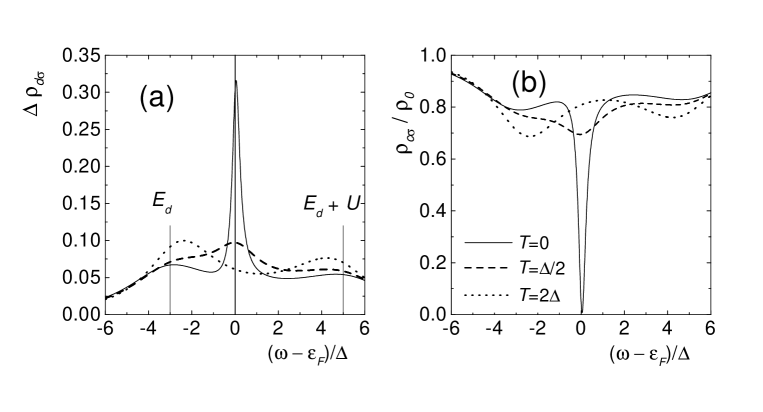
FIG. 1.: (a) spectral density of an impurity hybridized with a featureless conduction band and (b) spectral density at the conduction site hybridized with the impurity, as a function of energy at different temperatures. Parameters are $E_{d}-\epsilon_{F}=-3\Delta$ and $U=8\Delta$.

As seen in Fig. 1 (a), $\rho_{d\sigma}(\omega)$ shows characteristic charge fluctuation peaks (or shoulders for small $U$) at $E_{d}$ and $E_{d}+U$ and another peak near the Fermi energy $\epsilon_{F}$ characteristic of the Kondo regime. This peak is the so called Kondo resonance. Its half width at half maximum corresponds to the Kondo temperature $T_{K}$. At temperatures above $T_{K}$ the Kondo effect disappears and the spectral weight of the Kondo peak is transferred to the other two.

The STS is much more sensitive to the conduction electrons than to the localized ones because the former are more extended in space and reach the tip of the STM with a larger amplitude. The site most affected by the impurity is the one which hybridizes with it ($i$). Using equations of motion (in the same way as done in the next section), it is easy to show that the Green function at this site is (the spin index is dropped for simplicity)

$$G_{ii}(\omega)=G_{ii}^{0}(\omega)+\left[VG_{ii}^{0}(\omega)\right]^{2}G_{d}(\omega),$$ (4)

where $G_{ii}^{0}(\omega)$ is the corresponding Green’s function in the absence of the impurity and $G_{d}(\omega)$ is the Green’s function of the impurity. This equation is exact and does not depend on the approximations for $G_{dd}(\omega)$. If the unperturbed conduction band extends from $-W$ to $W$ then

$$G_{ii}^{0}(\omega)=\sum_{k}\frac{1}{\omega+i\eta-\epsilon_{k}}=\rho_{0}\left[\ln|\frac{W+\omega}{W-\omega}|-i\pi\Theta(W-|\omega|)\right].$$ (5)

If (as usual) $W\gg$ $T_{K}$ and we are interested in energies $|\omega-\epsilon_{F}|\sim T_{K}$, we can neglect the first term inside the brackets and approximate $G_{ii}^{0}(\omega)\cong-i\pi\rho_{0}$. Replacing this in Eq. (4) and using $\rho_{i\sigma}(\omega)=-\mathop{\rm Im}[G_{ii}(\omega)]/\pi$ one obtains the very simple result

$$\frac{\rho_{i\sigma}(\omega)}{\rho_{0}}=1-\pi\rho_{d\sigma}(\omega)\Delta.$$ (6)

Thus a peak in $\rho_{d\sigma}(\omega)$ implies a dip in the conduction density of states and more pronounced near the impurity (see Fig. 1 (b)). In more complex situations, in particular when confinement due to the corral is important, the real part of $G_{ii}^{0}(\omega)$ cannot be neglected and the dip in $\rho_{i\sigma}(\omega)$ is not directly related with the Kondo peak in $\rho_{d\sigma}(\omega)$. In extreme cases, either the dip is replaced by a peak [56] or the structure near $\epsilon_{F}$ disappears, as we will show in section 6.

In any case, the above simple picture corresponds to a first rough approximation of the experimental observations of the voltage dependence of $dI/dV$ for impurities on the (111) surfaces of Cu and noble metals, and we will use it for later comparison.

IV The tunneling conductance

In this section we write the basic equations which relate $dI/dV$ with the Green’s function at the impurity site. We include the hopping of the tip of the STM with the impurity, surface and bulk states in a many-body formalism. The tunneling geometry and energy diagram is shown for example in Fig. 1 of Ref. [31], but the impurity should be included if the tunneling current is measured near it [71], and also the bulk states according to experiment [17, 58, 59].

The total system $S$ consists of a subsystem $S_{H}$ described by the Hamiltonian $H$ [Eq. (2)] and $S_{t}$ contains the tip, which we assume can be described as a non-interacting system with one-particle energies $\epsilon_{k}$ and the Fermi energy set at zero. $S_{H}$ has all one particle energies, including the Fermi level, displaced by $eV$ to lower energies by a bias voltage $V$, where $e$ is the elementary charge. For simplicity we treat the case of positive $V$ in which electrons are transferred from the tip to $S_{H}$. Extension to negative $V$ is trivial using an electron-hole transformation. We assume a local hopping of the tip with the different states

$$H_{mix}=A\sum_{k\sigma}(t_{k\sigma}^{\dagger}h_{\sigma}+\text{H.c.}),$$ (7)

$$h_{\sigma}=\lambda\sum_{j}\varphi_{j}(R_{t})s_{j\sigma}+p\sum_{j}\psi_{j}(R_{t})b_{j\sigma}+q(|R_{t}-R_{i}|)d_{\sigma}.$$ (8)

Here $t_{k\sigma}^{\dagger}$ creates an electron in the tip eigenstate $k$ with spin $\sigma$, $R_{t}$ describes the coordinates of the tip on the plane, and $A$, $p$, and $q$ are parameters that describe the hopping of the tip with the different states of $S_{H}$. The function $q(|R_{t}-R_{i}|)$ is small and decays strongly with the distance between the tip and the impurity $|R_{t}-R_{i}|$ due to the strongly localized nature of the impurity wave function. However, when $R_{t}-R_{i}=0$, a small $q$ introduces an important source of asymmetry in the line shape of $dI/dV$ in addition to that corresponding to the structure of the Green’s functions (see section 8).

Treating $H_{mix}$ in lowest order in perturbation theory and at $T=0$, using Fermi’s golden rule, the current due to the transfer of electrons from $S_{t}$ to $S_{H}$ becomes

$$I=\frac{2\pi e}{\hbar}A^{2}\sum_{\nu}|\langle\nu|\sum_{k\sigma}h_{\sigma}^{\dagger}t_{k\sigma}|g\rangle|^{2}\delta(E_{\nu}-E_{g}-eV),$$ (9)

where $|\nu\rangle$, $E_{\nu}$ are the eigenstates and energies of $S$ and $|g\rangle$ is the ground state assumed non degenerate. Using the same notation with a subscript $H$ for $S_{H}$, we have $|g\rangle=\prod_{k\sigma}t_{k\sigma}^{\dagger}|g_{H}\rangle$ with the product restricted to $k$ such that $\epsilon_{k}<\epsilon_{F}=0$. Replacing above and doing the calculations within $S_{t}$ one has

$$I=\frac{2\pi e}{\hbar}A^{2}\sum_{\nu_{H}}\sum_{k\sigma}^{\prime}|\langle\nu_{H}|h_{\sigma}^{\dagger}|g_{H}\rangle|^{2}\delta(E_{\nu_{H}}-\epsilon_{k}-E_{g_{H}}-eV).$$ (10)

Using the Lehman representation [72], the sum over $\nu_{H}$ is seen to represent the part of the spectral density $\rho_{h\sigma}(\epsilon_{k}+eV)$ of $h_{\sigma}^{\dagger}$ for electron addition. This corresponds to excitations above $\epsilon_{F}$ with positive argument of $\rho_{h\sigma}$ [73]. By symmetry it is independent of $\sigma$. Transforming the sum over the tip states $k$ as an integral assuming a constant density of states $\rho_{t}$ one gets

$$I\left(\frac{4\pi e}{\hbar}A^{2}\rho_{t}\right)^{-1}=\int_{-eV}^{0}\rho_{h\sigma}(\epsilon+eV)d\epsilon=\int_{0}^{eV}\rho_{h\sigma}(\omega)d\omega\text{.}$$ (11)

From here, it is clear that the differential conductance is proportional to the spectral density of the state $h_{\sigma}(R_{t})$:

$$dI/dV\sim\rho_{h\sigma}(eV)=-\frac{1}{\pi}\mathop{\rm Im}G_{h\sigma}(eV),$$ (12)

where $G_{h\sigma}(\omega)=\langle\langle h_{\sigma};h_{\sigma}^{\dagger}\rangle\rangle_{\omega}$ is the Green’s function of $h_{\sigma}(R_{t})$. Therefore, in the rest of the paper we will be mainly concerned on the space and energy dependence of $\rho_{h\sigma}$. This spectral density can be related with the Green’s function for the $d$ electrons $G_{d\sigma}(\omega)=\langle\langle d_{\sigma};d_{\sigma}^{\dagger}\rangle\rangle_{\omega}$, and the unperturbed Green’s functions for conduction electrons using equations of motion. Writing $c_{j\sigma}$ to represent either $s_{j\sigma}$ or $b_{j\sigma}$, the relevant equations can be written in the form

$$(\omega-\epsilon_{j}^{c^{\prime}})\langle\langle c_{j\sigma}^{\prime};c_{j\prime\sigma}^{\dagger}\rangle\rangle_{\omega} = \delta_{jj\prime}\delta_{cc\prime}+\bar{V}_{c^{\prime}}^{j}\langle\langle d_{\sigma};c_{j\prime\sigma}^{\dagger}\rangle\rangle_{\omega},$$ (13)

$$(\omega-\epsilon_{j}^{c})\langle\langle c_{j\sigma};d_{\sigma}^{\dagger}\rangle\rangle_{\omega} = \bar{V}_{c}^{j}\langle\langle d_{\sigma};d_{\sigma}^{\dagger}\rangle\rangle_{\omega},$$ (14)

$$(\omega-\epsilon_{j}^{c})\langle\langle d_{\sigma};c_{j\sigma}^{\dagger}\rangle\rangle_{\omega} = V_{c}^{j}\langle\langle d_{\sigma};d_{\sigma}^{\dagger}\rangle\rangle_{\omega}.$$ (15)

Dropping the spin indices, using these equations and introducing the non-interacting Green’s functions (in absence of the impurity) for conduction electrons

$$G_{s}^{0}(R_{1},R_{2},\omega) = \langle\langle\sum_{j}\varphi_{j}(R_{1})s_{j\sigma};\overline{\varphi}_{j^{\prime}}(R_{2})s_{j\prime\sigma}^{\dagger}\rangle\rangle_{\omega}=\sum_{j}\frac{\varphi_{j}(R_{1})\overline{\varphi}_{j}(R_{2})}{\omega-\epsilon_{j}^{s}},$$ (16)

$$G_{b}^{0}(R_{1},R_{2},\omega) = \sum_{j}\frac{\psi_{j}(R_{1})\overline{\psi}_{j}(R_{2})}{\omega-\epsilon_{j}^{b}},$$ (17)

the Green’s function for the $h$ operators becomes

$$G_{h}(R_{t},R_{i},\omega) = \lambda^{2}G_{s}^{0}(R_{t},R_{t},\omega)+p^{2}G_{b}^{0}(R_{t},R_{t},\omega)+\Delta G_{h}(R_{t},R_{i},\omega),$$ (18)

$$\Delta G_{h}(R_{t},R_{i},\omega) = F(R_{t},R_{i},\omega)F(R_{i},R_{t},\omega)G_{d}(\omega),$$ (19)

$$F(R_{1},R_{2},\omega) = V_{s}\lambda^{2}G_{s}^{0}(R_{1},R_{2},\omega)+pV_{b}G_{b}^{0}(R_{1},R_{2},\omega)+q(|R_{1}-R_{2}|).$$ (20)

Here, the first two terms when replaced in Eq. (12) describe $dI/dV$ in the absence of the impurity, while $\Delta G_{h}$ describes the effect of the impurity on the differential conductance $\Delta dI/dV$.

Note that the space dependence of $dI/dV$ is determined only by the non-interacting conduction electron Green’s functions. In particular at a distance of the impurity larger than $\sim$0.5 nm, $q(|R_{t}-R_{i}|)$ becomes irrelevant, the bulk part becomes less important in $\Delta dI/dV$ due to its more rapid decay with the distance between the tip and the impurity $|R_{t}-R_{i}|$ [74], and the space dependence is dominated by $G_{s}^{0}(R_{t},R_{i},\omega)$. The impurity Green’s function $G_{d}$ can only alter the relative weight of the real and imaginary part of the other factors in $\Delta G_{h}$. There is a natural length scale in the Kondo problem $\xi=\hbar v_{F}/T_{K}$, where $v_{F}$ is the Fermi velocity. It has been interpreted as the size of the cloud of conduction electrons that screen the localized spin in the Kondo effect. The existence of this cloud is still controversial [75, 76, 77]. Theoretical work has shown that the persistent current as a function of flux $j(\Phi)$ in mesoscopic rings with quantum dots changes its shape smoothly as the length of the ring $L$ goes through $\xi$ and that $jL$ is a universal function of $L/\xi$ [78, 79]. However, in our case, it is clear that $\xi$ plays no role in the space dependence of $dI/dV$.

V The many-body techniques

The core of the many-body problem is to solve the impurity Green’s function $G_{d\sigma}$ which enters Eq. (20) and determines $dI/dV$ through Eq. (12). Here we present results using three different techniques: a) perturbation theory up to second order in $U$, b) slave-boson mean-field approximation (SBMFA) and c) exact diagonalization plus embedding (EDE). The first one has been already used by us to study the mirage effect [38, 39, 52, 53] and by one of us [39] and Shimada et al. [80] to study the line shape of $dI/dV$ in absence of the corral. The latter problem was also studied recently using the SBMFA [56], and to the best of our knowledge the results presented in section 8 are the first application of this technique to the mirage effect. EDE has been used in Ref. [47].

A Perturbation theory in the Coulomb repulsion

The starting point is the calculation of the non-interacting problem ($U=0$) but with $E_{d}$ replaced by effective one-particle $d$ level $E_{d\sigma}^{eff}$. Using equations of motion similar to Eqs. (15), and assuming $V_{b}^{2}G_{b}^{0}(R_{i},R_{i},\omega)=-i\delta_{b}$ independent of $\omega$ (as in the simple case of section 3), the resulting non-interacting impurity Green’s function becomes:

$$G_{d\sigma}^{0}(\omega)=\frac{1}{\omega-E_{d\sigma}^{eff}+i\delta_{b}-(V_{s}\lambda)^{2}G_{s}^{0}(R_{i},R_{i},\omega)}.$$ (21)

The first choice for $E_{d\sigma}^{eff}$ would be the Hartree-Fock value $E_{d\sigma 0}^{eff}=E_{d}+U\langle d_{\bar{\sigma}}^{\dagger}d_{\bar{\sigma}}\rangle$ [61]. However, out of the symmetric case $E_{d}+U/2=\epsilon_{F}$, better results are obtained if $E_{d\sigma}^{eff}$ and $\langle d_{\sigma}^{\dagger}d_{\sigma}\rangle$ are calculated self-consistently using interpolative schemes that reproduce correctly the physics not only for small $U$ but also for infinite $U$ [23, 70, 79, 81]. For example, the persistent current in small rings with quantum dots practically coincides with exact results for $U\sim 6\Delta$, where $\Delta$ is the resonant level width [79]. At the symmetric case the theory is quantitatively correct up to $U\sim 8\Delta$ [82]. To avoid self-consistency we take parameters near the symmetric case, for which $E_{d\sigma}^{eff}$ is near the Fermi energy $\epsilon_{F}$. This is consistent with first-principle calculations [83].

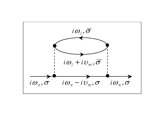
FIG. 2.: Feynman diagram for the contribution to the self energy of the $d$ electrons in second order in the Coulomb repulsion $U$.

The interacting impurity Green’s function can be written in the form

$$G_{d\sigma}^{-1}(\omega)=\left[G_{d\sigma}^{0}(\omega)\right]^{-1}+E_{d\sigma}^{eff}-E_{d\sigma 0}^{eff}-\Sigma_{\sigma}(\omega),$$ (22)

and the approximation consists in calculating $\Sigma_{\sigma}(\omega)$ in second-order perturbation theory in $U$ [60, 61] (the first-order terms are already included in $E_{d\sigma 0}^{eff}$). The corresponding Feynman diagram is shown in Fig. 2. Using the analytical extension of the time ordered $G_{d\sigma}^{0}(\omega)$ to Matsubara frequencies, the expression for the self energy reads

$$\Sigma_{\sigma}(i\omega_{n},T) = U^{2}T\sum_{m}G_{d\sigma}^{0}(i\omega_{n}-i\nu_{m})\chi(i\nu_{m})\text{;}$$ (23)

$$\chi(i\nu_{m}) = -T\sum_{l}G_{d\bar{\sigma}}^{0}(i\omega_{l})G_{d\bar{\sigma}}^{0}(i\omega_{l}+i\nu_{m}),$$ (24)

where the $\omega_{i}$ ($\nu_{m}$) are fermionic (bosonic) frequencies. The evaluation of the Matsubara sums is greatly facilitated by the fact that the unperturbed Green’s function for surface states $G_{s}^{0}(R_{1},R_{2},\omega)$, which for a soft corral involve a continuous distribution of energy, can be well approximated by a sum over a finite number of simple fractions with simple poles in the complex plane [see Eq. (41) of section 6] [52].

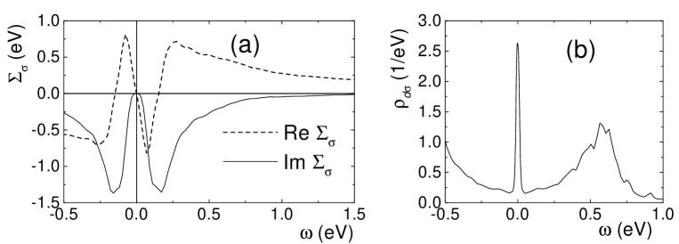
FIG. 3.: (a) Self energy and (b) impurity spectral density as a function of energy for a system with an impurity placed at position $(-0.4a,0)$ inside an elliptical quantum corral with eccentricity 1/2 and size such that the state 35 is at the Fermi level. Parameters are in the text (section 5 A).

In Fig. 3 (a) we show the resulting $\Sigma_{\sigma}(\omega)$ at zero temperature for an elliptical corral with eccentricity $e=1/2$, like that used in the experiment of Manoharan et al. [12], but with semimajor axis reduced to $a=6.46$ nm so that the state 35 of the hard-wall corral falls at the Fermi level. The impurity was placed at a maximum of the wave function of this state ($x=\pm 0.4a$, $y=0$, see Fig. 10). For simplicity we took $V_{b}=0$, and $G_{s}^{0}(R_{1},R_{2},\omega)$ was constructed from hard-wall eigenstates broadened by an imaginary part $\delta=20$ meV [Eq. (41) ]. For the hybridization with surface states we took an energy dependent decreasing function $V_{s}(\epsilon)=0.67$eV$\max\left(1+\frac{\epsilon_{F}-\epsilon}{\text{eV}},0\right)$ [38], which leads to a more symmetric impurity density of states $\rho_{d\sigma}(\omega)$. The zero of energy is set at $\epsilon_{F}=0$, and $E_{d\sigma}^{eff}=22$ meV. We took $U=1$ eV. While $U=2.84$ eV has been estimated [67], this approximation ceases to be reliable for larger values of $U$ [84]. The imaginary part of $\Sigma_{\sigma}(\omega)$ vanishes at $\epsilon_{F}$ and has a quadratic dependence on energy near $\epsilon_{F}$ , respecting Fermi liquid properties [85].

The particular structure of $\Sigma_{\sigma}(\omega)$ near $\epsilon_{F}$ leads to the development of the Kondo peak in the impurity spectral density $\rho_{d\sigma}(\omega)=-\frac{1}{\pi}{\rm Im}G_{d\sigma}(\omega)$. This function is shown in Fig. 3 (b) for a range of energies extending between the bottom of the surface band and the smooth cutoff in the hybridization. The overall structure is similar to that shown in Fig. 1 (a), with two charge fluctuation peaks and the Kondo peak. However, the uneven structure of the conduction band, which in this case is a sum of broadened peaks rather than a flat band, introduces some wiggles. This is particularly clear for the charge fluctuation peak near $E_{d}+U$ $\sim 0.5$ eV. The effects of the confinement will be discussed in the next section.

Unless otherwise indicated, the results presented in this paper were obtained by this technique.

B The slave-boson mean field approximation (SBMFA)

This approximation for the $U\rightarrow\infty$ limit of the Anderson model is in some sense a complement of the previous one, which is valid for small or moderate $U$ [84]. The slave-boson representation consists in writing $d_{\sigma}^{\dagger}=f_{\sigma}^{\dagger}b$ as a product of a fermion operator $f_{\sigma}^{\dagger}$ and a bosonic one $b$ [66]. For $U\rightarrow\infty$, double occupancy is forbidden and this is expressed by the constraint $b^{\dagger}b+\sum_{\sigma}f_{\sigma}^{\dagger}f_{\sigma}=1$ introduced by a Lagrange multiplier $\Lambda$ in the Hamiltonian $H$ [66, 86]. We present the formalism for the $SU(N)$ generalization of our model, in which the index $\sigma$ can run over a set of $N$ degenerate states (instead of only 2). In mean field, the bosonic operators are replaced by a number $b\rightarrow\langle b\rangle=\langle b^{\dagger}\rangle=r$, and $r$ and $\Lambda$ are obtained minimizing the free energy of the resulting model for free fermions. In this approximation, the charge fluctuation peaks (at $E_{d}$ and $E_{d}+U$) are absent in the spectral density. However, in the Kondo regime, for zero or small temperature and energies near the Fermi energy, the approximation seems to be reliable [6]. We restrict our calculations to $T=0$.

In the SBMFA, the impurity Green’s function near the Fermi energy $\epsilon_{F}=0$ is just

$$G_{d\sigma}(\omega)=r^{2}G_{f\sigma}(\omega),$$ (25)

and the Green’s function $G_{f\sigma}(\omega)=\langle\langle f_{\sigma};f_{\sigma}^{\dagger}\rangle\rangle_{\omega}$ is obtained solving the following effective Hamiltonian, which results from Eq. (2) with the above explained replacements

$$H_{eff} = \sum_{j\sigma}\varepsilon_{j}^{s}s_{j\sigma}^{\dagger}s_{j\sigma}+\sum_{j\sigma}\varepsilon_{j}^{b}b_{j\sigma}^{\dagger}b_{j\sigma}+(E_{d}+\Lambda)\sum_{\sigma}f_{\sigma}^{\dagger}f_{\sigma}+\Lambda(r^{2}-1)$$ (27)

$$+r\left[\sum_{j\sigma}(V_{s}^{j}f_{\sigma}^{\dagger}s_{j\sigma}+\text{H.c.})+\sum_{j\sigma}(V_{b}^{j}f_{\sigma}^{\dagger}b_{j\sigma}+\text{H.c.})\right].$$

Minimization of the energy $\langle H_{eff}\rangle$ with respect to $\Lambda$ leads to

$$r^{2}=1-\sum_{\sigma}n_{\sigma}=1-Nn_{\sigma},$$ (28)

where in the second equality we assume $SU(N)$ invariance and

$$n_{\sigma}=\langle f_{\sigma}^{\dagger}f_{\sigma}\rangle=-\frac{1}{\pi}\int d\omega f(\omega){\rm Im}G_{f\sigma}(\omega),$$ (29)

where $f(\omega)$ is the Fermi function.

Using the Hellmann-Feynman theorem [87], the other equation to be solved self-consistently reads

$$\frac{1}{2r}\frac{\partial\langle H_{eff}\rangle}{\partial r}=\Lambda+S+B=0,$$ (30)

$$S=\frac{1}{2r}\sum_{j\sigma}\langle V_{s}^{j}f_{\sigma}^{\dagger}s_{j\sigma}+\text{H.c.}\rangle,\text{ }B=\frac{1}{2r}\sum_{j\sigma}\langle V_{b}^{j}f_{\sigma}^{\dagger}b_{j\sigma}+\text{H.c.}\rangle.$$ (31)

The expectation values entering this equation can be evaluated as integrals over $f(\omega)$ times the imaginary part of Green’s functions of the same form of the first member of the second and third of the Eqs. (15) [88]. From the differences between $H$ (Eq. (2)) and $H_{eff}$ (Eq. (27)) one sees that these equations can be used with $d_{\sigma}$ replaced by $f_{\sigma}$ and a factor $r$ multiplying $V_{s}^{j}$ and $V_{b}^{j}$. Then

$$S=-\frac{1}{\pi}{\rm Im}\left[\int d\omega f(\omega)\sum_{j\sigma}\frac{|V_{s}^{j}|^{2}}{\omega+i\eta-\epsilon_{j}^{s}}G_{f\sigma}(\omega)\right]=-\frac{N}{\pi}V_{s}^{2}\lambda^{2}{\rm Im}\left[\int d\omega f(\omega)G_{s}^{0}(R_{i},R_{i},\omega)G_{f\sigma}(\omega)\right],$$ (32)

where for the last equality we used Eqs. (3) and (17). In a similar way one has

$$B=-\frac{N}{\pi}V_{b}^{2}\mathop{\rm Im}\left[\int d\omega f(\omega)G_{b}^{0}(R_{i},R_{i},\omega)G_{f\sigma}(\omega)\right],$$ (33)

while the $f$ electron Green’s function is:

$$G_{f\sigma}(\omega)=\frac{1}{\omega-E_{d}-\Lambda-(rV_{s}\lambda)^{2}G_{s}^{0}(R_{i},R_{i},\omega)-(rV_{b})^{2}G_{b}^{0}(R_{i},R_{i},\omega)}.$$ (34)

From the self-consistent solution of Eqs. (28) to (34) we obtain $G_{f\sigma}(\omega)$ and $r$. The differential conductance is then obtained using Eqs. (12), (20) and (25). For the calculations shown here, we take $N=2$ because otherwise the line shape becomes too asymmetric in comparison with experiments for the expected 3d⁹ configuration of the Co impurity [46].

In the absence of the corral, for an impurity on a clean surface, we assume constant symmetric density of states as in Eq. (5):

$$\lambda^{2}G_{s}^{0}(R_{i},R_{i},\omega)=\rho_{s}\left[\ln\left(\frac{W_{s}+\omega}{\omega-W_{s}}\right)\right],\text{ }G_{b}^{0}(R_{i},R_{i},\omega)=\rho_{b}\left[\ln\left(\frac{W_{b}+\omega}{\omega-W_{b}}\right)\right]$$ (35)

The self-consistent equations are rather easy to solve for this case and allows us modify the parameters to fit the observed line shape. In Fig. 4 we compare the analytical expression used by Knorr et al. [17] to fit the low energy part of $dI/dV$ and our results within the SBMFA. The same set of parameters is used in section 8 to study the modifications of the line shape in a circular corral. For the bulk density of states we take $\rho_{b}=0.145/$eV per site and spin from its value at the Fermi energy reported by first-principles calculations [89]. $W_{b}$ is determined from the filling of one electron per site $2W_{b}\rho_{b}=1$. From the effective mass $m_{e}^{*}=0.38\ m_{e}$, where $m_{e}$ is the electron mass [28, 90] and a parabolic dispersion, one gets $\rho_{s}=0.045/$eV per site and spin. From the bottom of the surface band we take $W_{s}=0.4$ eV, and we assume for simplicity the same value for the high energy cutoff. As mentioned before, the results are only weakly sensitive to the cutoff. $E_{d}=-0.8$ eV is taken from Ref. [67]. The ratio $V_{b}/V_{s}$ is determined by imposing a fixed ratio of the resonant level due to bulk ($\delta_{b}=\pi\rho_{b}V_{b}^{2}$) or surface ($\delta_{s}=\pi\rho_{s}V_{s}^{2}$) states: a) $\delta_{b}=\delta_{s}$, b) $\delta_{b}=3\delta_{s}$. The magnitude of the hybridization controls the width of the line shape and is a fitting parameter. The value of $p$ in Eq. (8) is fixed in such a way that for a clean surface, near 1/2 of the intensity of $dI/dV$ is due to bulk states [17, 58, 59]. Therefore we took $p=1/3$ to compensate the approximate ratio $\rho_{b}/\rho_{s}\simeq 3$. Instead $q$ is used as a fitting parameter which controls the asymmetry in $dI/dV$. In addition, for the fit of Fig. 4, we shifted the minimum of $dI/dV$ and used a factor that represents the quantity $\frac{4\pi e}{\hbar}A^{2}\rho_{t}$ in Eq. (11). From the fitting procedure we obtain a) $q=0.04$, $V_{s}=0.895$ eV and $V_{b}=0.499$ eV, b) $q=0.035$, $V_{s}=0.604$ eV and $V_{b}=0.583$ eV.

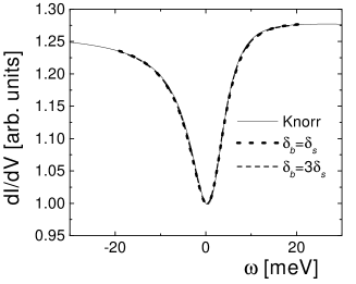
FIG. 4.: Comparison between the analytical expression used in Ref. 17 to fit the low energy part of $dI/dV$ and our results within the SBMFA. The parameters are explained in section 5 B.

C Exact diagonalization plus embedding (EDE)

This method developed for impurity problems [62, 63], consists in solving numerically by the Lanczos method part of the system $H_{0}$ which contains a finite number of relevant many-body states, and treating a one-body term $H^{\prime}$ which connects it to the rest of the non interacting system $H_{r}$, by an approximate method. For example, $H=H_{0}+$ $H^{\prime}+$ $H_{r}$ can describe a quantum wire with an embedded quantum dot modeled by the impurity Anderson model in a chain [22, 24, 64]. In this case $H_{0}$ contains the dot and a few adjacent sites, and $H^{\prime}$ is the hopping of the extreme sites included in $H_{0}$ to their nearest neighbors in $H_{r}$. For an impurity in a quantum corral, $H_{0}$ should contain the impurity and a few conduction eigenstates of the hard wall corral, which acquire a finite width $\delta$ due to hopping to the rest of the system [47]. As we show in the next section, this width is essential to describe the physics.

The method starts by solving the one-particle Green’s functions for $H^{\prime}=0$. Those for $H_{r}$ are known, and those of $H_{0}$ are calculated using the recursion technique combined with the Lanczos method. Off diagonal matrix elements are calculated from diagonal elements of hybrid states, involving sum and difference of basis states. This information is gathered in a matrix ${\bf g}$. For a non-interacting system ($U=0$), the Green’s function of $H$, which we denote by ${\bf G}$, can be calculated from the Dyson equation ${\bf G=g+gH^{\prime}G}$. This is taken as an approximation for the interacting system. Obviously the approximation is exact for $H^{\prime}=0$ and any value of the interaction, and also in the non-interacting case.

This approximation should be used with caution and incorrect results can be obtained if it is applied outside its range of validity. For the Anderson model, a reasonable criterion is that the size of the exactly solved part should be smaller or of the order of the characteristic length $\xi\sim\hbar v_{F}/T_{K}$ mentioned in section 4 [22, 24, 64]. In practice, even when $\xi$ is ten times larger than the size of the system, the resulting value of the impurity spectral density at the Fermi energy $\rho_{d\sigma}(\epsilon_{F})$ practically coincides with the exact value, known from Friedel’s sum rule [22, 64] For much larger $\xi$, the approximation is not valid. For example, the width of the Kondo resonance near the symmetric case $E_{d}+U/2\sim\epsilon_{F}$ behaves as $U^{-2}$ [64], what is incorrect for large $U$ (implying small $T_{K}$ and large $\xi$) [65]. In the mirage experiment, using the velocity of bulk states $v_{F}=1.57\times 10^{8}$ cm/s, then $\xi\sim 200$ nm and the size of the ellipse is $2a\sim 14$ nm.

This technique is easier to implement than others for the case of more than one impurity in the quantum corral and will be used in section 10.

VI The role of confinement

A One-body effects

In the experiments of the mirage effect in an elliptical corral with eccentricity $e=1/2$ and semimajor axis $a=7.13$ nm, the space dependence of $\Delta dI/dV$ reminds the wave function of the state number 42 for a two-dimensional free electron gas in a hard-wall corral [12]. This already points out the importance of the confinement in the problem. Although the hard wall is not a realistic assumption, some basic features of the mirage effect can be understood with it [32, 33]. The eigenstates which determine the surface Green’s function Eq. (17) have in general a continuous distribution in energy, but the spectrum is discrete for a hard-wall corral. From the form of the Schrödinger equation we know that for corrals of the same size, the separation between any two energy levels is inversely proportional to the area of the corral [52]. Therefore in principle changing the size of the corral allows to single out one energy level at will, place it near the Fermi energy $\epsilon_{F}$, and observe it by STS, since as explained in section 4, it essentially captures the conduction states near $\epsilon_{F}$. While this is a good starting point for the understanding of the phenomenon, due to the soft character of the walls, the corral eigenstates become resonances and there is a delicate interplay between the width of these resonances and the separation between energy levels.

While in presence of soft walls the surface eigenstates form a continuum, it turns out very useful not only for the understanding of the physics but for the practical implementation of the many-body techniques, that under general assumptions, the surface Green’s function can be written as a discrete sum of contributions from resonances [51]. We have shown this explicitly for the case of a circular confining potential of the form

$$V(r,\theta)=V_{\text{conf}}\frac{\hbar^{2}}{2m_{e}^{*}r_{0}^{2}}\delta(\frac{r}{r_{0}}-1),$$ (36)

where $r,\theta$ are the polar coordinates on the plane and $V_{\text{conf}}$ is a dimensionless constant controlling the strength of the confinement potential [52, 53]. The result is

$$G_{s}^{0}(r,\theta,r^{\prime},\theta^{\prime},\omega)=\sum_{n,m}\frac{C_{n}^{m}\ J_{m}(k_{n}^{m}r)J_{m}(k_{n}^{m}r^{\prime})\ e^{im(\theta-\theta^{\prime})}}{\omega-\epsilon_{n}^{m}+i\delta_{n}^{m}}.$$ (37)

The complex poles $\epsilon_{n}^{m}-i\delta_{n}^{m}=(\hbar k_{n}^{m})^{2}/(2m_{e}^{*})$, where the complex wave vectors $k_{n}^{m}$ are the zeros of a function $F_{m}(k)$ explained below which lead to positive $\delta_{n}^{m}$. The coefficients $C_{n}^{m}\$are

$$C_{n}^{m}=-\frac{i\ k_{n}^{m}}{\frac{\partial(F_{m}(k))}{\partial k}|_{k=k_{n}^{m}}}.$$ (38)

$F_{m}(k)$ is a function of the Bessel functions of the first ($J_{m}$) and second ($Y_{m}$) kind which is related to the normalization of the wave functions in the continuum. Its expression is

$$F_{m}(k) = A_{m}^{2}(k)+B_{m}^{2}(k)\text{, with }A_{m}(k)=1+\frac{V_{\text{conf}}(kr_{0})^{-1}}{\frac{Y_{m+1}(kr_{0})}{Y_{m}(kr_{0})}-\frac{J_{m+1}(kr_{0})}{J_{m}(kr_{0})}},$$ (39)

$$B_{m}(k) = \left(1-A_{m}(k)\right)\frac{J_{m}(kr_{0})}{Y_{m}(kr_{0})}.$$ (40)

In practice, in Eq.(37) one includes only the terms for which $\epsilon_{n}^{m}<E_{c}$, where the cutoff energy $E_{c}$ is of the order of 1 eV.

The results of Ref. [52] suggest that for corrals of other shapes and not too weak confinements, one can approximate the surface Green’s function as

$$G_{s}^{0}(R_{1},R_{2},\omega)\simeq\sum_{j}\frac{\varphi_{j}^{c}(R_{1})\overline{\varphi}_{j}^{c}(R_{2})}{\omega-\epsilon_{j}+i\delta_{j}},$$ (41)

where $\varphi_{j}^{c}(R)$ are the discrete eigenstates of the hard wall corral and $\epsilon_{j}$ are their energies, calculated with a slightly renormalized effective mass $m_{e}^{*}$ (increased by about 10% [52]), and $\delta_{j}$ are the width of the resonances, which to a very good approximation are linear in energy $\delta_{j}=\delta_{F}(\epsilon_{j}-\epsilon_{b})/(\epsilon_{F}-\epsilon_{b})$, where $\delta_{F}$ is the width of the resonance at the Fermi level and $\epsilon_{b}$ is the bottom of the surface band [52]. As we show below, this width plays an essential role in the many-body results. In some cases, for simplicity and since it does not affect much the results, we will take constant $\delta_{j}=\delta_{F}$.

B Many-body effects

Usually, as in the simple case of section 3, the Anderson impurity is hybridized with a continuous band of conduction states, flat on the scale of $T_{K}$. However, if one takes $V_{b}=0$ and a hard-wall assumption for the surface states, the Anderson impurity in our model is mixed with a discrete set of conduction states with a significant separation between adjacent levels. Does a Kondo resonance form in this case? This question has been addressed in the context of mesoscopic systems [49]. We illustrate it with a simple problem of a ring of $L$ sites described by a tight binding model with hopping $t$, in which one particular site has on-site energy $E_{d}=-t$, a Coulomb repulsion $U=2t$ and hopping $0.4t$ with their nearest neighbors [79]. We take half filling, what implies $\epsilon_{F}=0$ and assume that the ring is threaded by half a flux quantum in order to have (as in the case of the quantum mirage) an important hybridization of a conduction state at the Fermi energy $\epsilon_{F}$ with the impurity. This is a symmetric Anderson model with a discrete spectrum of conduction states. The impurity spectral density $\rho_{d\sigma}(\omega)$ calculated with perturbation theory in $U$ is shown in Fig. 5. For $L=800,$ the average separation between the levels which hybridize with the impurity $d=8t/L$ is an order of magnitude smaller than the half width of the resonance $T_{K}\sim 0.1t$ and we can see a structure similar to Fig. 1 (a). In particular, the Kondo resonance at $\epsilon_{F}$ can be visualized. For $L=80$ one has $d\sim T_{K}$ and the spectral function has some similarities with that of the continuous conduction band, but with an important internal structure. For $L=8$, for which $d\sim 10T_{K}$, the central Kondo peak is absent [91].

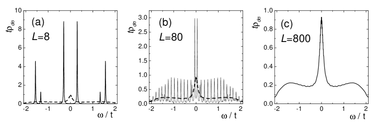
FIG. 5.: Impurity spectral density as a function of energy for a ring of $L$ sites described by the impurity Anderson model and several values of $L$. An artificial broadening $\eta=0.01t$ was introduced for each peak. The result for $L=800$ is also shown with a dashed line in (a) and (b) to facilitate comparison. Parameters in the text (section 6 B).

As we see, to obtain a well defined Kondo resonance with discrete conduction states, it is necessary that $d\lesssim T_{K}$. Instead, in the mirage experiments one has $d\gg T_{K}$. While $T_{K}\sim 5$ meV [12], the average distance between the energy levels that have an important hybridization with the impurity (those shown in Fig. 10) is of the order of 100 meV. This shows the need to take into account the finite width $\delta_{j}$ to the conduction states. The evolution with $\delta_{j}$ (taken for simplicity independent of $j$) of $\rho_{d\sigma}(\omega)$ and the change in the surface part of the conduction density of states after addition of the impurity $\Delta\rho_{s\sigma}(\omega)$ for the elliptical corral with $e=1/2$ studied experimentally [12] is shown in Fig. 6. The impurity is placed at one focus of the ellipse. $\rho_{s\sigma}(\omega)$ is given by Eqs. (8) , (12) and (20) with $p=q=0.$ As anticipated above, for very small $\delta$, the impurity spectral density does not show a well defined resonance at $\epsilon_{F}$. As a consequence, there is a marked disagreement of $\Delta\rho_{s\sigma}(\omega)$ with the observed $\Delta dI/dV$ (which is very similar to the bottom left curve). For $\delta=1$ meV, $\rho_{s\sigma}(\omega)$ has two peaks (instead of antiresonances as in section 3) at the same positions of $\rho_{d\sigma}(\omega)$, while in the absence of the impurity $\rho_{s\sigma}(\omega)$ has a peak which corresponds to the state 42 which lies at $\epsilon_{F}$. Therefore the depression of $\Delta\rho_{s\sigma}(\omega)$ at $\epsilon_{F}$ is a consequence of the subtraction and does not indicate a Fano antiresonance. These results are consistent with numerical results which correspond to $\delta=0$ but include (as usual in these calculations) an artificial broadening of the resulting peaks [48]. For a large broadening the results for $\Delta\rho_{s\sigma}(\omega)$ look like those of Fig. 6 for $\delta=10$ meV but with a large positive average, what is inconsistent with experiment.

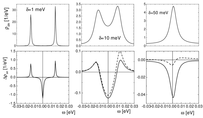
FIG. 6.: Impurity spectral density $\rho_{d\sigma}(\omega)$ (top) and change in the surface spectral density due to addition of the impurity at the impurity site $\Delta\rho_{s\sigma}(\omega)$ (bottom) for the configuration of the mirage experiment and different values of the width of the conduction levels $\delta:$ 1 meV (left), 10 meV (middle) and 50 meV (right). The dashed line shows $\Delta\rho_{s\sigma}(\omega)$ at the empty focus. Parameters as in Fig. 4 (section 5 A).

As $\delta$ increases, the two peaks in $\rho_{d\sigma}(\omega)$ merge into one (for $\delta\sim 18$ meV) and the shape of both, the Kondo resonance and the Fano antiresonance, become similar to the results of the more conventional case, described qualitatively by the simple model of section 3. The Fano dip in $\Delta\rho_{s\sigma}(\omega)$ for $\delta=50$ meV agrees well with experiment [12]. The rather symmetrical shape is due to the fact that $V_{s}$ decreasing with energy was assumed. For constant $V_{s}$, $\Delta\rho_{s\sigma}(\omega)$ is smaller for positive $\omega$ (see full line of Fig. 16). The evolution of $\rho_{d\sigma}(\omega)$ with $\delta$, described first in Ref. [38], has been confirmed by exact diagonalization plus embedding [47], and by Wilson renormalization group calculations [44].

In Fig. 6 we also show $\Delta\rho_{s\sigma}(\omega)$ at the empty focus. The comparison with the corresponding value at the focus where the impurity is located establishes the intensity of the mirage effect. For small $\delta$ the “transmission” of the Kondo effect to the empty focus is nearly perfect, because the space dependence follows closely the density of the state 42 which has maxima at the foci (see Fig. 8). As $\delta$ increases, the intensity of the mirage decreases as a consequence of interference effects described in the next section.

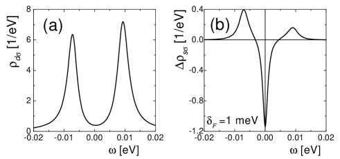
FIG. 7.: (a) Impurity spectral density and (b) $\Delta\rho_{s\sigma}(\omega)$ at the impurity site as a function of energy for $\delta_{j}=\delta_{F}(\epsilon_{j}-\epsilon_{b})/(\epsilon_{F}-\epsilon_{b})$ with $\delta_{F}=1$ meV. Other parameters are $V_{s}=0.45$ eV, $\delta_{b}=35$ meV, $E_{d}^{eff}=7$ meV, and $U=1$ eV.

The introduction of moderate hybridization of the impurity with bulk states does not affect the need to include a non vanishing $\delta$ to be able to obtain a reasonable agreement with experiment. In Fig. 7 we show again both densities for $\delta=1$ meV and parameters such that the strength of the hybridization of the impurity with bulk and surface states is approximately the same [92]. The peaks in $\rho_{d\sigma}(\omega)$ and $\rho_{s\sigma}(\omega)$ are broadened with respect to the previous case, but again the dip in $\Delta\rho_{s\sigma}(\omega)$ is not a Fano antiresonance, but correspond to minus the peak in $\rho_{s\sigma}(\omega)$ at $\epsilon_{F}$ in absence of the impurity.

VII The space dependence of $dI/dV$

While scattering theories based on a phenomenological phase shift for the scattering at the atoms of the boundary and the impurity describe quantitatively the space dependence [31, 36, 37], approaches based on wave functions of a corral (with continuous boundaries) usually bring more insight into the underlying physics [32, 33, 38]. For example the prediction of mirages out of the foci of elliptical corrals are somewhat hidden in the scattering approaches. Instead, mirages observed in a circular corral [13] were inspired by the extrema of the wave functions of the degenerate $37^{th}$ and $38^{th}$ conduction eigenstates of a hard-wall circular corral, and were calculated with our many-body approach for a circular corral with soft walls [52, 53].

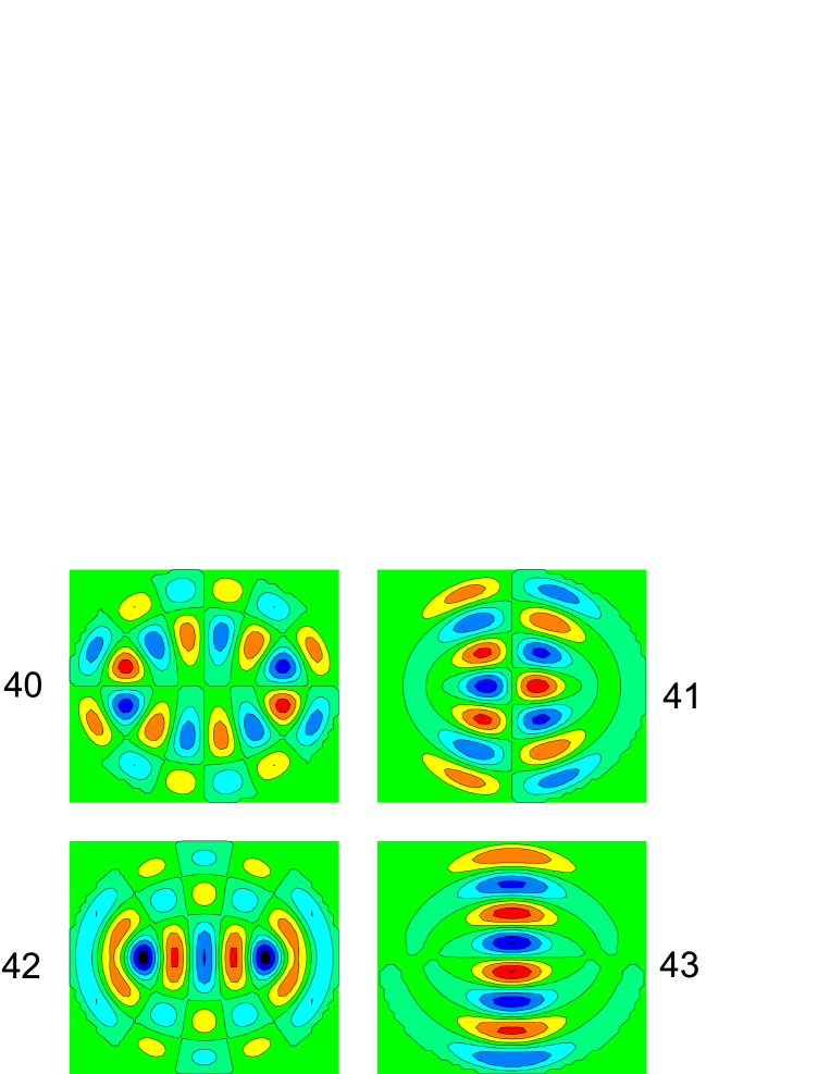
FIG. 8.: Contour plot of the wave functions of an elliptical corral with semimajor axis $a=7.13$ nm and eccentricity $e=1/2$ which lie close to the Fermi energy.

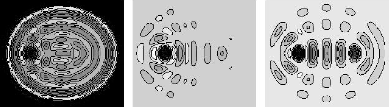
FIG. 9.: Contour plot of $dI/dV$ in the elliptical corral with $a=7.13$ nm and $e=1/2$ for $\delta=50$ meV (left), $\Delta dI/dV$ for ${\delta=50}$ meV (middle), and $\Delta dI/dV$ for $\delta=20$ meV (right). The applied voltage is 10 mV. Other parameters as in Fig. 4 (section 5 A).

Having in mind the most studied case of the mirage effect: a Co impurity placed at one focus of an elliptical corral with $e=1/2$ built on a Cu(111) surface [12], we have calculated the differential conductance $dI/dV(R_{t},R_{i},V)$ as a function of the tip position $R_{t}$, for the impurity position fixed at the left focus [$R_{i}=(-0.5a,0)$] and voltage $V=10$ mV. We used Eqs. (12), (20) and (41). We have taken $p=q=0$, since they are important only near the impurity [74]. Therefore the results depend on the impurity Green’s function $G_{d}(\omega)$ calculated as is section 4 A, and mainly on the unperturbed surface Green’s function $G_{s}^{0}(R_{1},R_{2},\omega)$. To calculate the latter we used Eq. (41) with the corral wave functions $\varphi_{j}^{c}(R)$ calculated as in Ref. [93]. The wave functions of the states which lie nearer to the Fermi energy are shown in Fig. 8. The wave functions can be classified by symmetry into the four irreducible representations of the point group $C_{2v}$, according to the parity under reflection through the major (minor) axis $\sigma_{y}$ ($\sigma_{x}$). In particular each of the shown wave functions belongs to a different representation. The state 42, which lies at the Fermi energy is even under both reflections, 40 is odd under both of them, 41 is even under $\sigma_{y}$ and odd under $\sigma_{x}$, and 43 is odd under $\sigma_{y}$ and even under $\sigma_{x}$.

The results presented in Fig. 9 were obtained for $V_{b}=0$, but quite similar results come out if $V_{s}$ is decreased by a factor $1/\sqrt{2}$ and $V_{b}$ is increased so that the contribution to the resonant level width of bulk and surface states has the same magnitude, and the width of the impurity spectral density is kept. This is not surprising since the above mentioned change of parameters practically does not affect $G_{d}(\omega)$, and then, from Eq. (20), the only change in $\Delta dI/dV(R_{t})$ for $p=q=0$ comes from a factor $V_{s}^{2}$ (see Fig. 3 of Ref. [52]). Instead, the dependence on the impurity position $R_{i}$ should be affected by the relative strength of $V_{b}$ and $V_{s}$ (see next section).

The differential conductance $dI/dV(R_{t})$ for a constant width $\delta=50$ meV of the conduction surface states is represented in Fig. 9 left. It is very similar to the observed topograph [12]. However, the latter corresponds to the total current $I$ and not to $dI/dV$. The similarity is due to the fact that $\delta$ is larger than the energy corresponding to the applied voltage $eV=10$ meV, and $dI/dV$ does not change too much in this energy scale. Comparing with Fig. 8, one sees that as a first approximation, the observed pattern can be described as a sum of the densities of the state 42 which lies at the Fermi energy $\epsilon_{F}$, and the state 43 which is $\sim eV$ above $\epsilon_{F}$. The wave function of the state 42 shows some vertical “stripes” which end in “arcs” at the extreme left and right. These essential features rotated 90 degrees describe roughly the wave function of the state 43. Therefore the structure with “arcs” at the border and “stripes” in the middle is to be expected in the sum of probability densities.

Translated into equations, this is consistent with the behavior expected from the first term of the first Eq. (20) and Eq. (41). However, this is not the whole story because the above mentioned term depends on the sum of squares of wave functions and is therefore invariant under all symmetry operations of the ellipse, while the observed topograph (and our calculated $dI/dV$) has not a defined parity under $\sigma_{x}$. The addition of the impurity breaks the symmetry under $\sigma_{x}$ and the effect of the impurity is contained completely in $\Delta G_{h}$ [see Eq. (20)]. The imaginary part of $\Delta G_{h}$ is directly proportional to $\Delta dI/dV$, which is $dI/dV$ minus the corresponding quantity for the empty corral. From Eqs. (20) and Eq. (41), it is clear that physically the effect of this subtraction is to eliminate the contribution of all states $j$ which have a negligible hybridization with the impurity $V_{s}\varphi_{j}^{c}(R_{i})$. In particular, states odd under $\sigma_{y}$ like 40 and 43 have $\varphi_{j}^{c}(R_{i})=0$ and do not participate in $\Delta dI/dV$. In practice, states like 41 which are even under $\sigma_{y}$ but have a small amplitude at the foci do not affect the result either. In Fig. 9 middle we show the “cleaned” result $\Delta dI/dV$ for the same parameters of the complete result $dI/dV$ shown at the left. Now the main features of the wave function of the state 42 can be recognized directly, particularly if the width of the conduction levels is reduced to $\delta=20$ meV (Fig. 9 right). Comparison with experiment [12] indicates that the right value of $\delta$ is in between those shown: $20$ meV $<\delta<50$ meV.

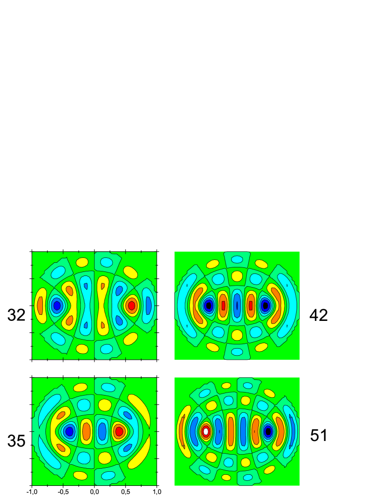
FIG. 10.: Contour plot of the wave functions of an elliptical corral with semimajor axis $a=7.13$ nm and $e=1/2$ with appreciable amplitude and the foci and close to the Fermi energy.

An analysis of the magnitude of the wave functions at the foci (which determine the hybridization strength of the impurity with the different states) shows that the space dependence of $\Delta dI/dV$ is dominated by four states. The wave functions of these states are shown in Fig. 10. While all these states are even under $\sigma_{y}$ (otherwise they would not hybridize with the impurity), only 42 is even under $\sigma_{x}$. The rest are odd under $\sigma_{x}$. This produces a negative interference between the contribution of the state 42 and the other three at the empty focus which tends to destroy the mirage effect. In simple terms, one could say that the information of the Kondo effect transmitted by the focus of the impurity by the four wave functions reaches the other focus with positive sign for the states 42 and with negative sign by the states 32, 35 and 51 so that the amplitude is reduced. Formally, this can be seen in Eqs. (20) and (41). As $\delta$ decreases, the relative contribution of the state 42 which lies at the Fermi energy increases and the size of the mirage effect also increases. This suggest to reduce $\delta$, if one can control this parameter experimentally, or to try to optimize the geometry in order to reduce the negative interference effects [38]. However, as shown in the previous section, if $\delta$ is reduced too much, the Kondo resonance and Fano antiresonance near the Fermi level are destroyed.

VIII Voltage dependence of $\Delta dI/dV$

The experimental study of the line shape of $\Delta dI/dV$ at the impurity site in different positions of one corral or in different corrals and its comparison with theory should be useful to elucidate the relative strength of the hybridization of the magnetic impurity with bulk and surface states. A greater sensitivity to geometry points towards a greater relevance of surface states. Recently, it has been argued that due to the exponential dependence of the Kondo temperature on the density of states [65], the observed line shape with approximately the same width in different situations, indicates that the hybridization with bulk states should be much more important [45]. However, the calculations of Ref. [45] are rather generic and the specific features of the corral states were not taken into account.

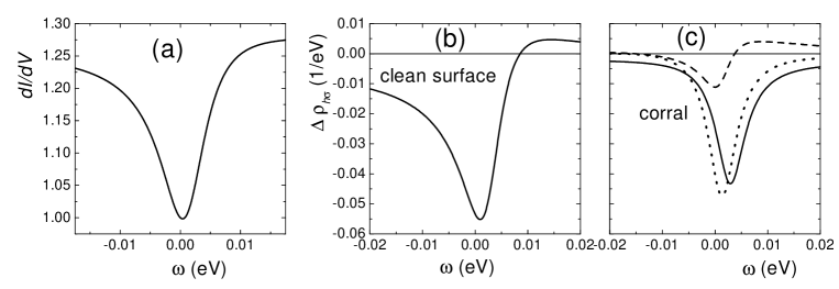
FIG. 11.: (a) Analytical function used to fit $dI/dV$ for a Co atom on a clean Cu(111) surface (Ref. 17). (b) Density of the $h_{\sigma}$ state proportional to $\Delta dI/dV$ [see Eq. (11)] for the system of (a). (c) same as (b) for a Co atom at the focus of the elliptical corral of Fig. 10, at the Co position (full line) and at the empty focus (dashed line). For comparison, the dotted line is the result for the clean surface with $q=0$. Parameters are $V_{s}=0.64$ eV, $\delta=40$ meV, $U=1$ eV and $q=0.03$.

For the case of the Cu(111) surface, to the best of our knowledge the dependence of $\Delta dI/dV$ on bias voltage has been reported only in two cases: the clean surface [12, 17] (see Fig. 4) and the elliptical corral described in the previous section, with a Co atom at one of the foci [12]. In the latter case the line shape is more symmetric, but the width is approximately the same in both cases. Both line shapes can be qualitatively described including only hybridization with surface states. In Fig. 11 we show our results obtained within perturbation theory, using Eqs. (20), with $p=0$, and $q=0.03$, to control the asymmetry of the line. Since we used here constant $V_{s}$ and surface density of states $\rho_{s}$ (as in section 3), and the nearly symmetric case $E_{d}+U/2\sim\epsilon_{F}$, the line shape for the clean surface is symmetric for $q=0$ (dotted line in Fig. 11 (c)), and a value of $q>0$ reproduces the observed asymmetry (Fig. 11 (a)). Instead, a constant $V_{s}$ in the corral case leads to an asymmetry opposite to that observed for the clean surface (like the full line of Fig. 16), while the line shape observed in the corral is symmetric. Then, in this case the effect of $q>0$ is to correct the asymmetry. It is encouraging that the same set of reasonable parameters can explain qualitatively both line shapes. The experimental $\Delta dI/dV$ has kinks around $\pm 0.01$ V which are probably due to peculiarities of the non-interacting band structure and are out of the scope of our theory [12, 17]. As shown at the bottom of Fig. 6, the width of $\Delta dI/dV$ has some variation with the width of the conduction states $\delta$. Here we have chosen $\delta=40$ meV, which as discussed in the previous section, leads to a space dependence of $dI/dV$ in agreement with experiment.

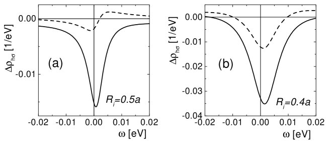
FIG. 12.: $\Delta\rho_{h\sigma}(\omega)\sim\Delta dI/dV(\omega/e)$ [see Eq. (11)] for an ellipse with $a=6.46$ nm and $e=1/2$, and two impurity positions: (a) $R_{i}$ at one focus, (b) $R_{i}=(\pm 0.4a,0)$. Full (dashed) line corresponds to the tip at $R_{i}$ ($-R_{i}$). Parameters are $\delta_{j}=\delta_{F}(\epsilon_{j}-\epsilon_{b})/(\epsilon_{F}-\epsilon_{b})$ with $\delta_{F}=40$ meV, $V_{s}=0.48$ eV, $\delta_{b}=32$ meV, $E_{d}^{eff}=7$ meV, $U=1$ eV, $p=0$ and $q=0.02$.

The rather similar line widths in the above mentioned cases seems accidental and other situations are more suitable to analyze the relative role of surface and bulk states in the formation of the Kondo resonance. In Fig. 12 we show the line shape expected in a smaller elliptical corral, with semimajor axis reduced to $a=6.46$ nm keeping the same eccentricity $e=1/2$, so that the state 35 (see Fig. 10) falls at the Fermi energy. This state has extrema at positions $R_{e}=(\pm 0.4a,0)$, and the average separation of the levels is larger than in the previous case. The surface spectral density near the Fermi level is larger at $R_{e}$ than at the foci $(\pm 0.5a,0)$. Even including the same hybridization strength of the impurity with surface and bulk states, the depth and width of $\Delta dI/dV$ is substantially larger if the impurity is placed at $R_{e}$ rather than at the foci. Note also that the intensity with the tip at the opposite point $R_{t}=-R_{i}$ is considerable larger in this case. This is due to the fact that the negative interference between states 42 and 35 explained in the previous case is substantially reduced. A stronger mirage in this geometry has been predicted before [38].

In the rest of this section, we show results for the line shape for the tip placed on the impurity and several positions of the impurity inside a circular corral of radius $r_{0}=6.35$ nm, in such a way that the degenerate states 37 and 38 lie at the Fermi level. Experiments in this corral have been done to illustrate the simultaneous presence of two mirages [13]. We use the SBMFA, because it gives the correct exponential dependence of $T_{K}$ with the coupling constant [65]. We also use the exact Eqs. (37) to (40) for the surface Green’s function instead of the approximate one Eq. (41). The SBMFA is described in section 5 B and the parameters are those taken there to fit the line shape for the clean surface.

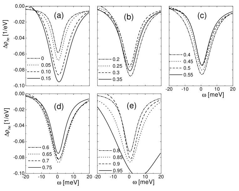
FIG. 13.: $\Delta\rho_{h\sigma}(\omega)\sim\Delta dI/dV(\omega/e)$ within SBMFA for a circular corral of radius $r_{0}=6.35$ nm at the impurity position ($R_{t}=R_{i}$), for $\delta_{F}=40$ meV, $\delta_{b}=\delta_{s}$ and different values of $|R_{i}|/r_{0}$ indicated inside each figure. Other parameters as in Fig. 4 (section 5 B).

In absence of the impurity, the density of surface conduction electrons at the Fermi energy has a pronounced relative maximum near $r=|R_{i}|=0.15r_{0}$ [52]. As shown in Fig. 13 (a), the depth and width of $\Delta dI/dV$ varies considerably as the impurity and STM tip are moved together from the center of the corral to this maximum. At the center, only the corral surface states with angular momentum projection $m=0$ can hybridize with the impurity. Since the corresponding resonances are far from the Fermi level (see Fig. 14), the Fano antiresonance for $r=0$ is more than 80% due to bulk states. In fact, doing the same calculation with $p=0$ (assuming no hopping between tip and bulk states, see Eqs. (8) and (20)), $|\Delta\rho_{h\sigma}|<0.01/$eV. Therefore for $r=0$ the bulk states play a major role not only in the formation of the Kondo state but also in the variation of the STM current $\Delta dI/dV$ which is mainly due to the current between tip and bulk states. At remote positions this Fano antiresonance of bulk states will not be observed [74]. In general, the contribution to the dip in $\Delta dI/dV$ due to bulk states (and interference with surface states), captured at the impurity by the hybridization of tip and bulk states, will be absent at a mirage point and is a natural limitation of the intensity at the mirage point (see next section). For $r/r_{0}=0.15$, the intensity of $\Delta dI/dV$ decreases to $\sim$ 40% if the tip-bulk hopping is disconnected.

Compared with the rapid variation for $r/r_{0}<0.2$, the width and magnitude of $\Delta dI/dV$ oscillates weakly with position for $0.2<$ $r/r_{0}<0.9$, with larger intensity and width for $r/r_{0}=0.4$, 0.65, and 0.85 (see Fig. 13). However, there is a dramatic increase for $r/r_{0}>0.9$, with a maximum near 0.96, as shown in Fig. 13 (e). Although unfortunately at this short distances from the boundary our theory ceases to be reliable (because of our simple assumption of a continuous boundary potential), it is instructive to relate this result with the variation of the density of surface states $\rho_{s\sigma}^{0}(r,\omega)$ at the Fermi energy $\epsilon_{F}=0$ with position. As shown in Fig. 14, there is a moderate increase in $\rho_{s\sigma}^{0}(r,\omega)$ near $\omega=0$ as $r/r_{0}$ increases from 0.15 to 0.95. This is mainly due to the contribution of resonances with high angular momentum projection which render $\rho_{s\sigma}^{0}$ rather flat in energy. Instead, for $r/r_{0}=0$, the resonances with $m=0$ are selected and they lead to the displayed oscillatory behavior.

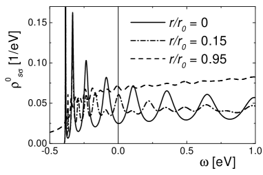
FIG. 14.: Density of unperturbed surface states $\rho_{s\sigma}^{0}(r,\omega)=-\lambda^{2}{\rm Im}[G_{s}^{0}(r,\theta,r,\theta,\omega)/\pi]$ [see Eqs. (37) to (40)] as a function of energy $\omega$ for different values of $r/r_{0}$.

The parameters of Fig. 13 correspond to an equal participation of bulk and surface states in the resonant level $\delta_{b}=\delta_{s}$. Considering the case $\delta_{b}=3\delta_{s}$, as expected, the variation of the width of the resonance with the position of the impurity is less pronounced, but otherwise the same qualitative features as before are obtained. Except for the peculiar behavior near the boundary of the corral, the greater sensitivity to the position is for $0<$ $r/r_{0}<0.15$ as before. Comparison between both cases is presented in Fig. 15. In Fig. 15 (a) and (b) we have used an intensity of the boundary potential $V_{\text{conf}}=7$, which leads to a broadening $\delta_{F}=40$ meV of the surface conduction states at the Fermi level (see section 6 A). This value leads to a space dependence in agreement with experiment (see section 7). In Fig. 15 (c) we show how the space variation is affected if the confining potential is increased to $V_{\text{conf}}=15$, leading to $\delta_{F}=20$ meV. The oscillations in the surface density of states and therefore the variation of the width of the resonance with position becomes much more pronounced. There is a tendency to a change in the line shape, similar to that of Fig. 6 for $\delta_{F}=10$ meV, which can allow to identify or rule out this regime experimentally. For other positions of the impurity (not shown), the tendency is similar to that of Fig. 13, but the particular structure for $r/r_{0}=0.95$ almost disappeared.

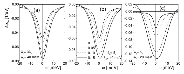
FIG. 15.: Same as Fig. 13 for (a) $\delta_{F}=40$ meV, $\delta_{b}=3\delta_{s}$, (b) $\delta_{F}=40$ meV, $\delta_{b}=\delta_{s}$ and (c) $\delta_{F}=20$ meV, $\delta_{b}=\delta_{s}$.

IX Lower bound for impurity-surface hybridization

Within our local picture for the hybridization of the impurity and tip with conduction states, a simple estimate of a lower bound for $V_{s}/V_{b}$ can be obtained from the mirage experiment in the elliptical quantum corral [12]. The ratio of the intensity of $\Delta dI/dV$ at the mirage point $I_{m}$ (for the tip position $R_{t}=-R_{i}$) to that at the impurity $I_{i}$ (for $R_{t}=R_{i}$) was reported to be $I_{m}/I_{i}\cong 1/8$. As in section 3, let us approximate $G_{b}^{0}(R_{i},R_{i},\omega)\simeq-i\pi\rho_{b}$. Also, for enough broadening of the surface conduction states $\delta\geq 40$ meV one has $G_{s}^{0}(R_{i},R_{i},\omega)\simeq-i\pi\rho_{s}$ [38]. Neglecting the tip-impurity hopping ($q=0$), using Eqs. (12) and (20) one has

$$I_{i}=-\Delta dI/dV(R_{t})\simeq C\left(\frac{V_{s}}{V_{b}}+p\frac{\rho_{b}}{\rho_{s}}\right)^{2}\rho_{d}(\omega)=C\left(\frac{V_{s}}{V_{b}}+1\right)^{2}\rho_{d}(\omega),$$ (42)

where $C=\pi V_{b}^{2}\rho_{s}^{2}$ is a constant and in the last equality we assumed that $p\rho_{b}=\rho_{s}$, so that in the absence of impurity, the tip detects bulk and surface states with the same intensity, as reported experimentally [17, 58, 59]. Now, at the mirage point one can neglect $G_{b}^{0}(R_{i},-R_{i},\omega)$ [74]. Assuming instead perfect transmission from the surface states (as if only the state 42 were relevant), one has $G_{s}^{0}(R_{i},-R_{i},\omega)=G_{s}^{0}(R_{i},R_{i},\omega)$. Since the amplitude at the mirage point is less than that for perfect transmission, one has from Eqs. (12) and (20)

$$I_{m}=-\Delta dI/dV(-R_{t})<C\left(\frac{V_{s}}{V_{b}}\right)^{2}\rho_{d}(\omega),$$ (43)

and then, from Eqs. (42) and (43)

$$\frac{V_{s}}{V_{b}}>\sqrt{\frac{I_{m}}{I_{i}}}\left(1+\frac{V_{s}}{V_{b}}\right)>\sqrt{\frac{I_{m}}{I_{i}}}+\frac{I_{m}}{I_{i}}\text{.}$$ (44)

Solving a quadratic equation, a more precise bound for $I_{m}/I_{i}=1/8$ gives $V_{s}/V_{b}>0.547$. Using $\rho_{b}\simeq 3\rho_{s}$, this implies $\delta_{s}>\delta_{b}/10$, with $\delta_{c}=\pi\rho_{c}V_{c}^{2}$. A smaller tip-bulk hopping $p$ leads to a larger lower bound for $\delta_{s}$.

X Interaction between Kondo impurities in a quantum corral

Experiments with two impurities inside an elliptical quantum corral have been done [13], but the results were not published yet. These experiments should be particularly useful as a test of the relative strength of the hybridization of the impurity with bulk and surface states, since one expects that at distances larger than $\sim$0.5 nm, the interaction between two Kondo impurities is dominated by surface states. In this section we extend previous calculations of the line shape of $\Delta dI/dV$ when there is one impurity at each focus of an elliptical corral, using the technique of exact diagonalization plus embedding, described in section 5 C [47]. Other calculations of the interaction between magnetic impurities in a corral have been made by perturbation theory in the Kondo coupling [94]. However, this technique does not work in the case we are interested of antiferromagnetic Kondo coupling $J_{K}>0$ [65].

As explained in section 5 C, the Hamiltonian is written as $H=H_{0}+$ $H^{\prime}+$ $H_{r}$. In our case the Hilbert space of $H_{0}$ contains one or two impurities and the most important surface conduction states (those represented in Fig. 10) and two additional ones (24 and 62) although they do not affect the results. $H_{r}$ describes a set of independent non-interacting bulk states which hybridize independently with the impurities and the surface conduction states. $H_{0}$ has a similar form to Eq. (2) but only contains hard-wall surface conduction states and can contain more than one impurity:

$$H_{0}=\sum_{j\sigma}\epsilon_{j}s_{j\sigma}^{\dagger}s_{j\sigma}+E_{d}\sum_{i\sigma}d_{i\sigma}^{\dagger}d_{i\sigma}+U\sum_{i}d_{i\uparrow}^{\dagger}d_{i\uparrow}d_{i\downarrow}^{\dagger}d_{i\downarrow}+\sum_{ij\sigma}\lambda V_{s}[\varphi_{j}(R_{i})d_{i\sigma}^{\dagger}s_{j\sigma}+\text{H.c.}],$$ (45)

while the effect of bulk states and the broadening of the surface states (necessary to obtain a qualitatively reasonable line shape as shown in section 6) is contained in $H^{\prime}$ which reads

$$H^{\prime}\cong t\sum_{j\sigma}(s_{j\sigma}^{\dagger}b_{j\sigma}+\text{H.c.})+V_{b}\sum_{i\sigma}(d_{i\sigma}^{\dagger}b_{i\sigma}+\text{H.c.}).$$ (46)

For the bulk states $b_{l\sigma}$ we take a constant unperturbed density of $\rho_{b}=0.05$ states/eV per spin (of the order of the density of bulk $s$ and $p$ states at $\epsilon_{F}$.[90]), but a change in $\rho_{b}$ can be absorbed in a change in $t$ and $V_{b}$. The value of $t$ controls the width of the conduction states and therefore, the intensity at the mirage point, as explained in sections 6 and 7.

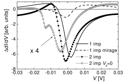
FIG. 16.: $\Delta dI/dV$ as a function of applied voltage calculated with the EDE for an elliptical corral with one or two impurities at the foci. Full line: one impurity and tip on it. Dashed line: one impurity and tip at the other foci. Solid squares: two impurities and tip on one of them. Open circles: same as before with $V_{s}$ increased by a factor $\sqrt{2}$ and $V_{b}=0$. Unless otherwise indicated parameters are $E_{d}=-0.8$ eV, $U=3$ eV (from Ref. 67), $V_{s}=1.12/\sqrt{2}$ eV, $V_{b}=1.2$ eV, $p=q=0$.

In Fig. 16, we represent the change in differential conductance for $p=q=0$ for the case in which there is one impurity at each focus, comparing two situations. In the first one $V_{b}=0$ and $V_{s}=1.12$ eV is taken to reproduce approximately the experimental width. In the second one $V_{s}$ is reduced by a factor $1/\sqrt{2}$ and $V_{b}$ increased to 1.2 eV in order that the same width and practically the same line shape is obtained. In the former case, the effect of the interaction between impurities is stronger and the line is wider and with some structure due to a partial splitting of the Kondo resonance. In the second case, the result is very similar to the sum of the spectra at both foci when only one impurity is present. This is the result expected for weak interactions.

XI Summary and discussion

Using a simple impurity Anderson model in which the particular structure of the surface states inside a corral is taken into account appropriately, the basic physics of the mirage experiments in quantum corrals [12, 13] can be understood. The resulting space and voltage dependence of the differential conductance $dI/dV$ is in good agreement with experiment. The voltage dependence of $dI/dV$ observed for one Co atom on a clean Cu(111) surface and for a Co atom at the focus of an elliptical corral built on that surface can both be explained with the same set of parameters (see Fig. 11).

While the space dependence of $dI/dV$ is mainly determined by non-interacting conduction electron Green’s functions, the calculation of the dependence of $dI/dV$ on bias voltage is a non trivial many-body problem in which the particular structure of the conduction electrons for surface states introduces additional complications. Single-particle scattering theories were successful in explaining the space dependence of $dI/dV$ [31, 36, 37], but the voltage dependence is actually used to adjust a phenomenological energy dependent phase shift. Therefore the differences in the line shape as a function of the applied voltage in different structures (like the above mentioned between an impurity on a clean surface or inside the corral) cannot by accounted for. In contrast, the many-body treatment is very difficult to implement for open structures, while one-body scattering theory assuming simple interactions, allows not only to calculate but also to optimize open structure to obtain multiple mirages or other desired effects [95]. On the other hand, our approach leads to very good agreement with the space dependence of $dI/dV$ (see Fig. 9) except perhaps for the finest details which we did not attempt to fit. In addition, it allows to understand the basic observed features, including the mirage effects and its intensity, in terms of the interference of wave functions in the corral (see section 7).

Experiments in which the change in differential conductance after addition of one impurity in a quantum corral $\Delta dI/dV$ is measured should be able to discern the relative importance of surface and bulk states in the formation of the Kondo singlet. Measurements in circular corrals, easier to handle theoretically, would be useful. In section 8 we presented some results for this case. In addition, the change of $\Delta dI/dV$ when more than one impurity is present in the corral is very sensitive to the surface-impurity hybridization. The observation of a quantum mirage establishes a lower bound for this hybridization which we have estimated.

The calculations presented here are for $T=0$. Within perturbation theory, the results can be extended easily to $T\neq 0$. Some results were presented in Ref. [52]. Important changes occur in the scale of the Kondo temperature, but the behavior is similar to that already known for the simple case explained in section 3.

An improvement of the many-body theory requires a better knowledge of the hybridization of the impurity with surface and bulk states and their wave vector dependence (which we have neglected). The wave vector dependence is expected from a jellium model [55]. In particular for the states near the Fermi energy $\epsilon_{F}$ and wave functions decaying as $\exp(-\kappa z)$ out of the surface, one expects $k_{||}^{2}-$ $\kappa^{2}$ constant and therefore a smaller wave vector parallel to the surface $k_{||}$ implies a weaker decay rate $\kappa$ in the perpendicular $z$ direction, and therefore a larger hybridization with impurity and tip. For surface states near $\epsilon_{F}$, $k_{||}$ is small and one would expect a weaker decay for surface than bulk states. This suggests a stronger relative hybridization of bulk states with the impurity in comparison with the tip, because the former is closer to the surface. This would be consistent with the fact that the hybridization of the tip with surface and bulk states is of the same order [17, 58, 59], and the proposal that bulk states dominate the hybridization with the impurity [17, 18, 45, 54]. However, more detailed calculations of the matrix elements found oscillations of the matrix elements with $z$, and a stronger relevance of surface states in the formation of the Kondo state [56] and in the distance dependence of the observed $dI/dV$ for magnetic impurities on clean (111) surfaces [56, 57].

We have shown that the width of the surface conduction electrons $\delta$ plays a crucial role in the many-body theory (see section 6). We have calculated this width for a circular confinement potential and found that it increases linearly with energy [52]. However, we assumed that for a clean surface the surface states are well defined for all wave vectors and this is not the case for energies above the Fermi energy [30]. Since localization involves a participation of all wave vectors, there is a contribution to the width brought by the states of larger wave vector which we have neglected. However, since most of the physics depends on the value of $\delta$ at the Fermi energy and we took it as a parameter, our conclusions are not affected.

Correlation functions of impurities inside a quantum corral have been studied previously [47, 48, 52, 94, 95]. For perfect confinement a strong enhancement should occur. However, for realistic broadening of the surface conduction states, and distances of the order of several nm involved in the mirage experiments, we expect that the single ion physics dominate the RKKY interactions, and no significant magnetic correlations are present [52].

REFERENCES

- [1] D. Goldhaber-Gordon, H. Shtrikman, D. Mahalu, D. Abusch-Magder, U. Meirav, and M. A. Kastner, Nature 391, 156 (1998).
- [2] S. M. Cronenwet, T. H. Oosterkamp, and L. P. Kouwenhoven, Science 281, 540 (1998).
- [3] D. Goldhaber-Gordon, J. Göres, M. A. Kastner, H. Shtrikman, D. Mahalu, and U. Meirav, Phys. Rev. Lett. 81, 5225 (1998).
- [4] W.G. van der Wiel, S. de Franceschi, T. Fujisawa, J.M. Elzerman, S. Tarucha, and L.P. Kowenhoven, Science 289, 2105 (2000).
- [5] P.W. Anderson, Phys. Rev. 124, 41 (1961).
- [6] A. C. Hewson, in The Kondo Problem to Heavy Fermions (Cambridge, University Press, 1993).
- [7] W. Izumida, O. Sakai, and S. Suzuki, J. Phys. Soc. Jpn. 70, 1045 (2001).
- [8] T.A. Costi, Phys. Rev. B 64, 241310(R) (2001).
- [9] V. Fano, Phys. Rev. 124, 1866 (1961).
- [10] J. Li, W.-D. Schneider, R. Berndt, and B. Delley, Phys. Rev. Lett. 80, 2893 (1998).
- [11] V. Madhavan, W. Chen, T. Jamneala, M.F. Crommie, and N.S. Wingreen, Science 280, 567 (1998).
- [12] H.C. Manoharan, C.P. Lutz, and D.M. Eigler, Nature (London) 403, 512 (2000).
- [13] H.C. Manoharan, PASI Conference, Physics and Technology at the Nanometer Scale (Costa Rica, June 24 - July 3, 2001).
- [14] T. Jamneala, V. Madhavan, W. Chen, and M.F. Crommie, Phys. Rev. B 61, 9990 (2000).
- [15] V. Madhavan, W. Chen, T. Jamneala, M.F. Crommie, and N.S. Wingreen, Phys. Rev. B 64, 165412 (2001).
- [16] K. Nagaoka, T. Jamneala, M. Grobis, and M.F. Crommie, Phys. Rev. Lett. 88, 077205 (2002).
- [17] N. Knorr, M. A. Schneider, L. Diekhöner, P. Wahl, and K. Kern, Phys. Rev. Lett. 88, 096804 (2002).
- [18] M.A. Schneider, L. Vitali, N. Knorr, and K. Kern, Phys. Rev. B 65, 121406 (2003).
- [19] P. Wahl, L. Diekhöner, M. A. Schneider, L. Vitali, G. Wittich, and K. Kern, Phys. Rev. Lett. 93, 176603 (2004).
- [20] B. R. Bulka and P. Stefanski, Phys. Rev. Lett. 86, 5128 (2001).
- [21] K. Kang, S. Y. Cho, J. J. Kim, and S. C. Shin, Phys. Rev. B 63, 113304 (2001).
- [22] M. E. Torio, K. Hallberg, A. H. Ceccatto, and C. R. Proetto, Phys. Rev. B 65, 085302 (2002).
- [23] A.A. Aligia and C.R. Proetto, Phys. Rev. B 65, 165305 (2002).
- [24] M. E. Torio, K. Hallberg, S. Flach, A.E. Miroshnichenko, and M. Titov, Eur. Phys. J. B 37, 399 (2004).
- [25] A.A. Aligia and M.A. Salguero, Phys. Rev. B 70, 075307 (2004).
- [26] A. A. Aligia, K. Hallberg, B. Normand, and A. P. Kampf, Phys. Rev. Lett. 93, 076801 (2004).
- [27] D.M. Eigler and E.K. Schweizer, Nature (London) 344, 524 (1990).
- [28] M.F. Crommie, C.P. Lutz, and D.M. Eigler, Science 262, 218 (1993).
- [29] E.J. Heller, M.F. Crommie, C.P. Lutz, and D.M. Eigler, Nature (London) 369, 464 (1994).
- [30] S.L. Hulbert, P.D. Johnson, N.G. Stoffel, W.A. Royer, and N.V. Smith, Phys. Rev. B 31, 6815 (1985).
- [31] G.A. Fiete and E.J. Heller, Rev. Mod. Phys. 75, 933 (2003).
- [32] M. Weissmann and H. Bonadeo, Physica E (Amsterdam) 10, 44 (2001).
- [33] D. Porras, J. Fernández-Rossier, and C. Tejedor, Phys. Rev. B 63, 155406 (2001).
- [34] M. Schmid and A.P. Kampf, cond-mat/0308115.
- [35] D.K. Morr and N.A. Stavropoulos, Phys. Rev. B 67, 020502 (2003).
- [36] O. Agam and A. Schiller, Phys. Rev. Lett. 86, 484 (2001).
- [37] G.A. Fiete, J. S. Hersch, E. J. Heller, H.C. Manoharan, C.P. Lutz, and D.M. Eigler, Phys. Rev. Lett. 86, 2392 (2001).
- [38] A.A. Aligia, Phys. Rev. B 64, 121102(R) (2001).
- [39] A.A. Aligia, Phys. Status Solidi (b) 230, 415 (2002).
- [40] N. Andrei, K. Furuya, and J. Lowenstein, Rev. Mod. Phys. 55, 331 (1983).
- [41] A.M. Tsvelik and P.B. Wiegmann, Adv. Phys. 32, 453 (1983).
- [42] A.A. Aligia, C. A. Balseiro and C. R. Proetto, Phys. Rev. B 33, 6476 (1986).
- [43] K.G. Wilson, Rev. Mod. Phys. 47, 773 (1975).
- [44] P. Cornaglia and C.A. Balseiro, Phys. Rev. B 66, 174404 (2002).
- [45] P. Cornaglia and C.A. Balseiro, Phys. Rev. B 66, 205420 (2003).
- [46] A.K. Zhuravlev, V.Yu. Irkhin, M.I. Katsnelson, and A.I. Lichtenstein, Phys. Rev. Lett. 93, 236403 (2004).
- [47] G. Chiappe and A.A. Aligia, Phys. Rev. B 66, 075421 (2002); ibid 70, 129903(E) (2004).
- [48] K. Hallberg, A.A. Correa, and C.A. Balseiro, Phys. Rev. Lett. 88, 066802 (2002).
- [49] W.B. Thimm, J. Kroha, and J. von Delft, Phys. Rev. Lett. 82, 2143 (1999).
- [50] The description of the Green’s function of the surface conduction eigenstates as a sum of resonances can be demonstrated under quite general assumptions [51] and has been worked out in detail for the circular corral [52, 53].
- [51] G. García Calderón, Nucl. Phys. A 261, 130 (1976).
- [52] A. Lobos and A.A. Aligia, Phys. Rev. B 68, 035411 (2003).
- [53] A. Lobos and A.A. Aligia, in Concepts in Electron Correlation, A.C. Hewson and V. Zlatić (eds.) (Kluver Academic Publishers, Netherlands, 2003), p. 229-237.
- [54] M. A. Barral, A. M. Llois, and A. A. Aligia, Phys. Rev. B 70, 035416 (2004).
- [55] M. Plihal and J.W. Gadzuk, Phys. Rev. B 63, 085404 (2001).
- [56] C.-Y. Lin, A.H. Castro Neto and B.A. Jones, Phys. Rev. B 71, 035417 (2005).
- [57] J. Merino and O. Gunnarson, Phys. Rev. Lett. 93, 156601 (2004).
- [58] L. Bürgui, O. Jeandupeux, A. Hirstein, H. Brune, and K. Kern, Phys. Rev. Lett. 81, 5370 (1998).
- [59] O. Jeandupeux, L. Bürgui, A. Hirstein, H. Brune, and K. Kern, Phys. Rev. B 59, 15926 (1999).
- [60] K. Yosida and K. Yamada, Prog. Theor. Phys. Suppl. 46, 244 (1970); Prog. Theor. Phys. 53, 1286 (1975); K. Yamada, ibid 53, 970 (1975).
- [61] B. Horvatić, D. Šokčević, and V. Zlatić, Phys. Rev. B 36, 675 (1987).
- [62] V. Ferrari, G. Chiappe, E.V Anda and M. Davidovich, Phys. Rev. Lett. 82, 5088 (1999)
- [63] C.A. Büsser, E. V. Anda, M. Davidovich and G. Chiappe, Phys. Rev. B 62, 9907 (2000).
- [64] G. Chiappe and J.A. Verges, J. Phys. Condens. Matter 15, 8805 (2003).
- [65] In the ordinary Anderson model, for small enough hybridization one has , where , is the density of states per spin at the Fermi level, and is the Kondo coupling [40, 41, 42].
- [66] P. Coleman, Phys. Rev. B 29, 3035 (1984).
- [67] O.Újsághy, J. Kroha, L. Szunyogh, and A. Zawadowski, Phys. Rev. Lett. 85, 2557 (2000).
- [68] J. Merino and O. Gunnarson, Phys. Rev. B 69, 115404 (2004).
- [69] T.A. Costi, A.C. Hewson, and V. Zlatić, J. Phys. Condens. Matter 6, 2519 (1994).
- [70] A. Levy-Yeyati, A. Martín-Rodero, and F. Flores, Phys. Rev. Lett. 71, 2991 (1993); references therein.
- [71] A. Schiller and S. Hershfield, Phys. Rev. B 61, 9036 (2000).
- [72] G.D. Mahan, Many Particle Physics (Plenum, New York, 1981).
- [73] J. Wagner, W. Hanke, and D.J. Scalapino, Phys. Rev. B 43, 10517 (1991).
- [74] The bulk Green’s function contributes a uniform background to [Eq. (12)] through the second term of the first Eq. (20). In addition, it has a contribution to through the second Eq. (20) which is important only when tip and impurity are close to each other because at distances larger than a few nm [55, 57].
- [75] E.S. Sorensen and I. Affleck, Phys. Rev. B 53, 9153 (1996).
- [76] V. Barzykin and I. Affleck, Phys. Rev. B 57, 432 (1998).
- [77] P. Coleman, cond-mat/0206003
- [78] I. Affleck and P. Simon, Phys. Rev. Lett. 86, 2854 (2001).
- [79] A.A. Aligia, Phys. Rev. B 66, 165303 (2002).
- [80] Y. Shimada, H. Kasai, H. Nakanishi, W.A. Dino, A. Okiji. and Y. Hasegawa, J. Appl. Phys. 94, 334 (2003).
- [81] H. Kajueter and G. Kotliar, Phys. Rev. Lett. 77, 131 (1996).
- [82] R. N. Silver, J. E. Gubernatis, D. S. Sivia, and M. Jarrell, Phys. Rev. Lett. 65, 496 (1990).
- [83] M. Weissmann and A.M. Llois, Phys. Rev. B 63, 113402 (2001).
- [84] The decrease (increase) in for fixed leads to a smaller (larger) and to keep the experimentally observed width of the Fano antiresonance, but has no other important consequences.
- [85] D. C. Langreth, Phys. Rev. 150, 516 (1966).
- [86] D.M. Newns and N. Read, Adv. Phys. 36, 799 (1987).
- [87] H. Hellmann, in Einführung in die Quantumchemie (Deuticke, Leipzig, 1937), p. 285; R. P. Feynman, Phys. Rev. 56, 340 (1939).
- [88] D.N. Zubarev, Sov. Phys. Usp. 3, 329 (1960) [Usp. Fiz. Nauk. 71, 71 (1960].
- [89] V.L. Moruzzi, J.F. Janak, and A.R. Williams, Calculated electronic properties of metals (Pergamon Press, New York, 1978).
- [90] A. Euceda, D.M. Bylander, and L. Kleinman, Phys. Rev. B 28, 528 (1983).
- [91] If the Fermi level falls between two energies of the conduction states, a peak is present at for , but in any case, the structure of does not show the features that correspond to the continuous conduction density of states [49].
- [92] The parameters were modified so that the contribution of and to the width of the Fano antiresonance for meV is the same.
- [93] K. Nakamura and H. Thomas, Phys. Rev. Lett. 61, 247 (1988).
- [94] A. Correa, K. Hallberg, and C.A. Balseiro, Europhys. Lett. 58, 899 (2002).
- [95] A.A. Correa, F.A. Reboredo, and C.A. Balseiro, Phys. Rev. B 71, 035418 (2005).