Hierarchical Characterization of Complex Networks

Abstract

While the majority of approaches to the characterization of complex networks has relied on measurements considering only the immediate neighborhood of each network node, valuable information about the network topological properties can be obtained by considering further neighborhoods. The current work discusses on how the concepts of hierarchical node degree and hierarchical clustering coefficient (introduced in cond-mat/0408076), complemented by new hierarchical measurements, can be used in order to obtain a powerful set of topological features of complex networks. The interpretation of such measurements is discussed, including an analytical study of the hierarchical node degree for random networks, and the potential of the suggested measurements for the characterization of complex networks is illustrated with respect to simulations of random, scale-free and regular network models as well as real data (airports, proteins and word associations). The enhanced characterization of the connectivity provided by the set of hierarchical measurements also allows the use of agglomerative clustering methods in order to obtain taxonomies of relationships between nodes in a network, a possibility which is also illustrated in the current article.

1 Introduction

Graph theory and statistical mechanics are well-established areas in mathematics and physics, respectively. Since its beginnings in the XVIII century, with the solution of the bridges problem by L. Euler, graph theory has progressed all the way to the forefront of theoretical and applied investigations in mathematics and computer science. Much of the importance of this broad area stems from the generality of graphs as representational models. As a matter of fact, most discrete structures including matrices, trees, queues, among many others, are but particular cases of graphs. The potential of graphs is further extended by models where features are assigned to nodes, different types of nodes and/or edges are allowed to co-exist, synchronization schemes are incorporated, and so on (see, for instance, [1]). At the same time, statistical mechanics, also drawing on a rich past of accomplishments, provides concepts and tools for bridging the gap between dynamics in the micro and macro realms. Of particular interest have been the investigations on phase transitions and complex systems, which represent a major area of development today.

While graph theory provides effective means for characterizing, modeling and simulating the structure of natural phenomena, statistical mechanics contains the methods for analyzing the dynamics of natural phenomena along several scales. The novel area of complex networks [2, 1] can be understood as a fortunate intersection between those two major areas, therefore allowing a natural and powerful means for integrating structure and dynamics. With origins extending back to the pioneering developments of Flory [3], Rapoport [4] and Erdös and Rényi [5], the area of complex networks was boosted more recently by the advances by Watts and Strogatz [6, 7] and Barabási and collaborators [8].

Complex network investigations frequently involve the measurement of topological features of the analyzed structures, such as the node degree (namely the number of edges attached to a node) and the clustering coefficient (quantifying the connectivity among the immediate neighbors of a node). Although degenerated, in the sense that they do not allow a one-to-one identification of the possible network architectures, such a pair of measurements does provide a rich characterization of the connectivity of the networks. As a matter of fact, particularly interesting network models, such as the small-world [1, 2, 7, 6] and scale-free (Barabási-Albert) [2, 1, 8], are characterized in terms of specific types of node degree distributions (logarithmic and power-law, respectively).

Although such distributions emphasize important properties of the analyzed networks, further valuable topological information can be gathered not only by considering the clustering coefficient, but also by analyzing such features along the hierarchical levels of the networks [9, 10]. While some attention has been focused on the relevant issue of hierarchy in complex networks (e.g. [11, 12, 13, 17, 18, 19, 20, 21, 22, 23, 24, 28, 26, 27]), and hierarchical extensions of the node degree and clustering coefficient were only more recently formalized in [9, 10] by using concepts derived from mathematical morphology [25, 29, 30] including dilations and distance transforms in graphs. Despite their recent introduction, such concepts have already yielded valuable results when applied to essentiality of protein-protein interaction networks [37], bone structure characterization [38], and community finding [32, 33].

The purpose of the current article is to review and further extend the concepts of hierarchical measurements, which is done by the consideration of the concepts of radial reference system and hierarchical common degree, as well as the introduction of the measurements of hierchical edge degree, inter-ring degree, intra-ring degree, convergence ratio, and emphedge clustering coefficient. The extensions of these measurement (excluding the clustering coefficient) to weighted and directed networks are also described in this work. We start by presenting the basic concepts and discussing hierarchies in complex networks in terms of virtual nodes and proceed by describing, interpreting and discussing the hierarchical measurements. An analytical characterization of the general shape of the hierarchical node degree in random networks is also presented, and the potential of the reported concepts and methods is illustrated with respect to the characterization of simulated random, scale-free and regular network models. Such a potential is further illustrated with respect to real networks, including word associations, airports, and protein-protein interactions. Because the hierarchical measurements provide a rich characterization of the connectivity around each network node, it becomes possible to use clustering methods [15, 14] in order to organize the nodes in a network into a taxonomical scheme reflecting the similarities between their connectivity. This possibility is also illustrated in the present article.

2 Notation and Basic Concepts

Let the graph or network $\Gamma$ of interest contain $N$ nodes and $e$ edges, and the connections between any two nodes $i$ and $j$ be represented as $(i,j)$. Although non-oriented graphs are assumed henceforth, all reported concepts and methods can be immediately extended to digraphs and weighted networks. We henceforth assume the complete absence of loops (i.e. self-connections). A non-oriented graph can be completely specified in terms of its adjacency matrix $K$, with each connection $(i,j)$ implying $K(i,j)=K(j,i)=1$. The absence of a connection between nodes $i$ and $j$ is represented as $K(i,j)=K(j,i)=0$. Now, the node degree $k(i)$ of a node $i$ of $\Gamma$ can be defined as

$$k(i)=\sum_{j=1}^{N}K(i,j)=\sum_{j=1}^{N}K(j,i).$$ (1)

Observe that the degree of node $i$ corresponds to the number of edges attached to that node, representing a direct measurement of the connectivity of that specific node. Indeed the overall connectivity of a specific network can be quantified in terms of its average node degree $\left<k\right>$. While a random network is characterized by a typical average node degree with relatively low standard deviation, a scale-free model will present a power-law log-log distribution of node degrees, favoring the existence of hubs (i.e. nodes with high node degree).

The clustering coefficient of a network node $i$ can be defined as quantifying the connectivity among the immediate neighbors of $i$, which are henceforth represented by the set $R_{1}(i)$. More specifically, in case that node has $n_{1}(i)$ immediate neighbors (i.e., the cardinality of $R(i)$), implying a maximum number $e_{T}(i)=n_{1}(n_{1}-1)/2$ of connections between such nodes, and $e(i)$ connections are observed among such neighbors, the clustering coefficient of $i$ can be calculated as

$$cc(i)=\frac{e(i)}{e_{T}(i)}=2\frac{e(i)}{n_{1}(i)(n_{1}(i)-1)}.$$ (2)

Observe that $0\leq cc(i)\leq 1$, with the minimum and maximum values being achieved for complete absence of connections (for $cc(i)=0$) and complete connectivity among the neighbors of $i$ (for $cc(i)=1$).

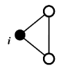
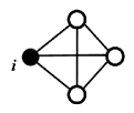
Figure 1: Three situations yielding the same clustering coefficient (equal to 1) for the reference node $i$. 

Although the clustering coefficient provides a powerful indication about the connectivity among the neighbors of the reference node, several different situations (see Figure 1) may yield the same clustering coefficient value (1 for these examples), which is a consequence of the fact that this measurement is relative to the total number of connections among the elements of $S(i)$. Such situations can be distinguished by considering the respective value of $n_{1}(i)$.

3 Virtual Edges and Hierarchies

Consider the situation depicted in Figure 2, where a reference node $i=1$ is connected to several other network nodes. The set of immediate neighbors of $i$, hence $R_{1}(i)$, is identified by the innermost ellipsis. Observe that although no connection is observed between nodes $i$ and $j$, information from the former node can propagate to the latter through the relay node $r$, which is indicated by the virtual edge [9] shown as a dashed line.

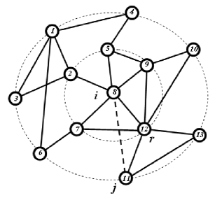
Figure 2: A small network and a reference node $i$. The virtual edge between nodes $i$ and $j$, one of the many of such a kind in this network, is represented by the dashed line. 

In the case of weighted networks, the virtual edges may take into account the cumulative effect of the respective weights. For instance, in case we had in Figure 3 $W(i,r)=3$ and $W(r,j)=4$, the weight of the virtual edge extending from $i$ to $j$ would be $W(i,j)=(3)(4)=12$.

The concept of virtual edge can be immediately extended by considering further distances $d$ from the reference node. Such an extension can be naturally defined in terms of the weight matrix $W$ representing the complex network of interest (observe that $W=K$ for weightless networks). Let $\vec{v}(i)$ be a column vector with $N$ elements equal to zero, except that at the $i-th$ position (recall that $i$ is the label of the reference node), which is assigned unit value. Let the vector $\vec{v}_{1}(i)$ be defined as

$$\vec{v}_{1}(i)=W\vec{v}(i),$$ (3)

and let the generalized Kronecker delta $\vec{a}=\delta(\vec{b})$ be the operator acting on a vector $\vec{a}$ in order to produce a vector $\vec{b}$ such that each element $b(j)$ of $\vec{b}$ is one if and only $a(j)$ is different from zero, and zero otherwise. By applying such operator on $\vec{v}_{1}(i)$ we obtain

$$\vec{p}_{1}(i)=\delta(\vec{v}_{1}(i)).$$ (4)

The set of immediate neighbors of $i$, i.e. $R_{1}(i)$, can now be obtained as corresponding to the indices of the elements of $\vec{p}_{1}(i)$ which are equal to 1. For example, we have for the situation depicted in Figure 3 that $R_{1}(i=8)=\{2,5,7,9,12\}$.

The above matrix framework can be extended to any neighborhood of $i$ by introducing the vector $\vec{v}_{d}(i)$ defined as

$$\vec{v}_{d}(i)=W^{d}\vec{v}(i).$$ (5)

The weights of the virtual edges between $i$ and the remainder network nodes at distance $d$ are given by the successive entries of $\vec{v}_{d}$, i.e. $W_{d}(i,j)=v_{d}(j)$. Observe that the distance $d$ between two nodes $i$ and $j$ is henceforth understood as corresponding to the number of edges along the shortest path between those two nodes.

The set of neighbors of $i$ placed at distances varying from 0 to $d$ from the reference node $i$, henceforth represented as $B_{d}(i)$ and referred to as the ball of radius $d$ centered at $i$, can be verified to correspond to the non-zero entries in the vector $\vec{p}_{d}(i)$ defined as follows

$$\vec{p}_{d}(i)=\delta\left(\sum_{j=1}^{d}\vec{p}_{j}(i)+\vec{v}(i)\right).$$ (6)

For instance, the ball of radius 2 centered at $i=8$ in Figure 2 corresponds to the whole network in that figure. Now, the set of network nodes which are exactly at distance $d$ from the reference node $i$ can be obtained as the unit entries in the vector

$$\vec{r}_{d}(i)=\vec{p}_{d}(i)-\vec{p}_{d-1}(i).$$ (7)

The set obtained from the above vector has also been called [10] the ring of radius $d$ centered at $i$, being henceforth represented as $R_{d}(i)$. Observe that the ring of radius 2 centered at $i=8$ in Figure 2 is $R_{2}(8)=\{1,3,4,6,10,11,13\}$.

The subnetwork defined by the nodes at a specific ring $R_{d}(i)$, together with the edges between them, is henceforth represented as $\gamma_{d}(i)$. We are now ready to define the hierarchical level $d$ of a complex network as corresponding to the nodes in $\gamma_{d}(i)$ and the edges extending from such nodes and the nodes in $\gamma_{d+1}(i)$. The two hierarchical levels of nodes existing in the network shown in Figure 2 are identified by the inner and outermost ellipsis, respectively. Observe that the hierarchies $d$ provide a radial reference frame or coordinate system which can be used to partially identify nodes and edges with respect to the reference node $i$. The concept o hierarchy in a complex network is also related to the concept of roles [34] and the distance transform [29, 30] of the nodes in the original network $\Gamma$ with respect to the reference node [10].

Observe that statistics of the number of hierarchical levels $d$ while considering several nodes in a complex network provide a valuable characterization of its topology. Generally speaking, $d$ tends do increase with the density of connections up to a peak, decreasing afterwards. At the same time, as will become clear along the remainder of this article, the more connected the network is, the less hierarchical levels it tends to have. It should be also observed that algorithmic implementation of hierarchy identification, such as those reported in [9] and [10] (see also [35]), are typically more computationally efficient than the use of the matrix arithmetic presented in this Section.

4 Hierarchical Measurements

The concept of hierarchical level introduced above allows a natural and powerful extension of traditional measurements such as the node degree and clustering coefficient. This section defines such features as well as ancillary measurements which can be used in order to obtain a more complete characterization of complex networks. The considered measures can be generalized for weighted networks taking some modifications as described along the measures. When considering oriented graphs, a new network can be obtained retrieving only the In or Out connections of each node.

The hierarchical node degree of a reference node $i$ at distance $d$ is henceforth defined as corresponding to the number of edges extending between the nodes in $R_{d}(i)$ and $R_{d+1}(i)$. This measurement is henceforth represented as $k_{d}(i)$. As an example, in Figure 2 we have that $k_{0}(8)=5$ (corresponding to the traditional node degree) and $k_{1}(8)=8$. Observe that the hierarchical node degree is not averaged among the number of nodes in $R_{d}(i)$. Actually, this measurement can be understood as the traditional node degree where the reference node is understood as corresponding to the ball $B_{d}(i)$ (i.e. the nodes in this ball are merged into a subsumed node). This measure can be extended to weighted networks by taking the sum of the weight values for every connection between these nodes and the nodes of the next level.

Let the number of edges in the subnetwork $\gamma_{d}(i)$ be expressed as $e_{d}(i)$, and the number of elements of the ring $R_{d}(i)$ be represented as $n_{d}(i)$. The hierarchical clustering coefficient of node $i$ at distance $d$, hence $cc_{d}(i)$, can be obtained in terms of the immediate generalization of Equation 2

$$cc_{d}(i)=2\frac{e_{d}(i)}{n_{d}(i)(n_{d}(i)-1)}.$$ (8)

For node $i=8$ in the simple network shown in Figure 2 we have that $cc_{1}(8)=0.3$ and $cc_{2}(8)\approx 0.19$.

Other interesting hierarchical measurements which can be obtained with respect to the reference node $i$ and which can be used to diminish the degeneracy of the node degree and clustering coefficient include the following:

Convergence ratio ($C_{d}(i)$): Corresponds to the ratio between the hierarchical node degree of node $i$ at distance $d$ and the number of nodes in the ring at next level distance, i.e.

$$C_{d}(i)=\frac{k_{d}(i)}{n_{d+1}(i)}.$$ (9)

This measurement quantifies the average number of edges received by each node in the hierarchical level $d+1$. We have necessarily that $C_{0}(i)=1$ for whatever node selected as the reference $i$. In the case illustrated in Figure 2, we have $C_{0}(8)=1$ and $C_{1}(8)=8/7$, indicating a low level of edge convergence into the nodes in $R_{d}(i)$.

Intra-ring degree ($A_{d}(i)$): This measurement is obtained by taking the average among the degrees of the nodes in the subnetwork $\gamma_{d}(i)$. Observe that only those edges between the nodes in such a subnetwork are considered, therefore overlooking the connections established by such nodes with the nodes in the hierarchical levels at $d-1$ and $d+1$. For instance, we have for the situation in Figure 2 that $A_{1}(8)=6/5$ and $A_{2}(8)=8/7$. For weighted networks the value of intra-ring is the average of weights of all nodes in such subnetwork.

Inter-ring degree ($E_{d}(i)$): The average of the number of connections between each node in ring $R_{d}(i)$ and those in $R_{d+1}(i)$. For instance, for Figure 2 we have $E_{0}(8)=5$, $E_{1}(8)=8/5$ and $E_{2}(8)=0$. Observe that $E_{d}(i)=k_{d}(i)/n_{d}(i)$.

Hierarchical common degree ($H_{d}(i)$): The average node degree among the nodes in $R_{d}(i)$, considering all edges in the original network. For Figure 2 we have $H_{1}(8)=18/5$ and $H_{2}(8)=16/7$. The hierarchical common degree expresses the average node degree at each hierarchical level, indicating how the network node degrees are distributed along the network hierarchies.

It is also interesting to eventually consider versions of the above described measurements considering the ball $B_{d}(i)$, and not the ring $R_{d}(i)$. Table 1 summarizes the hierarchical measurements reviewed/introduced in the current article, all of which are defined with respect to one of the network nodes, identified by $i$, taken as a reference and at a distance $d$ from that node. Observe that most measurements are averaged among the number of nodes in $R_{d}(i)$, except the first three features in Table 1.

$e_{d}(i)$	hier. number of edges among the nodes
	in the ring $R_{d}(i)$
$n_{d}(i)$	hier. number of nodes in the ring $R_{d}(i)$
$k_{d}(i)$	hierarchical degree of node
	$i$ at distance $d$
$cc_{d}(i)$	hier. clustering coefficient of node
	$i$ at distance $d$
$C_{d}(i)$	convergence rate at
	hierarchical level $d$
$A_{d}(i)$	intra-ring node degree of node
	$i$ at distance $d$
$E_{d}(i)$	inter-ring node degree of node
	$i$ at distance $d$
$H_{d}(i)$	hierarchical common degree of node
	$i$ at distance $d$

Table 1: The hierarchical measurements considered in the current article. 

5 Edge Degree and Edge Clustering Coefficient

One important thing about the traditional node degree and clustering coefficient is that these concepts have been defined with respect to a network node and its immediate neighbors. It would be interesting to extend such concepts with respect to network edges. The generalization of the node degree and clustering coefficient to any subset of nodes in a complex network reported in [10] provides an immediate means to obtain the above extensions.

Such a generalization can be immediately obtained by considering more general vectors $\vec{v}(i)$ in the equations in the previous two sections. More specifically, instead of assigning the value one only to the vector element whose index corresponds to the label of the reference node, we assign ones to the elements whose indices correspond to the labels of all nodes in the subnetwork of interest. For instance, in case we define the subnetwork $\gamma$ as including the nodes $\{1,11\}$ and respective edges in the network in Figure 2, we have $\vec{v}(\gamma)=(1,0,0,0,0,0,0,0,0,1,0,0)^{T}$. Let us obtain the ring centered at $\gamma$ at distance $2$. By applying Equation 5 we have

$$\vec{v}_{1}(\gamma)=(0,1,1,1,0,1,0,0,0,0,0,11,11)^{T}$$

and

$$\vec{v}_{2}(\gamma)=(4,1,1,0,1,0,12,12,11,11,22,11,11)^{T}$$

and, through Equation 6, we obtain

$$\vec{p}_{1}(\gamma)=(1,1,1,1,0,1,0,0,0,0,1,1,1)^{T}$$

and

$$\vec{p}_{2}(\gamma)=(1,1,1,1,1,1,1,1,1,1,1,1,1)^{T}.$$

The vector specifying the ring centered at $\gamma$ at distance $d=2$ is now obtained by using Equation 7 as $\vec{r}_{2}(\gamma)=\vec{p}_{2}-\vec{p}_{1}=(0,0,0,0,1,0,1,1,1,1,0,0,0)^{T}$, from which we finally obtain $R_{2}(\gamma)=\{5,7,8,9,10\}$.

The extension of the hierarchical node degree and hierarchical clustering coefficient to an edge (instead of a node) can now be easily obtained by first identifying the two nodes $i$ and $j$ defining the edge of interest and making the nodes in $\gamma$ to correspond to those two nodes. The hierarchical node degree and hierarchical clustering coefficient can be obtained by using immediate extensions of their respective definitions.

6 Analytical Results for Random Networks

This section presents a mean-field analytical investigation of the typical values and behavior of the main measurements reviewed/introduced in the previous sections of this work.

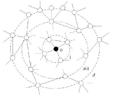
Figure 3: A generic situation in a complex network involving a reference node $i$ (in black) and the respectively defined hierarchical levels. 

Consider the generic situation depicted in Figure 3, including a reference node $i$ and the several respectively defined hierarchical levels, extending from 0 (corresponding to the reference node) to $d$, and further. Recall that the subnetwork $\gamma_{d}(i)$ is the subgraph obtained by considering the $n_{d}(i)$ nodes at level $d$ (i.e. the ring $R_{d}(i)$) and the $e_{d}(i)$ edges among those nodes. It can be shown that the following mean-field recursive approximation holds for a random network with overall mean degree $\left<k\right>$

$$\left\{\begin{array}[]{l}n_{d}(i)\approx\eta(k_{d-1},N-N_{d-1})\\ N_{d}(i)\approx N_{d}(i)+n_{d}(i)\\ k_{d}(i)\approx\left(\frac{N-C_{d}(i)}{N}\right)\left(\sum_{j\in R_{d}(i)}k_{j}\right)n_{d}(i)\end{array}\right.$$ (13)

where $N_{d}(i)$ is the cumulative number of nodes from the hierarchical level 0 up to level $d$ (inclusive), i.e. $N_{d}=\sum_{j=0}^{d}n_{d}(i)$, and the function $\eta(a,b)$ gives the average number of manners $b$ objects can be taken, with repetition, to fill $a$ slots. Now, the average and variance of the hierarchical node degree of node $i$ at distance $d$ can be respectively approximated as

$$E\left[k_{d}(i)\right]\approx\left(\frac{N-N_{d}(i)}{N}\right)\left<k\right>n_{d}(i)$$ (14)

$$Var\left\{k_{d}(i)\right\}\approx\left(\frac{N-N_{d}(i)}{N}\right)^{2}\left<k\right>n_{d}(i)^{2}$$ (15)

Figures 4(a-i) show the hierarchical node degree for several combinations of $\left<k\right>$ and $N$. It is clear from this figure that the hierarchical node degree curves are approximately symmetric with respect to the abscissa $P$ of the respective peak value, which is a consequence of the finite size of the considered networks. Actually, the following three situations can be identified during the dynamic evolution of the hierarchical node degree for a specific network node: (i) the hierarchical node degree increases as more nodes imply links to more nodes; (ii) a peak is achieved with abscissa $P$; and (iii) the node degree decreases because of the finite size of the network, which implies the ‘saturation’ of the hierarchical expansion. Observe also that higher connectivity, implied by large values of $\left<k\right>$, tends to reduce the value of $P$ and, consequently, the hierarchical levels of the networks. Such an effect is usually accompanied by an increase of the heights of the respective curves, in order to conserve the average node degree. As a matter of fact, it can be shown that also important is the fact that the standard deviation tends to increase with the values of the hierarchical node degree.

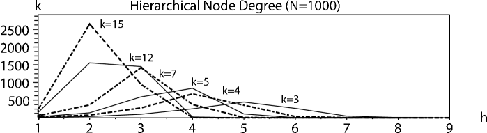
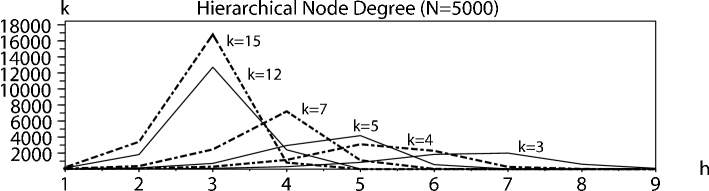
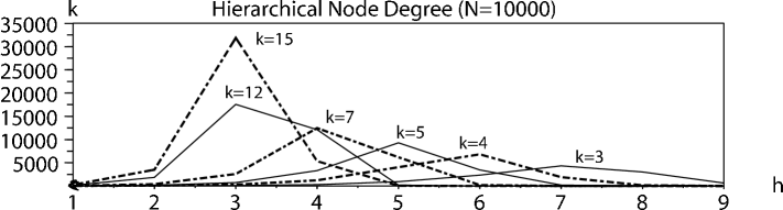
Figure 4: The hierarchical node degree for several configurations of $\left<k\right>$ and $N$. Observe that such curves are always characterized by a peak, which is a consequence if the finite size of the considered networks. Observe also that increased connectivity, implied by larger values of $\left<k\right>$ tends to reduce the number of hierarchical levels in the network. 

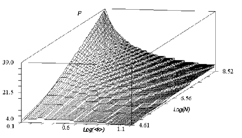
Figure 5: The values of the abscissa of the peak hierarchical node degree for several values of $Log(\left<k\right>)$ and $Log(N)$.  

Figure 5 shows the values of $P$, obtained by simulations using the Equation 15, for several values of $\left<k\right>$ and $N$. Observe that, for a fixed average degree $\left<k\right>$, we have that $P\approx cLog(N)$, for some real constant $c$. It is clear from Figure 5 that the hierarchical levels are much more speedily reduced with the increase of $\left<k\right>$ than with the reduction of $N$, an effect which can also be appreciated from Figure 4.

7 Characterization of Complex Networks Models

In order to further illustrate the potential of the hierarchical measurements discussed so far in this work, they have been used to characterize, through simulations, random, scale-free (i.e. Barabási-Albert – BA) and regular network models.

The random networks are generated by selecting edges with uniform probability $p$. The BA networks are produced as described in [2], i.e. starting with $m0$ randomly interconnected nodes and adding new nodes with $m$ edges which are attached to the existing nodes with probability proportional to their respective node degrees. The considered regular networks are characterized by each node being connected exactly to 8 other nodes. Two types of networks have been studied in this article: one with border effects, where the nodes at its border have a lesser degree; and another without border effects, i.e. considering toroidal connections. In both cases, the nodes are organized into an $L\times L$ array, and each internal node (i.e. non-border node), specified by its position $(x,y)$ in such an array, is connected to its 8-neighbors $(x-1,y)$, $(x+1,y)$, $(x-1,y-1)$, $(x+1,y-1)$, $(x-1,y+1)$, $(x+1,y+1)$, $(x,y-1)$, $(x,y+1)$. The random model assumes $\left<k\right>=15$, $\left<k\right>=5$ and $\left<k\right>=3$, and the BA model considers $\left<k\right>=16$, $\left<k\right>=6$ and $\left<k\right>=4$. These two models assume $N~{}=10000$. In the case of the regular networks, $N=10000$ (i.e. $L=100$) and $\left<k\right>=8$. Observe that the average node degree of the regular network differs from those for the other two models as an unavoidable consequence of the intrinsic topology of that network.

The remainder of this section presents the hierarchical measurements obtained for each of the complex networks types described above. For the sake of comprehensiveness, three instances of each model were considered respectively to decreasing average node degree, namely $k=15$, $5$, and $3$ for Radom Graph Results; $k=16$, $6$, and $4$ for Barabási-Albert model.

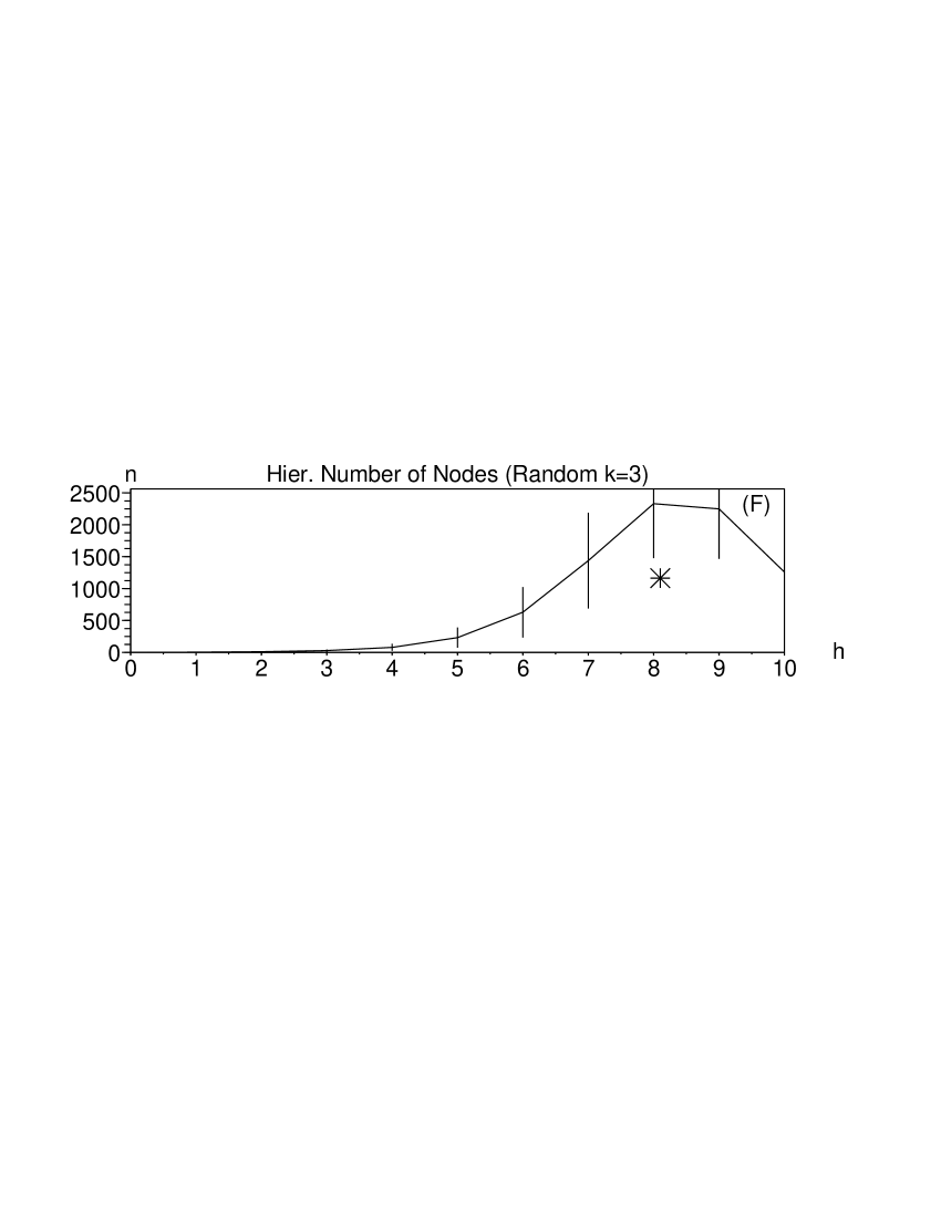
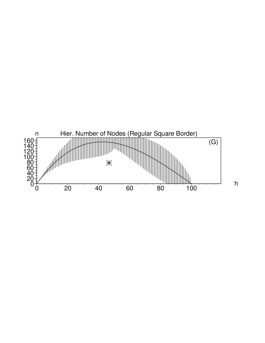
Figure 6: Hierarchical number of nodes (average $\pm$ standard deviation) for all considered networks, which are identified above each graph. Observe that most curves are characterized by a peak. The average value of the shortes path between any two nodes is marked by an asterisk.  

Figure 6 shows the hierarchical number of nodes (average $\pm$ standard deviation) obtained for the considered network models, including three average degree values in the case of the BA and random cases, while taking all nodes into account. The asterisks indicate the position of the average shortest path between any pair of nodes, which are included in order to provide a reference for the hierarchical analysis. All curves are characterized by a peak, except for the regular graph with no border effects. The values of the hierarchical number of nodes obtained for the random models are more susceptible to the change of mean degree (i.e. Figs. 6a-c) than those values obtained for the Barabási-Albert networks. For a decrease from $k=16$ to $k=6$, the peak of the Barabási-Albert model shows a change of only one hierarchical level, while in the Random model, decreasing from $k=15$ to $k=5$, such a displacement involves four levels. For a reduction from $k=5$ to $k=3$ ($k=6$ to $k=4$ for BA), the change was one level for Barabási-Albert, and 3 levels for the random models. This is a direct consequence of the fact that scale-free structures are less susceptible to the removal of random edges (same as reducing the mean degree) than the random models. Hubs in BA model establish shortcuts between nodes, reducing the weight of other edges distances in the average minimal distance. The regular networks without border effects yielded hierarchical number of nodes which are linearly increasing, reflecting the basic structure of such models. However, the regular networks with borders were characterized by a wide peak and high variance of measurements. Interestingly, the peaks obtained for the hierarchical number of nodes occur near the average shortest path marked by the asterisks. Note that the last level with a non-zero value corresponds to the graph diameter [16].

The values of hierarchical node degrees, shown in Figure 7, are similar to the respective measurements of hierarchical number of nodes shown in Figure 6, except for an expected offset of one hierarchical level to the left.

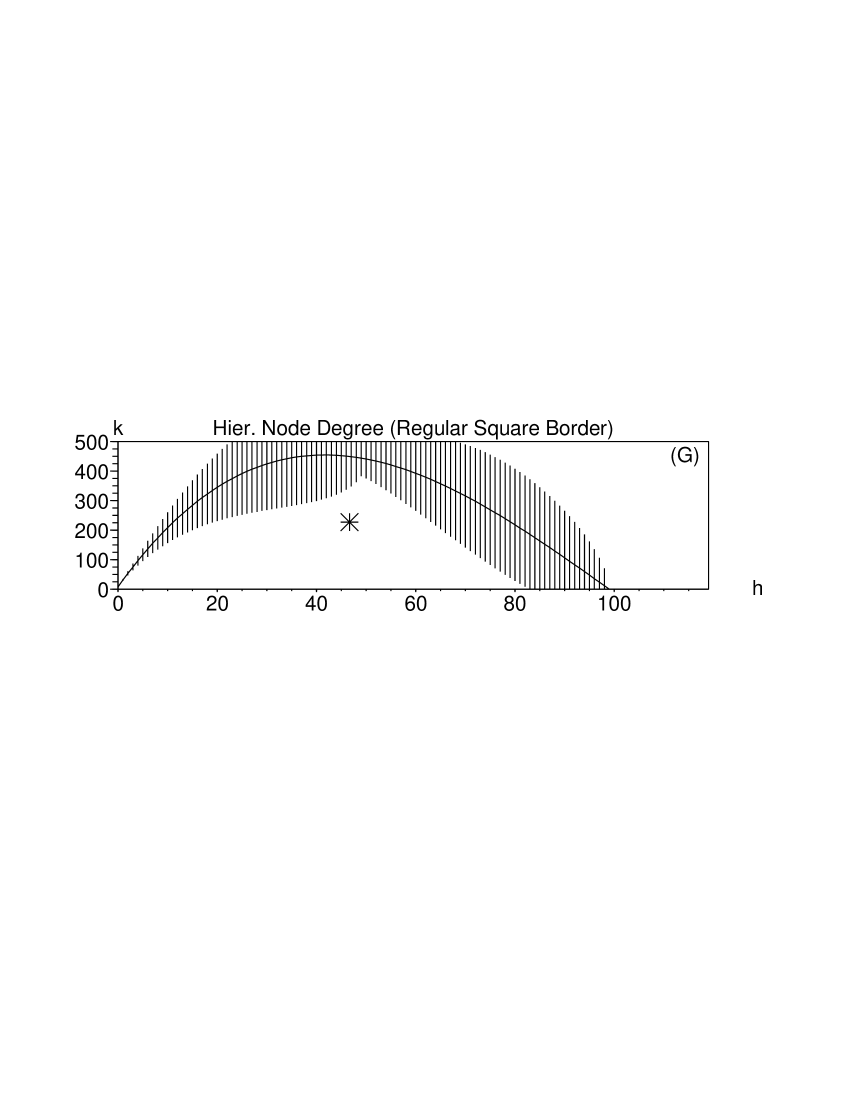
Figure 7: Hierarchical node degrees obtained for all the considered network models. The curves are similar to those obtained for the hierarchical number of nodes, except for a expected offset of one level. 

Figure 8: Inter ring degree values for the considered network models. 

All curves obtained for the inter-ring degree, shown in Figure 8, are monotonically decreasing after the first hierarchical level. Again, the curves obtained for the random networks are less sensitive to variations of the average degree than those obtained for the Barabási-Albert model. The results for the random netwoks show wider and smoother curves, while those obtained for Barabási-Albert tend to be sharper and to concentrate on the left hand side, implying smaller peaks abscissae which are identical for the three considered average degrees. Results obtained for the Barabási-Albert cases also show a peak at the first hierarchical level and present high variance, this is a consequence of the high chance of finding a hub on that level. All models, except for the regular cases, are characterized by presenting the peak of the curve to the left of the asterisk (i.e. the average shortest path). It is also interesting to observe that although this measurement is closely relate to the hierarchical degree, the curves obtained for these two features (i.e. Figures 7 and 8) are markedly different, in the sense that the curves of the hierarchical inter ring degree obtained for the random model no longer presents the peak structure as observed in Figure 7. The curves obtained for the regular networks are also interesting, being characterized by an initial stage of steep decay followed by a plateau which tends to decrease for higher hierarchical levels in the case of the regular network with borders.

Figure 9: Intra Ring Degree values for the considered network models. 

The results for intra-ring degree, shown in Figure 9, are very similar to the hierarchical number of nodes measurement, characterized by a peak, except for regular networks, which exhibit a markedly different evolution resembling the curves obtained for the inter-ring degree. Note that for regular graphs with no border effects, the final decreasing part tends to decrease and saturate. The shape of BA and Random curves are closely similar to those obtained for the hierarchical number of nodes.

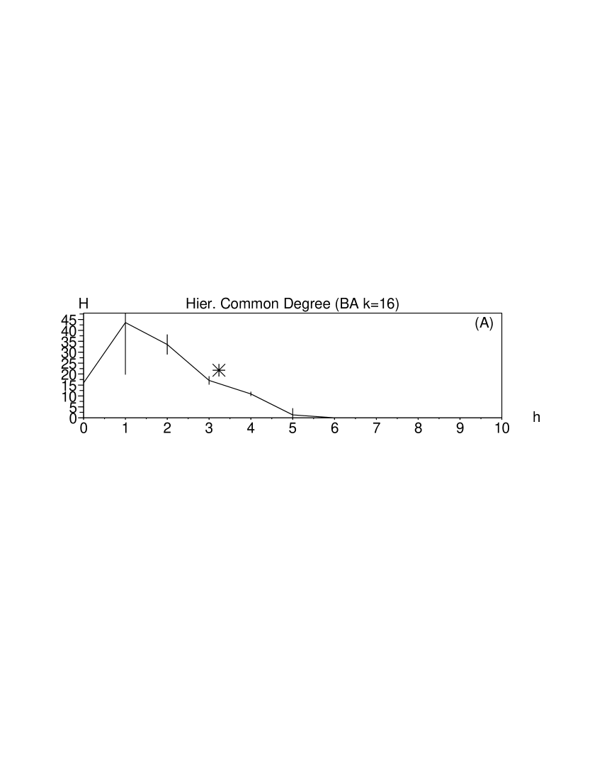
Figure 10: Hierarchical Common Degree measures with the respective $\pm$ standard deviations obtained for the considered models. 

Figure 10 shows the values of hierarchical common degree for the considered network models. These distributions are characterized by a decreasing curve after the first level, excepted for the regular graphs with no border effects. Generally, these curves are similar to those obtained for the inter-ring degrees, except that the present curves are wider. Another observation is that the average hierarchical common degree tends to be higher at the initial hierarchical levels, which is a consequence of the fact that the largest hubs present in the BA model tend to be reached sooner, providing bypasses to the other nodes and therefore reducing the peak abscissae and number of hierarchical levels. This is the main reason why all peaks in the BA networks tend to be displaced to the left hand side than those in the random networks. Like with the other measurements, it can be that the positions of the peaks along the curves are less affected by variations of the average node degree in the cases of the BA models. The curves for random and regular models resulted similar and characterized by an interval of nearly constant values at the intermediate part of the curves. This is a direct consequence of the smaller variance of traditional node degrees in those two models as compared to the higher variance of the BA cases.

Because the regular models have a fixed number of connections for each node, the common degree measurement results in a constant curve with value $k=8$ for the network with border effects. As some nodes (i.e. those at the border) do not have exactly the same degree, the last levels have a smooth decrease but higher standard deviation.

Figure 11: Hierarchical Clustering Coefficient Degree measurements. Note the higher values of standard deviantion relatively to the other measurements. 

The curves of hierarchical clustering coefficients resulted the most distinct among the three considered networks and have the higher standard deviations, as shown in Figure  11. Also involving an intermediate constant interval, the curves obtained for the random models correspond to the smallest clustering coefficients among the models. Therefore, the nodes at each ring of those networks are characterized by low interconnectivity. The hierarchical clustering coefficient curves obtained for the BA case, present much higher values and involve sharper peaks of connectivity, tending to present another peak along the last levels (see Figures 11b-c). The hierarchical clustering coefficient obtained for the regular networks has a monotonically decreasing behavior, with values which start higher than those of the two other considered models. The monotonic decay observed for this case (i.e. regular networks) is explained by the fact that both the number of nodes and edges increase linearly along successive hierarchical levels for that model (see Equation 8). Note that the regular model with and without border are similar.

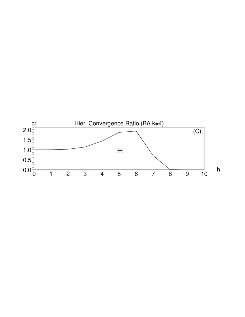
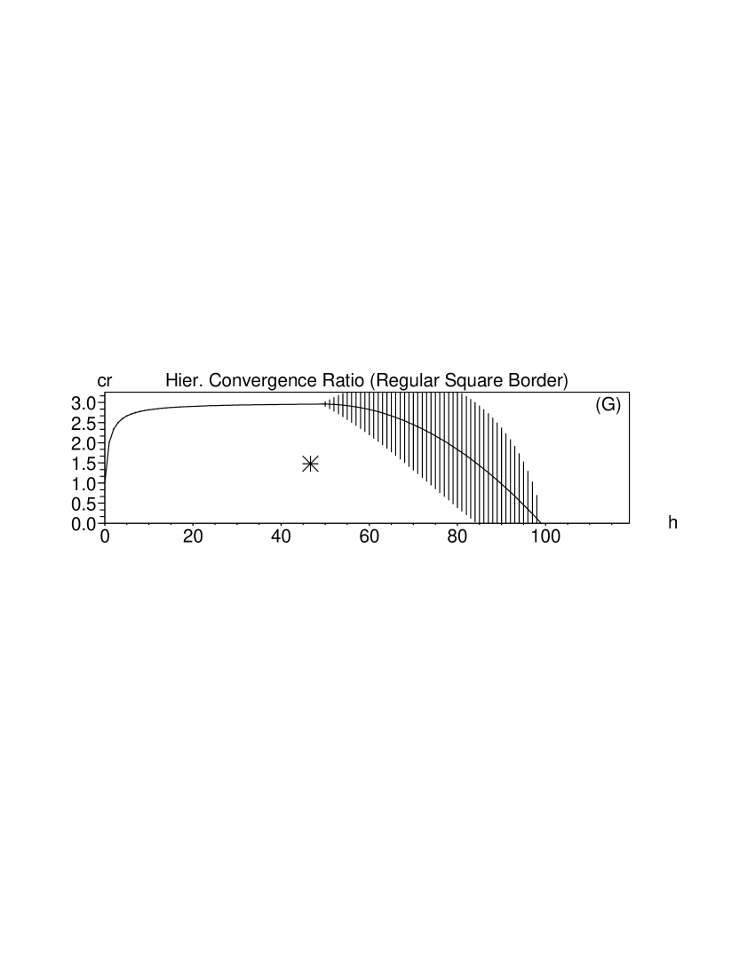
Figure 12: Convergence Ratio measurements for the considered networks. 

The convergence ratios obtained for each of the considered network models are shown in Figure 12. These curves are characterized by similar behavior among themselves with nearly constant value at the first levels and a peak at the last levels (except for the regular models), along which the hierarchical expansion tends to saturate, i.e. after the peak $P$ is reached. Note also that sharper peaks tend to be obtained for high values of $k$. The positions of the peaks are near the average shortest paths.

The convergence ratio curves obtained for the regular networks are also qualitatively similar to those obtained for the other models, but the bordered graphs lack the peak and have a smooth decay along the last levels.

Interestingly, among all considered measurements, it was the hierarchical common degrees and hierarchical clustering coefficients which provided the most distinctive shapes for each respective network model. Therefore, such measurements stand out as particularly promising subsidies for, together with the log-log node degree density, identifying the category of the network under study. Such a possibility is illustrated in the following section.

8 Application to Real Networks

The above described hierarchical measurements have also been applied to characterize three complex networks obtained from real data. These real networks include: a Edinburgh Associative Thesaurus network [39], the 1997 US Airports network ( [40]) and a protein-protein interaction network [31]. The Edinburgh(Word) graph is a empirical association network created as a set of collected words from human subjects who are requested to enter words that first come to their mind after seeing a stimulus word. All the responses are presented with similar frequency. The detailed procedures of the creation of Edinburgh graphs can be seen in [39]. This network has 23219 nodes and $k\simeq 14$ and is oriented and weighted. A similar network has been considered in [36], while a preliminary characterization of such a type of networks by using the hierarchical node degree has been reported in [9]. The protein-protein interaction graph(YEAST), described in  [31], has 2361 nodes with $k\simeq 3$ where a node represents a protein and the edge a interaction between the two respective proteins. The US Airport network is a compilation of flights between the airports of United States in 1997, where a node represents an airport and the edge a flight between the two airports. This network has a total of 332 nodes(airports) and $k\simeq 6.4$. All the considered real graphs were compared to random and BA models with similar node degrees (for the sake of space economy, not all these graphs are shown in Section Characterization of Complex Networks Models).

Figure 13: Hierarchical Number of Nodes obtained for the real networks and considered generated networks. 

Figure 14: Hierarchical Node Degree distribution along hierarchical levels, same results from Number of Nodes.  

The results for the curves of hierarchical number of nodes and node degrees are similar as seen in Figure 13 and 14. Also, no significant differences were observed between these results and those obtained for the respective random or BA simulated networks.

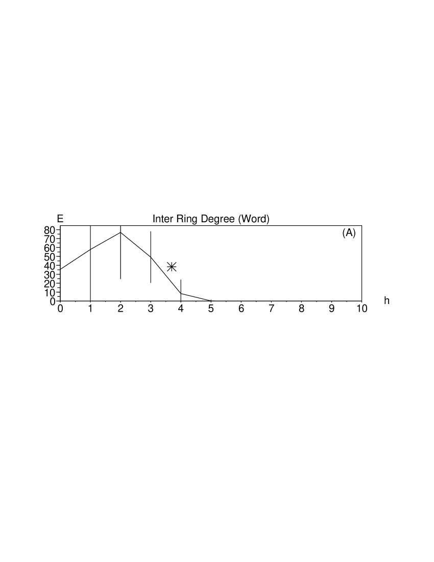
Figure 15: Inter Ring Degree values for real and generated graphs. 

More interesting results have been obtained for the inter-ring degrees, shown in Figure 14. These curves were observed to be more similar to the respective simulated Barabási-Albert curves. In fact, all considered real networks are substantially similar to scale-free networks, being characterized by a high variance of node degrees and the presence of hubs.

Figure 16: Intra Ring Degree measurements obtained for the considered networks. 

The intra ring degrees of the real networks are shown in Figure 16. Interestingly, the curves obtained for the airport (b) and yeast(c) present their respective peaks to the left of the average shortest path (the asterisk position), while in the BA models the peaks tend to coincide with the asterisks as obtained for the word network.

Figure 17: Hierarchical Common Degree Coefficient of real networks. 

Figure 17 shows the measurements of hierarchical common degree. The airport(b) and yeast(c) networks curves have a similar behavior to those obtained for the respective BA curves, with a peak at the first hierarchical level and a decay. However the word network(a) have a mixed behavior, beginning with a increasing curve like in a BA model, but ending with a convex decay like that typically observed in random networks.

Figure 18: Hierarchical Clustering Coefficient measures. 

The clustering coefficient measurements, shown in Figure 18, substantiate the adherence of the real networks with respective BA simulated models. Another interesting result which can be inferred from this figure regards the fact that the hierarchical clustering coefficients are wider and higher for the word (a) than for the respective BA simulations.

Figure 19: Convergence Ratio Degree of real networks. 

Figure 19 shows the convergence ratio measurement values, which yielded the most different curves among the three real networks and among these and the respective models. The curve for the word network (a) is more similar to the BA and random model, being characterized by a low plateau followed by a peak and an abruptly decrease along the last levels. Different curve profiles have been obtained for the airport (b) and yeast curves (c). The yeast curve presents a wider peak, whose position falls near the center of the distribution. The peak of curve obtained for the airport network resulted displaced to the left hand side, far away from the average shortest path. This is a consequence of the fact that, differently of what is obtained for the yeast, the hubs are reached after just a few hierarchical levels while starting from most nodes. Indeed, we have verified experimentally that the position and width of the peak of the convergence ratio is ultimately defined by the distribution of hubs along the hierarchies after starting from individual nodes. Therefore, the relatively narrow peak near the intermediate hierarchical levels obtained for the word network indicates that the hubs in this structure are found, in average, after 3 to 5 hierarchical levels. Although also narrow, the peak of the airport network results in the first levels, where most hubs are concentrated. Finally, the wider peak obtained for the yeast network is a consequence of the fact that the hubs are distributed more evenly along the hierarchical levels.

9 Node Categorization through Hierarchical Clustering

Another possibility for analysis of complex network allowed by the consideration of hierarchical measurements is the classification of individual nodes into similar groups. In order to illustrate such a potential for the characterization of nodes, two complex network are considered, a Barabási-Albert model (generated with $N=332$ nodes and $k\simeq 6$ edges) and the airport network with 332 nodes and $k\simeq 6.4$ edges considered in the last section. This analysis focuses on the clustering coefficient measurement, which is obtained for all nodes of such networks. Only the hierarchical levels up to 5 are considered in this example (the use of additional levels tended to reduce the specificity of the obtained measurements in the case of the real networks considered in this section).

The hierarchical clustering coefficients are calculated as usual and supplied to a hierarchical clustering method [14], namely an agglomerative algorithm, resulting in the trees (also called dendrograms) of measurements shown in figure 20 and figure 21, respectively to the BA and airport networks. For the sake of better visualization, only the four first hierarchical levels are shown in these figures. The x-axes in these two three refer to the similarity between nodes. Starting at the right hand side of the tree, the nodes are merged with basis on the similarity of their hierarchical clustering coefficients, yielding the taxonomical categorization of the nodes into meaningful clusters corresponding to each branching point in the tree. The y-axes express the size the clusters at the third hierarchical level. For instance, the cluster at the top of Figure 20 contains substantially less nodes than the third cluster from the bottom of the figure. bb=0 0 576 164

Figure 20: Dendrogram obtained for the BA model considering the hierarchical clustering coefficients of the nodes up to hierarchical level 5. Starting from the righthand side of the tree, the nodes are progressively merged into clusters in terms of their similarity. 

Figure 21: Dendrogram obtained for the airport network considering the hierarchical clustering coefficients of the nodes up to hierarchical level 5. 

Figures 22 and 23 show the graphs of average $\pm$ standard deviation of the hierarchical clustering coefficients obtained at each respective level in the dendrograms. The mean degree and percentage of nodes with respect to the whole network for each cluster are given above each graph. Unlike the dendrograms in Figures 20 and 21, the x-axes of the trees in Figures 22 and 23 do not consider the level of similarity between the groups, which is done for the sake of better visualization of the graphs obtained for each cluster of nodes. Starting from the whole network cluster at the right-hand side of the tree, we can observe the progressive division of the node hierarchical signatures in terms of subclasses sharing the basic patterns of hierarchical clustering coefficient shown in the respective graphs. Such a taxonomical characterization of the nodes into subclasses provides substantially more discrimination and characterization than the graphs of average $\pm$ standard deviation obtained considering the whole network such as those discussed in the previous section. This enhanced potential of node discrimination and characterization provided by the dendrograms are particularly useful in the case of networks exhibiting the small world property, as such cases tend to produce hierarchical signatures extending over relatively few hierarchical levels.

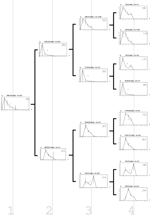
Figure 22: Graphs of the average $\pm$ standard deviation of the hierarchical clustering coefficient obtained for the BA model. Each graph corresponds to the clusters of nodes obtained in the four first hierarchical levels of the dendrogram in Figure 20. 

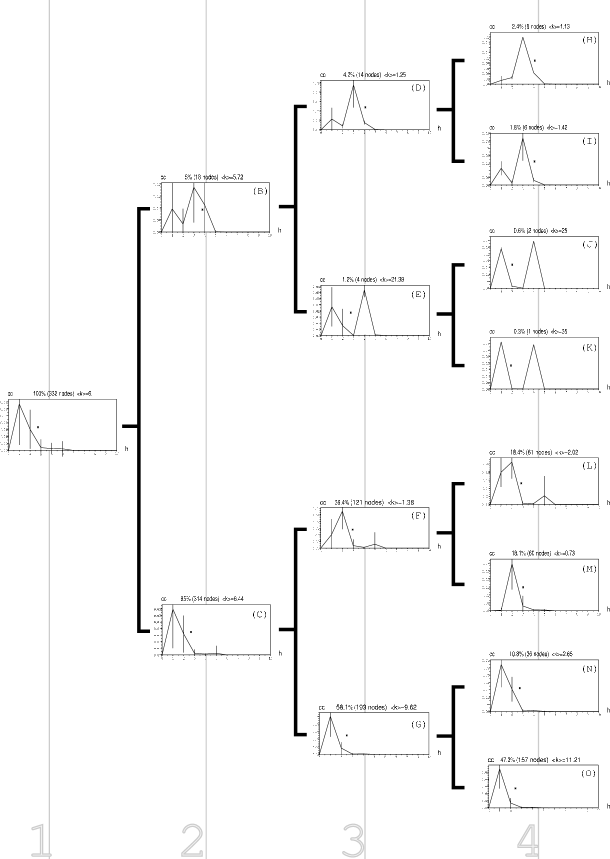
Figure 23: Graphs of the average $\pm$ standard deviation of the hierarchical clustering coefficient obtained for the airport network. 

10 Concluding Remarks

This article has addressed, in a didactic and comprehensive fashion, how a set of hierarchical measurements can be used for the characterization of important topological properties of complex networks. Motivated by the concept of extended neighborhoods and distances, the identification of hierarchical levels along the network, with reference to each of its nodes, allows the definition of a series of useful and informative hierarchical measurements of the network topology, including hierarchical extensions of the traditional node degree and clustering coefficient measurements. The novel concepts of inter and intra-ring degrees, convergence ratio, edge degree and edge clustering coefficient, as well as their hierarchical versions, were also introduced here in terms of the subnetwork generalization described in [10].

It has been shown, both analytically and through simulations, that the hierarchical node degree of a random network has a typical shape involving a limited number of hierarchical levels while a peak is observed at its intermediate portion, which is a consequence of the finite size of the considered networks. A similar dynamics was experimentally identified for scale-free and regular network models. It was also shown, through simulations, that the suggested set of hierarchical measurements provided a wealthy of information about the topological structure of the considered models (namely random, scale-free and regular), allowing the identification of a number of interesting properties specific to each of those models. Of particular interest is the discriminative potential of the hierarchical common degree and hierarchical clustering coefficient. The potential of the reported set of hierarchical measurements was further illustrated with respect to three real networks: word associations, airport connections and protein-protein interactions. The comparison of the hierarchical measurements obtained for these three networks with respective random, regular and BA models with the same number of nodes and similar node degree indicated that, except for a few measurements (specific to each model), all the three real networks were most similar to the BA models. In the case of the word associations network, some measurements (i.e. hierarchical common degree and inter-ring degree) yielded hierarchical curves which were similar to random along some parts and similar to BA at other parts. This network was also verified to present the convergence ratio most similar to that of a respective BA model. The concentration of higher values of convergence ratio at the left hand side of the curves obtained for the airport network also confirmed the fact that the hubs in this network are reached much faster than all the other networks considered in this article. Contrariwise, the convergence ratio values obtained for the protein-protein interaction network indicated that the hubs in this real network are more evenly spaces one another. As a matter of fact, the convergence ratio resulted in the most informative of the hierarchical measurements as far as the analysis of the three real models was concerned. This is a consequence of the fact that the presence of a hub at a given hierarchical level tend to strongly affect the convergence ratio at that level.

Finally, the current article also proposed and illustrated the possibility to use the enhanced information provided by the set of hierarchical measurements in order to organize the nodes of a network into a taxonomy reflecting the similarities between the nodes connectivity. Such a methodology is particularly promising because the obtained taxonomy can be used to better understand the main classes of nodes present in a given complex network, i.e. those classes obtained at the higher levels of the taxonomy. Indeed, while the limited number of hierarchical levels present in small world networks such as random and BA models constrain the potential of the hierarchical measurements for the discrimination between such models, the consideration of the main obtained classes of nodes has been verified to provide further discrimination between the compared networks.

A series of possible future investigations has been motivated by the results reported in this article. First, it would be interesting to assess in a systematic fashion, and by using multivariate statistical analysis and hypothesis tests, the potential of each measurement, as well as their combinations, for discriminating the possible class of a given network. Another issue of particular relevance regards the identification and preservation of hubs considering not only the immediate neighbors of a node, but of the neighbors accumulated along growing hierarchical levels. While such a possibility has been preliminary considered in [10], it would be interesting to consider the preservation of hubs as an increasing number of hierarchical levels is taken into account. Such a study is under development with respect to protein-protein association networks and related results should be futurely presented. Another study which can complement the results described in the current work involves the consideration of several types of small-world networks. Finally, it would be interesting to apply the hierarchical measurements for the characterization of several other real networks such as protein-protein interaction, internet, social connections, to name but a few.

Acknowledgment: Luciano da F. Costa is grateful to FAPESP (proc. 99/12765-2), CNPq (proc. 308231/03-1) and the Human Frontier Science Program (RGP39/2002) for financial support.

References

- [1] M.E.J. Newman, SIAM Review 45: 167–256 (2003).
- [2] R. Albert and A.-L. Barabási, Rev. Mod. Phys. 74: 47–97 (2002).
- [3] P.J. Flory, J. Am. Chem. Soc 63: 3083, 3091, 3096 (1941).
- [4] A. Rapoport, Bull. Math. Bioph. 19: 257–277 (1957).
- [5] P. Erdös and A. Rényi, Publications Mathematicae 6: 290-297 (1959).
- [6] D.J Watts and S.H. Strogatz, Nature 393: 440–442 (1998).
- [7] D.J. Watts, Small Worlds, Princeton Studies in Complexity, Princeton Univ. Press (1999).
- [8] R. Albert and H. Jeong and A.L. Barabási, Nature 401: 130, cond-mat/9907038 (1999).
- [9] L.daF. Costa, Phys. Rev. Lett. 93: 098702 (2004).
- [10] L.daF. Costa, cond-mat/0408076 (2004).
- [11] E. Ravasz and A.L. Barabási, cond-mat/0206130 (2002).
- [12] E. Ravasz, A.L. Somera, A. Mongru, Z.N.Oltvai and A.L. Barabási, Science, 297: 1551–1555 (2002), cond-mat/0209244.
- [13] G. Caldarelli, R. Pastor-Satorras and A. Vespignani, cond-mat/0212026 (2003).
- [14] Costa, L. d. and Cesar, R. M. 2000, Shape Analysis and Classification: Theory and Practice, 1st. CRC Press, Inc.
- [15] R. Duda, P. Hart, and D. Stork: Pattern Classification, 2st. John Wiley, New York, 2001.
- [16] B. Bollobás. Random Graphs. Academic Press, London, 1985.
- [17] A.L Barabási, Z. Deszo, E. Ravasz, S.-H. Yook and Z. Oltvai, Sitges Proceedings on Complex Networks (2004).
- [18] A Trusina, S. Maslov, P. Minnhagen and K. Sneppen, Phys. Rev. Lett., 92: 178702 (2004), cond-mat/0308339 (2003).
- [19] M. Boss, H. Elsinger, M. Summer and S. Thurner, Santa Fe Institute Working Paper No. 03-10-054, Accepted for Quant. Finance, cond-mat/0309582 (2003).
- [20] M. Barthélemy, A. Barrat, R. Pastor-Satorras and A. Vespignani, cond-mat/0311501 (2003).
- [21] H. Zhou, Phys. Rev. E, 67: 061901 (2003).
- [22] A. Vázquez, Phys. Rev. E, 67: 056104 (2003).
- [23] M. Steyvers and J.B. Tenenbaum, To appear in Cognitive Science, cond-mat/0212026 (2003).
- [24] V. Gold’shtein, G.A. Koganov and G.I. Surdutovich, cond-mat/0409298 (2004).
- [25] E.R. Dougherty and R.A. Lotufo, Hands-on Morphological Image Processing, SPIE Press (2003).
- [26] M. E. Newman, cond-mat/0111070 (2001).
- [27] M. E. J. Newman and D. J. Watts, Phys. Rev. E 60, 7332-7342 (1999).
- [28] R. Cohen, S. Havlin, S. Mokryn, D. Dolev, T. Kalisky, and Y. Shavitt, cond-mat/0305582(2003).
- [29] L. Vincent, Signal Proc., 16:365–388 (1989).
- [30] H.J.A.M. Heijmans, P. Nacken, A. Toet and L. Vincent, J. Vis. Comm. and Image Repr., 3:24–38 (1992).
- [31] Shiwei Sun, Lunjiang Ling, Nan Zhang, Guojie Li and Runsheng Chen: Topological structure analysis of the protein-protein interaction network in budding yeast. Nucleic Acids Research, 2003, Vol. 31, No. 9 2443-2450.
- [32] L.daF. Costa, cond-mat/0405022 (2004).
- [33] J.P. Bagrow and E.M. Bollt, cond-mat/0412482 (2004).
- [34] A.C. Zorach and R.E. Ulanowicz, Complexity, 8(3): 68–76 (2003).
- [35] T.H. Cormen, C.E. Leiserson, R.L. Rivest and C. Stein, Introduction to Algorithms, The MIT Press (2002).
- [36] L.daF. Costa, Intl. J. Mod. Phys. C, 15:371–379 (2003).
- [37] L.daF. Costa, q.bio.MN/0405028 (2004).
- [38] L.daF. Costa, q.bio.TO/0412042 (2004).
- [39] Kiss, G.R., Armstrong, C., Milroy, R., and Piper, J. (1973) An associative thesaurus of English and its computer analysis In Aitken, A.J., Bailey, R.W. and Hamilton-Smith, N. (Eds.), The Computer and Literary Studies. Edinburgh: University Press.
- [40] USAir97, Pajek Package for Large Network Analysis http://vlado.fmf.uni-lj.si/pub/networks/pajek/data/gphs.htm