Long range polarization attraction between two different likely charged macroions

Abstract

It is known that in a water solution with multivalent counterions ($Z$-ions) two likely charged macroions can attract each other due to correlations of $Z$-ions adsorbed on their surfaces. This “correlation” attraction is short-ranged and decays exponentially with increasing distance between macroions at characteristic distance $A/2\pi$, where $A$ is the average distance between $Z$-ions on the surfaces of macroions. In this work, we show that an additional long range “polarization” attraction exists when the bare surface charge densities of the two macroions have the same sign, but are different in absolute values. The key idea is that with adsorbed $Z$-ions, two insulating macroions can be considered as conductors with fixed but different electric potentials. Each potential is determined by the difference between the entropic bulk chemical potential of a $Z$-ion and its correlation chemical potential at the surface of the macroion determined by its bare surface charge density. When the two macroions are close enough, they get polarized in such a way that their adjacent spots form a charged capacitor, which leads to attraction. In a salt free solution this polarization attractive force is long ranged: it decays as a power of the distance between the surfaces of two macroions, $d$. The polarization force decays slower than the van der Waals attraction and therefore is much larger than it in a large range of distances. In the presence of large amount of monovalent salt, the polarization attraction decays exponentially at $d$ larger than the Debye-Hückel screening radius $r_{s}$. Still, when $A/2\pi\ll d\ll r_{s}$, this force is much stronger than the van der Waals attraction and the correlation attraction mentioned above. The recent atomic force experiment has shown some evidence for this polarization attraction.

I Introduction

Water solutions of strongly charged colloidal particles (macroions) with multivalent ($Z$ valent) counterions ($Z$-ions) are important in physics, chemistry, biology and chemical engineering. Colloidal particles, charged lipid membranes, DNA, actin, and even cells and viruses are examples of different macroions. Multivalent metallic ions, dendrimers, charged micelles, short DNA and other relatively short polyelectrolytes like spermine can play the role of $Z$-ions. Several interesting, counterintuitive phenomena have been discovered in such a system, such as charge inversion, which have attracted significant attention (see review paper Ref. Nguyen-review and references therein). Charge inversion happens in a water solution when a macroion binds so many $Z$-ions that its net charge changes sign. This phenomenon is especially important for gene therapy. To deliver DNA into the cell, charge of negative DNA (playing the role of macroion) should be inverted by positive $Z$-ions to approach a negatively charged cell membrane. Here we actually assume that the membrane is weakly charged and therefore its charge is not inverted. The question is what happens if the charge of the membrane is also inverted by positive $Z$-ions. Can DNA still be attracted to the membrane?

A similar question was put forward by the recent atomic force experimentLemay designed to verify the theory of charge inversion based on strong correlations between $Z$-ions Boris ,Nguyen-review In the experiment, forces between a negatively charged spherical macroion attached to the cantilever (probe) and a positively charged surface were measured at different concentrations of positive $Z$-ions (see Fig. 1a) Lemay . At small concentrations of $Z$-ions, the probe is attracted to the surface. With increasing concentration of $Z$-ions, the charge of the probe gets inverted by $Z$-ions, and the measured force at large $d$ becomes repulsive, where $d$ is the distance of closest proximity from the probe to the surface. The critical concentration of $Z$-ions, where this happens is in reasonable agreement with the prediction of Ref. Boris . However, an interesting new feature of the repulsive force was observed. With decreasing $d$, the repulsive force reaches a maximum at $d\simeq 100$ $\AA$ (which is roughly equal to the Debye-Hückel screening radius of the solution) and start to decrease. This suggests the existence of a competing attraction.

One can also consider a different experimental setup Sivan in which the probe and the surface are likely charged and both adsorb $Z$-ions (Fig. 1b). When the concentration of $Z$-ions is high enough so that the charges of the surface and the probe are both inverted at large $d$, it is interesting to find out whether the force may be attractive. Preliminary experiments showed such attraction  Sivan . Notice that this setup brings us back to the original question of attraction of charge-inverted DNA to charge-inverted cell membrane.

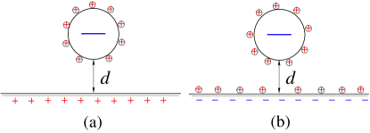
Figure 1: Schematic illustration of two experimental setups for atomic force measurements of likely charged macroions. The force between the probe (the big sphere with negative charge) and the surface is measured at different concentrations of $Z$-ions (small spheres with positive charges). (a) In the setup of Ref. Lemay , the bare surface and the bare probe are the oppositely charged so that positive $Z$-ions are only adsorbed to the probe and invert its charge. (b) In the setup of Ref. Sivan , the bare surface and the bare probe are likely charged so that positive $Z$-ions are adsorbed to both of them, again making them likely charged at large $d$.

Motivated by these questions, in this paper we study the interaction between two different macroions in the presence of a large concentration of $Z$-ions. In the main part of the paper, we focus on the case of two bare negatively charged macroions and positive $Z$-ions corresponding to Fig. 1b, since it is pedagogically simple. Only in Sec. V, we discuss the case of oppositely bare charged macroions (Fig. 1a) in the connection with Ref. Lemay . We assume that the valence of $Z$-ions, $Z\gg 1$, but still many $Z$-ions are needed to neutralize one macroion. The two macroions are spherical but different in their bare surface charge densities. We will see that this is crucial to produce the attraction. Actually this is the reason why this attraction was not reported before, when the focus was on identical macroions Nguyen-review . In calculation, we focus on the two limiting cases, $R_{1}=R_{2}$ and $R_{1}\ll R_{2}$, where $R_{1}$ and $R_{2}$ are the radii of the two macroions.

Figure 2: $Z$-ions are strongly correlated on the surface of the macroion. Their short range order is similar to that of a Wigner crystal with lattice constant $A$.

Before we discuss the mechanism of this attraction, let us first briefly review the theory of charge inversion Boris . Let us consider a water solution with one negatively charged macroion and many positively charged $Z$-ions. Due to the Coulomb interaction, $Z$-ions are adsorbed to the surface of the macroion. On the surface, they strongly repel each other with energy much larger than $k_{B}T$ and form a two dimensional strongly correlated liquid with short range order similar to a Wigner crystal (WC) (Fig. 2). When a new $Z$-ion approaches the macroion, it repels already adsorbed $Z$-ions and creates a negative spot for itself. One can view it as an electrostatic image of the $Z$-ion, similar to the image on a conventional conducting surface. Attraction to the image leads to an additional negative chemical potential $\mu_{c}$ ($c$ stands for “correlation”) for each $Z$-ion on the surface of the macroion. As a result, when the concentration of $Z$-ions in the solution is large enough, so many $Z$-ions are adsorbed that the net charge of the macroion is inverted and becomes positive Boris .

As pointed out in Ref. Boris , for an already neutral macroion, adsorption of additional $Z$-ions can be viewed as charging a conductor of certain capacitance with a fixed electric potential $\phi$. This potential is determined by the difference between the chemical potential of $Z$-ions in the solution and the correlation chemical potential $\mu_{c}$ on the surface. It is a constant all over the macroion surface because the net surface charge density of the macroion changes very little and therefore $\mu_{c}$ is a constant (see Sec. II for detail discussion). Actually, this electric potential is similar to the surface potential of a colloidal particle determined by its “potential-determining ions” given by the Nernst equation Colloid . The only difference is that in the present case, $\mu_{c}$ originates from correlations of $Z$-ions instead of chemical bonding.

The model of conductors is convenient to discuss the interaction and understand the possible attraction between two different macroions in the presence of $Z$-ions. Actually, as we know from electrostatics, if two conductors are charged with different potentials, they may attract each other, even though the two potentials have the same sign. For example, consider two conducting spheres 1 and 2 with same size and potentials $\phi_{1}$ and $\phi_{2}$ respectively and $\phi_{1}>\phi_{2}>0$. When the two spheres are far away, they repel each other. When we bring them closer, adjacent spots of two spheres form a charged capacitor with potential difference $\phi_{1}-\phi_{2}$. In other words, spheres get polarized. The polarization attraction competes with the overall repulsion between two spheres (since $q_{1}>q_{2}>0$) and dominates at small distances between spheres. Similar polarization leads to attraction of a conducting sphere to a close conducting plate holding at different potentials.

Using the model of conductors, we find that as long as the bare surface charge densities of the two macroions are different, they always attract each other at small enough distances, even when their bare charges or net charges are of the same sign. This polarization attraction is even more appreciable in the case that the sizes of the two macroions are very different as in Fig. 1. We also find that the attractive polarization force $F_{p}$ decays with increasing distance as a power law. In the case of Fig. 1, at $d\ll r_{s}$, we get

$$F_{p}=-\frac{\pi DR_{1}}{d}(\phi_{1}-\phi_{2})^{2},$$ (1)

where $r_{s}$ is the Debye-Hückel screening radius, $D=80$ is the dielectric constant of water and $R_{1}$ is the radius of the spherical probe.

We emphasize that the polarization attraction discussed here is different from two standard attractive forces. The first one is the well known van der Waals attraction used in standard DLVO theory Colloid . In the case of Fig. 1, it is given by

$$F_{vdW}=-\frac{R_{1}H}{6d^{2}},$$ (2)

where $H$ is the Hamaker constant. It is clear that $F_{vdW}$ decays with $d$ faster than $F_{p}$. The ratio of these two forces is

$$\frac{F_{p}}{F_{vdW}}=\frac{6\pi Dd}{H}(\phi_{1}-\phi_{2})^{2}.$$ (3)

For the typical $H=1.0\times 10^{-20}J=2.4k_{B}T$ and reasonable $|\phi_{1}-\phi_{2}|\simeq 0.4k_{B}T/e$ (see Sec. II), this ratio is larger than unity if $d>6$ $\AA$.

The second competing force is the short range attraction between two macroions due to correlations of $Z$-ions on their surfaces Bloomfield . In the spot where two macroions touch each other, the surface density of $Z$-ions is doubled and the correlation energy is gained. This correlation attraction is related to Wigner-crystal-like arrangement of $Z$-ions on the surfaces and therefore decays exponentially with increasing distance as $e^{-2\pi d/A}$, where $A$ is the “lattice constant” of the Wigner crystal (see Fig. 2). For $d\gg A/2\pi$, it becomes much weaker than the polarization attraction given by Eq. (1) (we assume that $r_{s}\gg A/2\pi$). In this sense the polarization attraction is a long range force.

One can understand the polarization attraction from another point of view, i.e., from the concept of contact electrification. As well known, when two different solids contact to each other in vacuum, due to the difference in their work functions, certain amount of electrons move from one material to the other, developing a electric voltage which stops further charging. This contact electrification leads to the well known Coulomb attraction between them Landau . Here a contact between two objects is necessary to eliminate the kinetic barrier for electrons and makes electrification possible during time of experiments. If we wait long enough, the electrification can happen even without a close contact. In our case of macroions in water, $Z$-ions play the role of electrons and the absolute value of chemical potential $\mu_{c}$ of a $Z$-ion on the surface of the macroion plays the role of the work function. To keep the same electro-chemical potential of $Z$-ions, since $\mu_{c}$ is different for two macroions, the electric potentials must also be different, which leads to attraction. The difference in our system is that the kinetic barrier for $Z$-ions is relatively small and the equilibrium of $Z$-ions is easily achieved through the solution.

Similar electrification phenomenon has been studied in Ref. Messina in a toy model of two negative spherical macroions exactly neutralized by $Z$-ions. The two spheres had the same radius, but substantially different bare charges. It was shown that under conditions of total neutrality one sphere becomes undercharged (negative) and the other is overcharged (positive) and, therefore, they attract each other.

In the present paper, we discuss a more generic and realistic situation: there is certain concentration of $Z$-ions in the solution (a fixed chemical potential of Z-ions) and the macroions can be both either undercharged or overcharged by them. In spite of the same sign of their net charges these macroions attract each other at small distances because of local polarization around the points of closest proximity.

In the presence of large amount of monovalent salt, the Coulomb interaction is effectively truncated at the Debye-Hückel screening radius $r_{s}$. When $\phi_{1}=\phi_{2}$, the two macroions with adsorbed $Z$-ions repel each other as described by the standard DLVO theory Colloid . However, when $\phi_{1}\neq\phi_{2}$, i.e., when the two macroions are different, the polarization attraction appears. When $\phi_{1}$ and $\phi_{2}$ have the same sign, it decays as $e^{-2d/r_{s}}$ at distances larger than $r_{s}$. Still, for $A/\pi\ll d\ll r_{s}$, this attraction is much stronger than both the van der Waals attraction Colloid and the correlation attraction Bloomfield , which is proportional to $e^{-2\pi d/A}$.

This paper is organized as follows. In Sec. II, we describe the interaction between two different macroions in the presence of $Z$-ions and show that it is similar to the interaction between two conductors with different potentials. In Sec. III, we discuss the interaction of two conducting spheres and derive the power law of the attractive force. In Sec. IV, we take into account of the effect of screening by monovalent salt. In Sec. V, we generalize our theory to the case when only one macroion adsorbs $Z$-ions in the connection with the experiment in Ref. Lemay (see Fig. 1a). We conclude in Sec. VI.

II The model of conductors for two macroions in the presence of $Z$-ions

In this section we show that the interaction between two macroions in the presence of $Z$-ions can be considered as the interaction between conductors with different electric potentials. Let us first consider a single spherical macroion with radius $R$ and bare charge $-Q<0$ in a water solution with $Z$-ion concentration $n$. The bare surface charge density of the macroion is $-\sigma=-Q/4\pi R^{2}$. As we discussed in Sec. I, $Z$-ions on the surface of the macroion strongly repel each other to form a strong correlated liquid, similar to a structure of Wigner crystal in the short range (see Fig. 2). The chemical potential related to this correlation is dominated by its low temperature expression, which can be estimated from the Coulomb interaction inside each WC cell (see Eq. (9) in Ref. Boris for the full finite temperature expression of $\mu_{c}$)

$$\mu_{c}(s)\simeq-\frac{1.65Z^{2}e^{2}}{Dr}=-\frac{1.65\sqrt{\pi s}Z^{2}e^{2}}{D}.$$ (4)

Here $s$ is the surface density of $Z$-ions on the macroion, and $r=A\sqrt{\sqrt{3}/2\pi}$ is the radius of the WC cell (see Fig. 2). It satisfies $\pi r^{2}s=1$.

The equilibrium condition of a $Z$-ion in the solution then reads

$$\frac{ZeQ^{\ast}}{DR}+\mu_{c}(s)=-k_{B}T\ln\left(\frac{s^{3/2}}{n}\right),$$ (5)

where $Q^{\ast}$ is the net charge of the macroion combined with adsorbed $Z$-ions. The left hand side is the electrostatic energy of a $Z$-ion at the surface of the macroion plus the correlation chemical potential. The right hand side is the difference between the entropic parts of the chemical potentials of a $Z$-ion in the solution and at the surface. As we will see below, this equilibrium condition is the key for the analogy with conductors.

When $n$ increases, the number of $Z$-ions adsorbed to the macroion also increases. At some critical $n=n_{0}$, $Q^{\ast}$ becomes zero. According to Eq. (5), we have

$$n_{0}=s_{0}^{3/2}\exp\left(\frac{-|\mu_{c}(s_{0})|}{k_{B}T}\right).$$ (6)

Here $s_{0}=\sigma/Ze$ is the surface density of $Z$-ions to neutralize the macroion. The corresponding radius of WC cell is $r_{0}$. In the case we are interested, $\mu(s_{0})\simeq Z^{2}e^{2}/Dr_{0}\gg k_{B}T$ (this defines “strongly charged” $Z$-ions). Therefore $n_{0}$ is an exponentially small concentration which is easy to reach in experiments. For $n>n_{0}$, more $Z$-ions come to the macroion and $Q^{\ast}$ becomes positive. According to Eq. (5), when $n$ is so large that the entropy term is completely negligible, the maximum value of inverted $Q^{\ast}$, $Q_{max}^{\ast}$, is achieved Boris ,

$$Q^{\ast}_{max}=0.8\sqrt{QZe}.$$ (7)

It is calculated by assuming

$$s\simeq s_{0},\ \ \mu_{c}(s)\simeq\mu_{c}(s_{0}).$$ (8)

This assumption is self-consistent, since for $Q\gg Ze$ we have $(s_{max}-s_{0})/s_{0}=Q_{max}^{\ast}/Q=0.8\sqrt{Ze/Q}\ll 1$.

Now we can clearly see the similarity between a neutralized macroion and a neutral conductor. For a given $n>n_{0}$, the charging process from $Q^{\ast}=0$ to $Q^{\ast}>0$ can be viewed as charging a conductor with fixed potential. Indeed, the equilibrium condition Eq. (5) can be written as

$$Q^{\ast}=DR\phi,$$ (9)

with

$$\phi=\frac{|\mu_{c}(s_{0})|-k_{B}T\ln(s_{0}^{3/2}/n)}{Ze}.$$ (10)

Notice that $\phi$ can be expressed through $s_{0}$ because of Eq. (8). Eq. (9) is exactly the same as the expression of charge for a conductor with capacitance $C=DR$ and charged at fixed potential $\phi$. For $n<n_{0}$, by similar discussion, we have a conductor charged at $\phi<0$, providing that $|Q^{\ast}(n)|\ll Q$ so that Eq. (8) is still satisfied.

Now let us consider two macroions in a water solution with $Z$-ions. Clearly, when $d$ is very large, if $n$ is close to $n_{0}$ for both macroions, the analogy to conductors holds. The two macroions have electric potentials $\phi_{1}$ and $\phi_{2}$. When $d$ decreases, due to the interaction between two macroions, $s$ changes and becomes nonuniform on their surfaces. When $d$ is very small, $s$ may become substantially different from $s_{0}$ at closest spots of the two surfaces. Then Eq. (8) is not valid and $\phi_{1,2}$ start to change with $d$ potential . In this paper, we stay in the limit of large $s_{0}$ so that $|s-s_{0}|\ll s_{0}$. Accordingly, Eq. (8) is always valid and our approximation of fixed potentials is fine.

Rewriting Eq. (10) for two macroions, we have

$$\phi_{1,2}=\frac{|\mu_{c}(s_{1,2})|-k_{B}T\ln(s_{1,2}^{3/2}/n)}{Ze}.$$ (11)

Here the subindexes $1,2$ represent two macroions respectively. $s_{1,2}$ are the number densities of $Z$-ions which neutralize two macroions, i.e., $s_{1,2}=\sigma_{1,2}/Ze$. Notice that $\phi_{1,2}$ are completely determined by $n$ and $s_{1,2}$, i.e., the concentration of $Z$-ions and the bare surface charge densities of the two macroions. For a given solution of $Z$-ion concentration $n$, if $\sigma_{1}\neq\sigma_{2}$, $\phi_{1}\neq\phi_{2}$. For example, for typical values $Z=+3$, $n=1$ mM, $-\sigma_{1}=-0.75$ e/nm² and $-\sigma_{2}=-0.45$ e/nm², we have $\phi_{1}=0.77k_{B}T/e$, $\phi_{2}=0.37k_{B}T/e$ and $|\phi_{1}-\phi_{2}|=0.40k_{B}T/e$. Here $\mu_{c}(s_{1})=-7.6k_{B}T$ and $\mu_{c}(s_{2})=-5.7k_{B}T$ are calculated using the full expression of $\mu_{c}$ given by Eq. (9) in Ref. Boris .

In order to calculate the force between two macroions, we can imagine that they are conductors in ion-free water with potentials $\phi_{1}$ and $\phi_{2}$ supported by two batteries. Such conductors are not in equilibrium with each other while our macroions are in equilibrium. This however does not matter for the calculation of the force which is the same in both cases. Indeed, the force depends only on potentials and capacitance matrix of the system.

III Attraction of two conducting spheres with different potentials

In this section, let us focus on the interaction of two conducting spheres 1 and 2 with radii $R_{1}$ and $R_{2}$ and potentials $\phi_{1}$ and $\phi_{2}$ in ion-free water (see Fig. 3). As we explained in the previous section, this interaction is equivalent to the interaction between macroions covered by $Z$-ions. We define the the distance of closest proximity between the two spheres as $d$ and the distance between the centers of the two spheres as $L=d+R_{1}+R_{2}$ (see Fig. 3). Below we use $L$ or $d$ alternatively for convenience. We focus on two limiting cases when $R_{1}=R_{2}$ and $R_{1}\ll R_{2}$, but our approach is applicable for any two spheres.

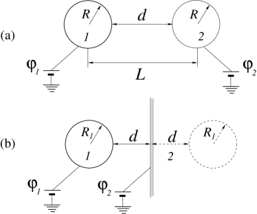
Figure 3: The interaction between two spherical macroions in the presence of $Z$-ions can be considered as the interaction between two conducting spheres with fixed but different electric potentials. We focus on two cases: (a) The size of the two spheres are equal. (b) The size of sphere 2 is much larger than sphere 1 (the radius of sphere 2, $R_{2}$, is not shown). For $d\ll R_{2}$, the interaction between two spheres can be considered as the interaction between sphere 1 with its “image sphere” inside sphere 2.

We start from the total free energy of two conductors with fixed potentials Landau

$$U(L)=-\frac{1}{2}C_{11}\phi_{1}^{2}-\frac{1}{2}C_{22}\phi_{2}^{2}-C_{12}\phi_{1}\phi_{2}.$$ (12)

Here $C_{11},C_{22},C_{12}$ are the self and mutual capacitances of the two spheres depending on $L$. Notice that in the case of fixed potentials, the work done by the environment to charge the two conductors should be included in the total energy and therefore each term in Eq. (12) has a negative sign. The generic formula of the force between the two conductors is given by

$$F(L)=-\frac{\partial U}{\partial L}=\frac{\partial C_{11}}{\partial L}\frac{\phi_{1}^{2}}{2}+\frac{\partial C_{22}}{\partial L}\frac{\phi_{2}^{2}}{2}+\frac{\partial C_{12}}{\partial L}\phi_{1}\phi_{2}.$$ (13)

As will be shown, the force is always attractive when $\phi_{1}\neq\phi_{2}$ and the two spheres are close enough. And it decays as a power law with increasing distance between spheres.

III.1 Two spheres of the same size

Let us start from a simple case when the radii of the two spheres are equal, $R_{1}=R_{2}=R$ (Fig. 3a). In this case, $C_{11}=C_{22}$ and Eq. (13) is simplified to

$$F(L)=\frac{\partial C_{11}}{\partial L}\frac{\phi_{1}^{2}+\phi_{2}^{2}}{2}+\frac{\partial C_{12}}{\partial L}\phi_{1}\phi_{2}.$$ (14)

According to the standard method of image charges, $C_{11}$ and $C_{12}$ can be calculated by considering a infinite series of images induced in the two spheres Smythe . We have

$$C_{11} = DR\sinh t\sum_{n=1}^{\infty}\frac{1}{\sinh(2n-1)t},$$ (15a)

$$C_{12} = -DR\sinh t\sum_{n=1}^{\infty}\frac{1}{\sinh 2nt},$$ (15b)

where $t=\textrm{arccosh}(L/2R)$. Consequently,

$$\frac{\partial C_{11}}{\partial L} = -\frac{D}{2\sinh t}\sum_{n=1}^{\infty}\frac{a_{2n-1}(t)}{\sinh^{2}(2n-1)t},$$ (16a)

$$\frac{\partial C_{12}}{\partial L} = \frac{D}{2\sinh t}\sum_{n=1}^{\infty}\frac{a_{2n}(t)}{\sinh^{2}2nt}.$$ (16b)

Here $a_{n}(t)$ is defined as

$$a_{n}(t)=n\sinh t\cosh nt-\cosh t\sinh nt.$$ (17)

Since $a_{n}(t)>0$ for $t>0$, we have $\partial C_{11}/\partial L<0$, $\partial C_{12}/\partial L>0$. Also one can easily prove that $|\partial C_{11}/\partial L|<|\partial C_{12}/\partial L|$. These inequalities lead to some simple results. Firstly, when the signs of $\phi_{1}$ and $\phi_{2}$ are opposite, $F<0$, i.e., the force is attractive, as it should be. Secondly, when $\phi_{1}=0$ or $\phi_{2}=0$, we have $F<0$. Physically, the sphere with nonzero potential induces opposite charge in the sphere with zero potential, therefore they attract each other. Finally, when $\phi_{1}=\phi_{2}$, $F>0$, i.e., the force is repulsive. Indeed, the two spheres with same potential can be considered as a capacitor as a whole. Obviously, the closer the two spheres are, the smaller the capacitance is, and the higher the energy is (remember the negative sign in Eq. (12)).

We are specifically interested in the case where the signs of $\phi_{1}$ and $\phi_{2}$ are the same but the magnitudes are different. Without losing generality, we consider the case of $\phi_{1}>\phi_{2}>0$. Introducing $\alpha=\phi_{2}/\phi_{1}$, we have

$$F(L)=\left[\alpha-\frac{(\alpha^{2}+1)}{2}\left|\frac{\partial C_{11}/\partial L}{\partial C_{12}/\partial L}\right|\right]\left|\frac{\partial C_{12}}{\partial L}\right|\phi_{1}^{2}.$$ (18)

The critical value of $\alpha$ at which $F=0$ is therefore

$$\alpha_{c}=\left|\frac{\partial C_{12}/\partial L}{\partial C_{11}/\partial L}\right|-\sqrt{\left|\frac{\partial C_{12}/\partial L}{\partial C_{11}/\partial L}\right|^{2}-1}.$$ (19)

When $\alpha<\alpha_{c}$, $F<0$, and vice versa. In Fig. 4, we plot $\alpha_{c}$ as a function of $L/2R$ by taking the first 1000 terms in the series of Eq. (16). We see that the attraction is possible at any distance as far as the ratio of the two potentials is smaller than $\alpha_{c}$. The closer the two spheres are, the larger $\alpha_{c}$ is, and the easier the attraction can be developed.

Figure 4: The critical $\alpha_{c}=\phi_{2}/\phi_{1}$, at which the interactive force between two spheres is zero, is plotted as a function of $L/2R$ numerically. The minus (plus) sign under (above) the curve means that the interaction between the two spheres is attractive (repulsive).

In order to gain more intuition about the interaction, also determine the dependence of the attractive force on the distance analytically, we study asymptotic behaviors of the force in the case of $\phi_{1}>\phi_{2}>0$. In the limit of $L\gg 2R$, keeping the leading order terms in Eq. (15), we get

$$C_{11}=DR+\frac{DR^{3}}{L^{2}},\ \ C_{12}=-\frac{DR^{2}}{L},$$ (20)

and

$$F(L)=\frac{DR^{2}}{L^{2}}\phi_{1}\phi_{2}-\frac{DR^{3}}{L^{3}}(\phi_{1}^{2}+\phi_{2}^{2}).$$ (21)

The physical meaning is clear. When the two spheres are far away from each other, they interact like two point charges. In the zero order, the magnitude of the charge is determined by their own capacitance and potential, i.e., $DR\phi_{1}$ and $DR\phi_{2}$. This gives the first term in Eq. (21) (one $D$ in charges is cancelled out since the interaction itself is proportional to $1/D$). In the next order, each point charge induces opposite charge in the other sphere with the magnitude $-DR^{2}\phi/L$ following the standard method of images Smythe . The interaction between the charge and its image gives the second term in Eq. (21). From Eq. (21), one can easily get $\alpha_{c}=R/L$. Therefore the attraction dominates only if $\phi_{2}$ is much smaller than $\phi_{1}$. The attractive force is proportional to $(R/L)^{3}$.

The more interesting limit is when the two spheres are very close to each other, i.e., $d\ll R$. In this limit, we have

$$C_{11} = \frac{DR}{4}\ln\frac{16\beta^{2}R}{d},$$ (22a)

$$C_{12} = -\frac{DR}{4}\ln\frac{\beta^{2}R}{d},$$ (22b)

where $\beta=1.78$ (see Appendix for the derivation of Eq. (22)). According to Eq. (14), we have

$$F(d)=-\frac{DR}{8d}(\phi_{1}-\phi_{2})^{2}.$$ (23)

Remarkably, in this limit $\alpha_{c}=1$ and the force is always attractive (the only exception is $\phi_{1}=\phi_{2}$ when the leading order term given by Eq. (23) is zero and one has to go to the next order). Therefore we conclude that for any small $\phi_{1}-\phi_{2}$, two conducting spheres always attract each other at small enough distance. This originates from the fact that in the limit of $d\rightarrow 0$, $C_{11}$ and $C_{12}$ both diverge and diverge in the same way (see Eq.(22)).

It should be mentioned that for the interaction between two macroions, the model of conductors is valid only for $d\gg A$. Indeed, instead of smeared charge distribution on a real conductor surface, on the surface of the macroion, $Z$-ions are discrete and form a WC-like liquid with “lattice constant” $A$ (see Fig. 2). When $d$ becomes comparable with $A$, the electric potential $\phi$ gets a periodic component along the surface, which does not exist for a real conductor. In this paper, we always focus on the case when $d\gg A$. Still, for $Ze\ll Q$ and, therefore, $A\ll R$, there is a big window of $A\ll d\ll R$ in which the model of conductors works and Eq. (23) is applicable.

III.2 A small sphere close to a big sphere

Now let us consider the interaction between a small sphere with radius $R_{1}$ and a big sphere with radius $R_{2}$. We are interested in the limit $R_{1}\ll R_{2}$ (Fig. 3b). We can solve this problem by a similar procedure as in the last subsection, starting from a formula like Eq. (15) but with both $R_{1}$ and $R_{2}$ in it Smythe . Instead of doing this complicated calculation, let us use physics intuition and look at the interesting limit $d\ll R_{2}$. In this limit, the size of the large sphere, $R_{2}$, becomes irrelevant to the problem, and the interaction can be considered as the interaction between a sphere with a metallic semi-space (see Fig. 3b).

Let us first consider the case when $\phi_{2}=0$. As well known in electrostatics, a point charge induces an image charge in a metallice semi-space which describes the interaction between the charge and the metal. Similarly, using a series of image charges, one can show that the interaction between a sphere and a metallic semi-sphere is equivalent to the interaction between the sphere and its “image sphere” induced in the metal (see Fig. 3b). The image sphere and the original sphere have the same size, and their positions are symmetric about the boundary of the metal. If the original sphere has fixed potential $\phi_{1}$, its image sphere has fixed potential $-\phi_{1}$. Since these two spheres are oppositely charged, we immediately see that a conducting sphere is always attracted to a metallic semi-space. Therefore spheres 1 and 2 attract each other.

Now we consider the case when $\phi_{2}\neq 0$. This potential is equivalent to a charge sitting at the center of sphere 2, with magnitude $DR_{2}\phi_{2}$. It induces an image charge in sphere 1. In the limit of $R_{2}\rightarrow\infty$, this image charge is located at the center of sphere 1 with the magnitude $-DR_{1}\phi_{2}$ (see discussion of method of images in Ref. Smythe ). It is equivalent to add an potential $-\phi_{2}$ to sphere 1. As a result, the potential of sphere 1 is renormalized to $\phi_{1}-\phi_{2}$. Therefore, in this particular case, the interaction between two spheres with potentials $\phi_{1}$ and $\phi_{2}$ is the same as two spheres with potentials $\phi_{1}-\phi_{2}$ and 0. Clearly, the attractive nature of the interaction between sphere 1 and its image sphere is not changed by the nonzero $\phi_{2}$ (except the special case $\phi_{1}=\phi_{2}$ when there is no interaction between the two spheres).

Having established the attractive nature of the force, we now calculate it quantitatively. Since the interaction is essentially between sphere 1 and its image sphere, $C_{11}$, $C_{12}$ and $C_{22}$ can be expressed through a linear combination of $C_{aa}$ and $C_{ab}$, where $C_{aa}$ and $C_{ab}$ are self and mutual capacitances of sphere 1 and its image sphere given by Eq. (15). We have

$$C_{11}(d) = C_{aa}(2d)-C_{ab}(2d),$$ (24a)

$$C_{12}(d) = C_{ab}(2d)-C_{aa}(2d),$$ (24b)

$$C_{22}(d) = DR_{2}+C_{aa}(2d)-C_{ab}(2d),$$ (24c)

Here we put the $d$ dependence in each $C$ to remind us that the distance between spheres 1 and 2 is $d$ but the distance between sphere 1 and its image sphere is $2d$ (see Fig. 3b). Noticing that $C_{11}=-C_{12}$ and $\partial C_{11}/\partial d=\partial C_{22}/\partial d$, using Eq. (13), we have

$$F(d) = \frac{\partial C_{11}(d)}{\partial d}\frac{(\phi_{1}-\phi_{2})^{2}}{2}$$ (25)

$$= -\left(\frac{\partial C_{ab}(2d)}{\partial d}-\frac{\partial C_{aa}(2d)}{\partial d}\right)\frac{(\phi_{1}-\phi_{2})^{2}}{2}.$$

Since $\partial C_{aa}/\partial d<0$ and $\partial C_{ab}/\partial d>0$ as we discussed in the last subsection, the force is attractive for any given $\phi_{1}$ and $\phi_{2}$ (except the special case $\phi_{1}=\phi_{2}$ when there is no interaction between the two spheres).

The expressions of forces are particularly simple in certain limits. When $R_{1}\ll d\ll R_{2}$, using Eq. (20), we have

$$F(d)=-\frac{DR_{1}^{2}}{4d^{2}}(\phi_{1}-\phi_{2})^{2}.$$ (26)

When $d\ll R_{1}$, using Eq. (22), we have

$$F(d)=-\frac{DR_{1}}{4d}(\phi_{1}-\phi_{2})^{2}.$$ (27)

This result can be compared with Eq. (23) if $R_{1}=R$. We see that the force is stronger by a factor of 2 in the case of two spheres with different sizes. This is simply due to the fact that the surfaces of the two spheres are “closer” and the capacitances diverge faster in the present case.

IV The effect of screening by monovalent salt

In a water solution of macroions and $Z$-ions, normally there is also certain amount of monovalent salt. In most cases, the effect of screening by monovalent salt can be described by the linear Debye-Hückel screening radius, $r_{s}$ (we discuss the possibility and effect of nonlinear screening at the end of this section). What we discussed in the last two sections corresponds to the case $r_{s}\gg R_{1},R_{2},d$. Now we would like to consider the opposite limit, $A\ll r_{s}\ll R_{1},R_{2}$. We show that even though attraction is suppressed and loses to repulsion at $d\gg r_{s}$, the two spheres still attract each other at $d\lesssim r_{s}$.

IV.1 The method of images in the presence of monovalent salt

Let us first discuss how the method of images is modified in the presence of monovalent salt. We start from the simplest situation in which there is a point charge $q$ close to a metallic semi-space in a water solution with monovalent salt described by screening radius $r_{s}$. When $r_{s}\rightarrow\infty$, it is well known that the equal potential condition at the boundary of the metal can be satisfied by putting an image charge $q^{\prime}=-q$ inside the metal at the position symmetric to $q$ (Here and below, as a premise, water should also be introduced with the image charge to produce the same dielectric constant). In the presence of monovalent salt, one can easily check that the same boundary condition can be satisfied by introducing the same image charge $q^{\prime}$ at the same position, providing that a virtual cloud of monovalent ions with the screening radius $r_{s}$ is produced together with the image charge.

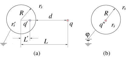
Figure 5: Images in a conducting sphere in the presence of monovalent salt with screening radius $r_{s}$: (a) a point charge $q$ induces an image charge $q^{\prime}=-Rq/L$ with a virtual cloud of monovalent ions with screening radius $r_{s}^{\prime}=Rr_{s}/L$; (b) a conducting sphere with potential $\phi$ is equivalent to a point charge $q^{\prime\prime}=DR\phi e^{R/r_{s}}$ with a virtual cloud of monovalent ions with screening radius $r_{s}$.

As a more complicated situation, let us consider a point charge $q$ and a grounded conducting sphere in a water solution with monovalent salt described by $r_{s}$ (Fig. 5a). As well known Landau , when $r_{s}\rightarrow\infty$, the magnitude and position of the image charge are given by (see Fig. 5 for definition of all lengthes)

$$q^{\prime}=-q\frac{R}{L},\ \ L^{\prime}=\frac{R^{2}}{L}.$$ (28)

When $r_{s}$ is finite, similar to the case of metallic semi-space, a virtual cloud of monovalent ions should be created together with the image charge. Due to the special geometry of a sphere, as one can check, the screening radius of this virtual cloud is given by

$$r_{s}^{\prime}=\frac{Rr_{s}}{L},$$ (29)

different from $r_{s}$ in the solution.

Another relevant situation is a conducting sphere with fixed potential $\phi$ in a water solution (see Fig. 5b). In this case, the potential in the solution can be solved exactly using linearized Poisson-Boltzmann equation and interpreted by the method of images. Actually it is equivalent to the potential produced by a image charge $q^{\prime\prime}$ at the center of the sphere. We can create a virtual cloud of monovalent salt together with the image charge as our convenience. The magnitude of $q^{\prime\prime}$ is then determined not only by the boundary condition but also the virtual cloud we choose. As we will see in the next subsection, it is convenient to introduce $r_{s}$ inside the sphere and get

$$q^{\prime\prime}=DR\phi e^{R/r_{s}}.$$ (30)

Let us calculate the interaction energy between a point charge and a grounded conducting sphere (Fig. 5a) for the purpose of the next subsection. Considering the interaction energy between $q$ and $q^{\prime}$, we have

$$U = \frac{qq^{\prime}}{2D(L-L^{\prime})}e^{-(R-L^{\prime})/r_{s}^{\prime}}e^{-(L-R)/r_{s}}$$ (31)

$$= -\frac{Rq^{2}}{2D(L^{2}-R^{2})}e^{-2d/r_{s}},$$

where $d=L-R$. In the limit of $r_{s}\rightarrow\infty$, the exponential factor goes to 1 and the energy goes back to the standard expression. The additional factor $e^{-2d/r_{s}}$ can be understood in the following way. The charge induced by $q$ on the surface of the sphere is proportional to $e^{-d/r_{s}}$, the interaction with it is also proportional to $e^{-d/r_{s}}$.

IV.2 Two spheres of the same size

Now we consider the interaction between two conducting spheres of the same size (see Fig. 3a) in the presence of monovalent salt. Due to the complexity of the method of images in the present case, instead of giving the general expression for the force, we focus on two limits: $d\gg r_{s}$ and $d\ll r_{s}$.

Let us first discuss the case when $d\gg r_{s}$. As well known, when $r_{s}\rightarrow\infty$, there is an infinite series of image charges in each sphere Smythe . For finite $r_{s}$, similar to what we discussed in the last subsection, the magnitudes and positions of all image charges are the same but a virtual cloud of monovalent salt is created together with each of them. In the particular case of $d\gg r_{s}$, we can actually cut off the infinite series and include the contribution from the leading order image charges only. To see this, one just remember that the image charges really represent surface charge densities induced on the two spheres. Each image in the infinite series gives a correction to the surface charge density calculated from the previous order image. As we discussed after Eq. (31), the new correction induced gets one more factor $e^{-d/r_{s}}$ . Since $d\gg r_{s}$, higher order corrections are exponentially small and can be completely neglected.

Figure 6: The first two image charges induced in each sphere in considering the interaction between two spheres. Each image charge has its own virtual cloud (not shown).

In Sec. III, the energy is calculated using capacitances (Eq. (12)). In the present case, it is more convenient to consider interaction energy between image charges directly. The two methods are equivalent providing that a factor $1/2$ is added to the interaction energy between a charge and its image Landau in the later method (see Eq. (LABEL:UL)). The two image charges in each sphere are given by (see Fig. 6)

$$q_{1} = DR\phi_{1}e^{R/r_{s}},\ \ q_{2}=DR\phi_{2}e^{R/r_{s}},$$ (32a)

$$q_{1}^{\prime} = -\frac{DR^{2}\phi_{2}}{L}e^{R/r_{s}},\ \ q_{2}^{\prime}=-\frac{DR^{2}\phi_{1}}{L}e^{R/r_{s}}.$$ (32b)

Here $q_{1}$ and $q_{2}$ are zero order image charges in each sphere which take into account of $\phi_{1}$ and $\phi_{2}$ respectively, similar to $q^{\prime\prime}$ discussed in the last subsection (see Eq. (30) and Fig. 5b). The screening radius accompanied with them is just $r_{s}$. The first order image charges $q_{1}^{\prime}$ and $q_{2}^{\prime}$ induced by $q_{2}$ and $q_{1}$ are accompanied by $r_{s}^{\prime}=Rr_{s}/L$, similar to $q^{\prime}$ discussed in the last subsection (see Eqs. (28), (29) and Fig. 5a). Similar to Eq. (31), the interaction energies between these images are

$$U(q_{1},q_{2}) = \frac{DR^{2}\phi_{1}\phi_{2}}{L}e^{-d/r_{s}},$$ (33)

$$U(q_{1},q_{2}^{\prime}) = -\frac{DR^{3}\phi_{1}^{2}}{L^{2}-R^{2}}e^{-2d/r_{s}},$$ (34)

$$U(q_{2},q_{1}^{\prime}) = -\frac{DR^{3}\phi_{2}^{2}}{L^{2}-R^{2}}e^{-2d/r_{s}},$$ (35)

and

$$U(L) = U(q_{1},q_{2})+\frac{1}{2}[U(q_{1},q_{2}^{\prime})+U(q_{2},q_{1}^{\prime})]$$

$$= \phi_{1}\phi_{2}\frac{DR^{2}}{L}e^{-d/r_{s}}-\frac{\phi_{1}^{2}+\phi_{2}^{2}}{2}\frac{DR^{3}}{L^{2}-R^{2}}e^{-2d/r_{s}}.$$

Correspondingly,

$$F(L) = \phi_{1}\phi_{2}\frac{DR^{2}}{L}e^{-d/r_{s}}\left(\frac{1}{r_{s}}+\frac{1}{L}\right)$$

$$- (\phi_{1}^{2}+\phi_{2}^{2})\frac{DR^{3}}{L^{2}-R^{2}}e^{-2d/r_{s}}\left(\frac{1}{r_{s}}+\frac{L}{L^{2}-R^{2}}\right).$$

We see clearly that an additional factor of $e^{-d/r_{s}}$ appears for each order of interaction. When $r_{s}\rightarrow\infty$, this equation goes back to Eq. (21) as expected.

At $d\gg r_{s}$, the first term in Eq. (LABEL:FLrs) dominates. When $\phi_{1}=\phi_{2}$, we have the standard double layer repulsion of DLVO theory Colloid . When $\phi_{1}$ and $\phi_{2}$ have same signs, only the second term represents attraction, which is negligible comparing with repulsion. This is analogous to Eq. (21) but attraction is much weaker here. So in the limit of $d\gg r_{s}$, the force is attractive only if potentials are opposite in signs or one of potentials is equal to zero.

Now let us consider the case when $d\ll r_{s}$. In this case, the factor $e^{-d/r_{s}}\simeq 1$ and all higher order image charges should be included. Since each image charge is accompanied by its own virtual cloud, the interaction is very complicated. Instead of calculating it exactly, we estimate $C_{11}$ and $C_{12}$ using a simple method as follows. We divide the surface of the two spheres into two pieces. In the first piece, the distance between the surfaces of the two spheres is smaller than $r_{s}$ so that the two spheres interact with each other in an unscreened Coulomb way. We call this piece “contact region” (see Fig. 7). In the second piece, the distance between the two surfaces is larger than $r_{s}$ and the interaction between them is exponentially small and negligible. Therefore, we can safely assume that the modification to the capacitances of the two spheres due to their proximity happens only in the contact region.

Figure 7: A schematic illustration of the contact region between two spheres. The contact region includes the surfaces of two spheres inside a cylinder with the cross section shown by the rectangular.

In order to calculate $C_{11}$ and $C_{12}$, let us first consider a special case when $\phi_{1}=\phi_{2}=\phi$. In this case, the charge induced on two spheres are equal and given by $\phi(C_{11}+C_{12})$. In the contact region, the screening effect by monovalent salt can be ignored and the adjacent spots of the two spheres form a capacitor with zero voltage, therefore the charge is zero Rui . While for the rest part of the sphere, the interaction between two spheres is exponentially small and the charge on each sphere is almost the same as if the other sphere is not there. Therefore we have

$$C_{11}+C_{12}=\frac{DR^{2}}{r_{s}}-\frac{DR(r_{s}-d)}{4r_{s}}.$$ (38)

Here $DR^{2}/r_{s}$ is the capacitance of a single sphere in the presence of monovalent salt. When the sphere gets close to the other sphere, it loses its capacitance in the contact region, whose area is $\pi R(r_{s}-d)$.

Then we consider another special case when $\phi_{1}=-\phi_{2}=\phi$. In this case, we have $q_{1}=(C_{11}-C_{12})\phi=-q_{2}$. Outside the contact region, the capacitance is the same as in the previous case. Inside the contact region, the capacitance can be estimated as

$$C=D\int^{\theta_{0}}_{0}\frac{dS}{x(\theta)}=D\int^{\theta_{0}}_{0}\frac{2\pi R^{2}sin\theta d\theta}{d+2R(1-cos\theta)}=\pi DR\ln\frac{r_{s}}{d},$$ (39)

where $\theta_{0}$ is the angle for the boundary of the contact region (see Fig. 7). The absolute value of the charge induced on each sphere in the contact region is $2C\phi$. Therefore

$$C_{11}-C_{12}=\frac{DR^{2}}{r_{s}}-\frac{DR(r_{s}-d)}{4r_{s}}+2\pi DR\ln\frac{r_{s}}{d}.$$ (40)

Combining Eqs. (38) and (40), we get

$$C_{11} = \frac{DR^{2}}{r_{s}}-\frac{DR(r_{s}-d)}{4r_{s}}+\pi DR\ln\frac{r_{s}}{d},$$ (41a)

$$C_{12} = -\pi DR\ln\frac{r_{s}}{d}.$$ (41b)

In the case of $r_{s}\sim R$, these results match Eq. (22) which was obtained for $r_{s}\gg R$.

Using Eq. (14), and remembering $d\ll r_{s}$, we have

$$F=-\frac{\pi DR}{2d}(\phi_{1}-\phi_{2})^{2}.$$ (42)

The force is independent of $r_{s}$ in this limit because the change of capacitances happens mainly in the contact region (the logarithm term in Eq. (41)). Again, the attraction shows up at small $d$ and the attractive force decays as a power law. For the model of conductors to work, we require $d\gg A$ which is valid since $A\ll r_{s}$.

IV.3 A small sphere and a big sphere

Now we consider the interaction between a small sphere and a big sphere (see Fig. 3b) in the presence of monovalent salt. The approach we used is similar to that in the last subsection.

When $d\gg r_{s}$, calculating the interaction between leading order image charges similar to Eq. (LABEL:FLrs), we get

$$F(L) = \phi_{1}\phi_{2}\frac{DR_{1}R_{2}}{Lr_{s}}e^{-d/r_{s}}$$ (43)

$$- \left(\frac{R_{1}\phi_{1}^{2}}{L^{2}-R_{2}^{2}}+\frac{R_{2}\phi_{2}^{2}}{L^{2}-R_{1}^{2}}\right)\frac{DR_{1}R_{2}}{r_{s}}e^{-2d/r_{s}}.$$

Again, when $\phi_{1}$ and $\phi_{2}$ have the same signs, attraction is exponentially weaker in this limit. When $d\ll r_{s}$, we can estimate $C_{11}$, $C_{12}$ and $C_{22}$ similar to Eq. (41). We get an attractive force given by Eq. (1).


In the end of this section, let us discuss the possibility of nonlinear screening by monovalent salt in a special case when $\phi_{1,2}>0$. The result can be generalized to other cases. The condition for linear screening reads

$$\phi_{1,2}<\phi_{c}=\frac{k_{B}T}{e}|\ln(cv_{0})|,$$ (44)

where $e$ is the proton charge and $c$ and $v_{0}$ are the concentration and volume of the monovalent ion. Here $\phi_{c}$ is determined by entropy of monovalent ions in the solution. According to Eqs. (4) and (11), $\phi_{1,2}\lesssim Ze/Dr_{1,2}\ll Ze/Da$, where $a\ll r_{1,2}$ is the radius of a $Z$-ion (see Fig. 2). If $\phi_{1,2}>\phi_{c}$, $Ze/Da\gg\phi_{c}$. Therefore monovalent counterions are adsorbed to $Z$-ions. As a result, the effective charge of a $Z$-ion is renormalized to

$$Z^{\ast}e=Da\phi_{c}.$$ (45)

This effective charge is not changed when a $Z$-ion is adsorbed on the surface of the macroion since $Z^{\ast}e/Dr_{1,2}\ll Z^{\ast}e/Da$. Consequently, $\phi_{1,2}$ should be calculated using $Z^{\ast}$ and satisfy $\phi_{1,2}<Z^{\ast}e/Da=\phi_{c}$. In summary, the nonlinear screening of monovalent salt is important when $Z$-ions are strongly charged. In this case, our theory is still applicable providing that $Z$ is replaced by $Z^{\ast}$ everywhere.

V attraction of two macroions, when only one of them adsorbs $Z$-ions

In this section, we generalize our theory to a little more complicated case when the two bare macroions are oppositely charged. As shown in Fig. 1a, Positive $Z$-ions are only adsorbed to the negative probe and invert its charge. In the presence of large concentration of monovalent salt, monovalent counterions are adsorbed to the positive surface (nonlinear screening), reducing its electric potential to $\phi_{c}$ (see Eq. (44)). This potential is certainly different from the electric potential of the probe determined by $Z$-ions (Eq. (11)). We again have two conductors with different fixed potentials. Even when both potentials are positive (the net charges of the surface and the probe are positive), the force is still attractive at small distances as we discussed in the last section.

The atomic force experiment in Ref. Lemay is actually a realization of the situation discussed above. The maximum of the repulsive force mentioned in introduction can be understood following Eq. (43), extrapolated to $d\simeq r_{s}$. When both potentials are positive, at $d\gg r_{s}$, the first term (repulsion term) in Eq. (43) dominates and the force is repulsive. At $d\lesssim r_{s}$ ($r_{s}\simeq 100$ $\AA$ in the experiment), the second, attraction term in Eq. (43) dominates due to its larger pre-factor of the exponential. This leads to the maximum of the repulsion at $d\simeq r_{s}$. When $d\ll r_{s}$, we have the polarization attraction given by Eq. (1).

For $d<r_{s}$, Eq. (3) can be used to compare the polarization attraction with the van der Waals one. According to discussions in introduction and Sec. II, we conclude that for substantial difference between $\sigma_{1}$ and $\sigma_{2}$, the polarization force $F_{p}$ is much larger than $F_{vdW}$ at $d\gg A$ ($A=21$ $\AA$ for $Z=3$ and $-\sigma=-0.75$ e/nm²). Therefore the van der Waals attraction has nothing to do with the attraction observed in the experiment at $d\simeq 100$ $\AA$.

So far we have considered two cases when the electric potentials of the two macroions are different and the attraction between likely charged macroions is possible. One is that positive $Z$-ions are adsorbed to both negative macroions; the other is that positive $Z$-ions are only adsorbed to one negative macroion, but monovalent counterions are adsorbed (nonlinearly screening) to the other positive macroion. It is interesting to relate them to the more standard case when two likely charged (say, negative) macroions are nonlinearly screened by positive monovalent counterions (no $Z$-ions in the solution). In this case, the two macroions have the same electric potential $\phi_{c}$ given by Eq. (44) and never attract each other Colloid .

VI Conclusion

In this paper, we discussed a long range polarization attraction of two likely charged spherical macroions in the presence of multivalent counterions ($Z$-ions). We show that the necessary condition for the attraction is that the bare charge densities of the two macroions are different. This polarization attraction is much stronger and longer ranged than the van der Waals force Colloid and the short range correlation attraction Bloomfield . In the presence of large amount monovalent salt, it adds an additional term to the standard double layer repulsion of DLVO theory when the two macroions are different. We discussed two cases when the polarization force between two different macroions can be attractive, even if their net charges have the same sign. In the first case, both macroions adsorb $Z$-ions (Fig. 1b). In the second case, one macroion adsorbs $Z$-ions while the other adsorbs monovalent counterions (Fig. 1a). Here “adsorb” means that the binding energy is much larger than $k_{B}T$. In both cases, due to different equilibrium conditions of adsorbed ions, the electric potentials of two macroions are different and the attraction is possible. On the other hand, the attraction is impossible if two macroions are likely charged and both adsorb monovalent counterions (no $Z$-ions in the solution). Our result qualitatively agrees with atomic force experiments Lemay ; Sivan .

Even though in this paper we only discuss spherical macroions, the polarization attraction we discovered can be generalized to other geometries. Actually, as seen before, the attraction is always developed at small distances between macroions when the overall geometry is not very important. One can also understand this using the language of contact electrification as discussed in the introduction.

In this paper, in the connection with atomic force experiments Lemay ; Sivan , we focused on the force between two macroions instead of the total free energy of the system. Actually, for typical situations (e.g., $A\ll R$ or $A\ll r_{s}$), one can show that the free energy may have the global minimum when the two macroions are close to each other. Thus, the polarization attraction can play an important role in determining the equilibrium state of the system. It answers the gene delivery related question: even if charges of DNA and cell membrane are both inverted, they can still be attracted to each other since DNA and membrane certainly have different surface charge densities. It can also be important for aggregation or self-assembly of large ensembles of different likely charged macroions with help of oppositely charged $Z$-ions. Assume for example that we have a mixture of equal numbers of two kinds of negative spheres with the same radius but different values of the bare charges. Then in the presence of positive $Z$-ions, they can attract each other and assemble in a NaCl-like structure. *

Appendix A

Let us start from the asymptotic behavior of the series $\sum_{n=1}^{\infty}1/\sinh nt$ at $t\rightarrow 0$. According to the Cauchy Integral test of convergence, we have

$$\int_{1}^{\infty}\frac{1}{\sinh xt}dx\leq\sum_{n=1}^{\infty}\frac{1}{\sinh nt}\leq\int_{1}^{\infty}\frac{1}{\sinh xt}dx+\frac{1}{\sinh t}.$$ (46)

Evaluating the integral, we have

$$\frac{1}{2t}\ln\frac{\cosh t+1}{\cosh t-1}\leq\sum_{n=1}^{\infty}\frac{1}{\sinh nt}\leq\frac{1}{2t}\ln\frac{\cosh t+1}{\cosh t-1}+\frac{1}{\sinh t}.$$ (47)

In the limit of $t\rightarrow 0$, it becomes

$$\frac{1}{t}\ln\frac{2}{t}<\sum_{n=1}^{\infty}\frac{1}{\sinh nt}<\frac{1}{t}\ln\frac{2e}{t}.$$ (48)

Therefore in this limit, we have

$$\sum_{n=1}^{\infty}\frac{1}{\sinh nt}=\frac{1}{t}\ln\frac{2\beta}{t},$$ (49)

where $\beta$ is a number satisfying $1<\beta<e$. Replacing $t$ by $2t$, we get

$$\sum_{n=1}^{\infty}\frac{1}{\sinh 2nt}=\frac{1}{2t}\ln\frac{\beta}{t}.$$ (50)

And

$$\sum_{n=1}^{\infty}\frac{1}{\sinh(2n-1)t}=\sum_{n=1}^{\infty}\frac{1}{\sinh nt}-\sum_{n=1}^{\infty}\frac{1}{\sinh 2nt}=\frac{1}{2t}\ln\frac{4\beta}{t}.$$ (51)

Since $\cosh t=(2R+d)/2R$, the limit of $t\rightarrow 0$ is equivalent to $d\rightarrow 0$ and $t=\sqrt{d/R}$ in this limit. According to Eq. (15), we have

$$C_{11} = \frac{DR}{4}\ln\frac{16\beta^{2}R}{d},$$ (52a)

$$C_{12} = -\frac{DR}{4}\ln\frac{\beta^{2}R}{d}.$$ (52b)

Numerical calculation gives $\beta=1.78$.

- (1) A. Yu. Grosberg, T. T. Nguyen, and B. I. Shklovskii, Rev. Mod. Phys. 74, 329 (2002).
- (2) K. Besteman, M. A. G. Zevenbergen, H. A. Heering, and S. G. Lemay, Phys. Rev. Lett. 93, 170802 (2004).
- (3) B. I. Shklovskii, Phys. Rev. E 60, 5802 (1999).
- (4) U. Sivan, private communication.
- (5) B. V. Derjaguin and L. D. Landau, Acta Physicochimica (URSS) 14, 633 (1941). E. J. W. Verwey and J. Th. G. Overbeek, Theory of the stability of lyophobic colloids (Elsevier, Amsterdam, 1948). D. F. Evans and H. Wennerström, The colloidal domain, 2nd ed. (Wiley-VCH, New York, 1999).
- (6) I. Rouzina and V. A. Bloomfield, J. Phys. Chem. 100, 9977 (1996). A. G. Moreira and R. R. Netz, Phys. Rev. Lett. 87, 078301 (2001).
- (7) L. D. Landau, E. M. Lifshitz, and L. P. Pitaevskii, Electrodynamics of continuous media, 2nd ed. (Butterworth-Heinemann, Oxford, 1995).
- (8) R. Messina, C. Holm, and K. Kremer, Europhys. Lett. 51, 461 (2000).
- (9) W. R. Smythe, Static and dynamic electricity, 3rd ed. (Hemisphere, NewYork, 1989).
- (10) In this case, one can show that the polarization attraction still exist, although its theory is more complicated.
- (11) R. Zhang and B. I. Shklovskii, Phys. Rev. E 69, 021909 (2004).