Stability of the shell structure in 2D quantum dots

Abstract

We study the effects of external impurities on the shell structure in semiconductor quantum dots by using a fast response-function method for solving the Kohn-Sham equations. We perform statistics of the addition energies up to 20 interacting electrons. The results show that the shell structure is generally preserved even if effects of high disorder are clear. The Coulomb interaction and the variation in ground-state spins have a strong effect on the addition-energy distributions, which in the noninteracting single-electron picture correspond to level statistics showing mixtures of Poisson and Wigner forms.

I Introduction

The functionality of nanoelectronic devices strongly depends on the quality of the samples produced in the fabrication process. In semiconductor quantum dots (QD), qd there may exist external impurities, which have considerable effects on the measurable quantities such as the addition energy and the chemical potential. Generally, the physical properties of QD’s can be determined by the shape of the confining potential restricting the electrons in the semiconducting material.

In a vertical QD formed in a double-barrier heterostructure, the measured addition energies (cf. electron affinities) correspond well to the shell structure of a two-dimensional parabolic (harmonic) model potential. tarucha Remarkably good agreement between the experiment and theory has been obtained by using this model and taking the electron-electron interactions into account by employing, e.g., the spin-density-functional theory (SDFT). hirose2 ; reimann There are, however, always sample-specific variations matagne such that in QD’s with more than only a few electrons, the agreement between the experiments and theory becomes generally worse, presumably due to non-symmetric deviations of the actual confining potential.

Deviations from the circular symmetry can be induced by impurity particles migrated through the heterostructure layers. States bound to hydrogenic impurities were found in the single-electron tunneling experiment by Ashoori et al. ashoori Recently, a clear deformation in the transport spectrum of a resonant tunneling device was shown to be due to an ionized single or double-acceptor near the QD. esa6 For the time being, there is no experimental data showing systematic impurity effects, but the eventual serial production of QD structures can lead to a considerable fraction of distorted samples.

Theoretical research of QD’s containing impurities has been mostly based on either single-impurity systems studied with exact diagonalization halonen and the SDFT, esa6 or on QD’s with a relatively high impurity density. hirose1 ; gycly In the latter case, Hirose et al. hirose1 have performed SDFT studies on the energy fluctuations and the effects of interactions, as well as on the role of spin. hirose3 These systems have experimental realization in disordered (no shell structure) QD’s, where the fluctuations in the Coulomb blockade peak spacings show interesting statistics beyond the constant interaction model combined with the random matrix theory. sivan ; berkovits

In this paper we focus on the stability of the shell structure in primarily parabolic few-electron QD’s. Particularly, the effects of external impurities on the addition energies are studied up to the high-disorder limit. The two main extensions to previous studies are (i) the use of an impurity model based on recent experimental findings esa6 and (ii) the computation of the complete addition energy spectrum up to 20 electrons with both a single impurity at an arbitrary position, and finally with an ensemble of one thousand impurity configurations. The calculations are performed using the SDFT with a remarkably fast response-function iteration method for the Kohn-Sham (KS) equations. michael The resulting spectra demonstrate that the shell structure is generally preserved, although in the mid-shell regime there can be drastic changes in the energetics. The statistics of the noninteracting level spacings can be characterized by a mixture of Poisson and Wigner distributions. Those shapes are strongly affected by the Coulomb interaction and by the ground-state spins.

The organization of this paper is as follows. First in Sec. II we define the model system and the parameters for the external impurities. In Sec. III we introduce the response-function scheme for the density-functional calculations. The results for a single repulsive impurity are presented in Sec. IV. Finally the addition-energy distributions from one thousand configurations are shown in Sec. V. The paper is summarized in Sec. VI.

II Model

We model the quantum dot by using the conventional effective-mass approximation and choose the material parameters for GaAs, i.e., the effective mass $m^{*}=0.067\,m_{e}$ and the dielectric constant $\epsilon=12.7$. We apply a strictly two-dimensional model by assuming a negligible degree of freedom for electrons in the vertical direction. The many-electron Hamiltonian is given in the effective atomic units units as

$$H=\sum^{N}_{i=1}\left[-\frac{\nabla^{2}_{i}}{2}+\frac{1}{2}\omega_{0}^{2}r_{i}^{2}+V_{\rm imp}({\mathbf{r}}_{i})\right]+\sum^{N}_{i<j}\frac{1}{|{\mathbf{r}}_{i}-{\mathbf{r}}_{j}|},$$ (1)

where $\omega_{0}$ defines the strength of the external confinement, which is assumed to be parabolic in shape. The Coulomb potential caused by the $N_{\rm imp}$ impurity particles located in the vicinity of the QD and having charges $|q_{k}|$, is written as

$$V_{\rm imp}({\mathbf{r}})=\sum^{N_{\rm imp}}_{k=1}\frac{|q_{k}|}{\sqrt{({\mathbf{r}}-{\mathbf{R}}_{k})+d_{k}}},$$ (2)

where ${\mathbf{R}}_{k}$, and $d_{k}$ define the lateral and vertical positions of the particles. This model has been shown to result in a good agreement with the measured transport spectrum of a vertical QD. esa6

In the first calculations, we include a single impurity with a negative unit charge on the QD plane ($d=0$) and vary only the lateral position $R$. Further, when performing a statistical analysis, we assume that there exist $1-10$ randomly distributed impurity particles migrated in the tunneling barrier of the QD. We choose the ranges for the impurity positions as $0\leq R_{k}\leq 10\,a^{*}_{B}$ and $0\leq d_{k}\leq 1\,a^{*}_{B}$. We set $q_{k}=-1$ which is in a qualitative accordance with the results from the tunneling experiments. esa6 In addition, the minimum spacing between two impurities is expected to be $0.1\,a^{*}_{B}$ which is of the order of the lattice constant for the layer material (e.g., AlGaAs).

III Method

The numerical procedure for solving the electronic properties of the system defined above is based on the spin-density-functional theory (SDFT). In the self-consistent Kohn-Sham formulation, the effective Schrödinger equation to be solved iteratively is written as

$$\left[-\frac{\nabla^{2}}{2}+V_{\rm KS}({\mathbf{r}})\right]\Phi_{i}^{\sigma}(\mathbf{r})=\epsilon_{i}\Phi_{i}^{\sigma}(\mathbf{r}),$$ (3)

where the Kohn-Sham potential $V_{\rm KS}$ is a sum of the external potential defined above, the Hartree potential, and the exchange-correlation potential given as $V_{\rm xc}({\mathbf{r}})=\delta{E_{xc}}[\rho,\xi]/\delta\rho^{\sigma}{({\mathbf{r}})}$. Here $\rho$ is the electron density, $\sigma$ denotes the spin index, and $\xi(\mathbf{r})=[\rho^{\uparrow}(\mathbf{r})-\rho^{\downarrow}(\mathbf{r})]/\rho(\mathbf{r})$ is the spin polarization. For $E_{xc}$ we use the local spin-density approximation based on the functional provided by Attaccalite and co-workers. attaccalite

A detailed description of the following algorithms can be found in Refs. newton, ; collective, ; michael, . We start with solving for the lowest $n$ solutions of the eigenvalue problem (3) by applying the evolution operator,

$$\mathcal{T}(\epsilon)\equiv\text{e}^{-\epsilon H}$$ (4)

repeatedly to a set of states $\{\psi_{j},\,1\leq j\leq n\}$, and orthogonalizing the states after every step. Instead of the commonly used second-order factorization in combination with the Gram-Schmidt orthogonalization, we use the fourth-order factorization for the evolution operator imstep given by

$$\mathcal{T}^{(4)}\equiv\text{e}^{-\frac{1}{6}\epsilon V}\text{e}^{-\frac{1}{2}\epsilon T}\text{e}^{-\frac{2}{3}\epsilon\tilde{V}}\text{e}^{-\frac{1}{2}\epsilon T}\text{e}^{-\frac{1}{6}\epsilon V}=\text{e}^{-\epsilon[H+\mathcal{O}(\epsilon^{4})]}.$$ (5)

For the orthonormalization, we diagonalize the matrix of overlap integrals and construct from these a new set of orthonormal states. Depending on the physical system this method can be faster by up to a factor of 100 in comparison to the second-order factorization.

A widespread problem of the density-functional calculations is the large number of iterations required to obtain a self-consistent solution. Namely, to maintain the stability of the iteration process, it is necessary to keep the mixing parameter(s) small, which can lead to thousands of iterations. We overcome this problem with a procedure having its roots in the Hohenberg-Kohn theorem which states that the one-body density $\rho(\mathbf{r})$ is the only truly independent variable. Therefore an algorithm which solves for $\rho(\mathbf{r})$ directly by applying a Newton-Raphson procedure is used. We define

$$\Delta\rho^{\sigma}(\mathbf{r})=\sum_{\mathbf{h}}n^{\sigma}(\mathbf{h})|\Phi^{\sigma}_{\mathbf{h}}[\rho^{\uparrow},\rho^{\downarrow}](\mathbf{r})|^{2}-\rho^{\sigma}(\mathbf{r})$$ (6)

as the density difference between two self-consistent iterations. Here $n^{\sigma}$ is the occupation factor, $\Phi^{\sigma}_{\mathbf{h}}$ are the orthogonalized solutions of Eq. (3), and $\rho^{\sigma}(\mathbf{r})$ is the density used for the calculation of $V_{\rm KS}$. The sum is over all occupied (hole: $\mathbf{h}$) states. Then the density correction $\delta\rho^{\sigma}(\mathbf{r})$ is determined by a linear equation

$$\Delta\rho^{\sigma}(\mathbf{r})=\sum_{\sigma^{\prime}}\int d^{d}r^{\prime}\,\varepsilon^{\sigma,\sigma^{\prime}}(\mathbf{r},\mathbf{r^{\prime}};0)\delta\rho^{\sigma^{\prime}}(\mathbf{r}^{\prime}).$$ (7)

Here $d$ is the dimension of the system and $\varepsilon^{\sigma,\sigma^{\prime}}$ is the static dielectric function of a non-uniform electron gas. PinesNoz It contains the zero-frequency Lindhard function and $V_{p-h}^{\sigma,\sigma^{\prime}}(\mathbf{r},\mathbf{r^{\prime}})=\delta V_{\rm KS}^{\sigma}(\mathbf{r})/\delta\rho^{\sigma^{\prime}}(\mathbf{r^{\prime}})$. To avoid the calculation of unoccupied (particle: $\mathbf{p}$) states we seek for an approximation for the static response function that only needs the calculation of occupied states. For that purpose, we recall that linear response theory can be derived ThoulessBook from an action principle for excitations of the form $\left|\psi(t)\right\rangle=\exp(\sum_{ph}c_{ph}(t)a^{\dagger}_{p}a_{h})\left|\phi_{0}\right\rangle$, where $\left|\phi_{0}\right\rangle$ is the ground state, and $c_{ph}(t)$ are particle–hole amplitudes. If we assume that the particle–hole amplitudes are matrix elements of a local one-body operator $c^{\sigma}({\bf r})$, we end up with Feynman’s theory of collective excitations. Feynman In this approximation, we can rewrite Eq. (7) as

$$\left[-\frac{1}{2}\nabla\cdot\left[\rho^{\sigma}(\mathbf{r})\nabla\right]+2\sum_{\sigma^{\prime}}S_{F}^{\sigma}\,\star\,V^{\sigma,\sigma^{\prime}}_{p-h}\,\star\,S_{F}^{\sigma^{\prime}}\,\star\right]w^{\sigma^{\prime}}$$

$$=2\sum_{\sigma^{\prime}}S_{F}^{\sigma}\,\star\,V^{\sigma,\sigma^{\prime}}_{p-h}\,\star\,\Delta\rho^{\sigma^{\prime}},$$ (8)

where now

$$\delta\rho^{\sigma}(\mathbf{r})\,=\,\Delta\rho^{\sigma}(\mathbf{r})-S^{\sigma}_{F}(\mathbf{r},\mathbf{r^{\prime}})\,\star\,{w}^{\sigma}(\mathbf{r^{\prime}}),$$ (9)

and

$$S_{F}^{\sigma}(\mathbf{r},\mathbf{r}^{\prime})=\rho^{\sigma}(\mathbf{r})\delta(\mathbf{r}-\mathbf{r^{\prime}})-\frac{1}{2}\left|\sum_{\mathbf{h}}\Phi^{\sigma}_{\mathbf{h}}(\mathbf{r})\Phi^{\sigma}_{\mathbf{h}}(\mathbf{r^{\prime}})\right|^{2},$$ (10)

which is proportional to the static structure function of the noninteracting system. Above, the asterisk stands for the convolution integral. With these manipulations, we have rewritten the response-iteration equation in a form that requires only the calculation of the occupied states. Since the multiplication of the left-hand side of Eq. (8) requires only vector–vector operations, the equation can be solved with the conjugate–gradient method.

IV Single impurity

Figure 1 shows the addition energies up to 20 electrons

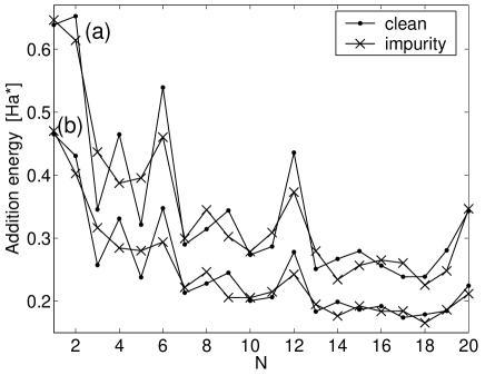
Figure 1: Addition energies for clean and impurity-containing QD’s with the confinement strengths of $\omega_{0}=5$ meV (a) and $3$ meV (b).

for two QD’s with $\omega_{0}=5$ and 3 meV. A single impurity particle with $q=-1$ is located on the QD plane ($d=0$) at $R=2\,l_{0}$, where $l_{0}=\sqrt{1/m^{*}\omega_{0}}$, giving $R=3.00\,a^{*}_{B}$ and $3.87\,a^{*}_{B}$ for $\omega_{0}=5$ and 3 meV, respectively. The addition energies of the corresponding clean (no impurity) QD’s are also presented. They qualitatively agree with the previous SDFT results by Reimann et al. reimann and Hirose and Wingreen hirose2 for $\omega_{0}\sim 3$ meV [Fig. 1(b)]. Increasing the confinement strength to $5$ meV leads to the disappearance of the even peaks at $N=14\ldots 18$, but the ground-state spins remain the same, having the well-known sequence determined by Hund’s rule. hirose2

In the presence of the impurity, the peaks at magic electron numbers ($N=2,6,12,20$) are preserved. In contrast, the peaks at $N=4$ and $9$ which in the clean case correspond to aligned spins in the 2nd and 3rd shells, are strongly diminished and the ground-state spins are $S=0$ and $1/2$, respectively. Generally, the inclusion of a single impurity worsens the agreement between the calculated addition-energy spectrum and the experimental result by Tarucha and co-workers. tarucha

Next we study how the energetics depends on the location of the impurity particle on the QD plane. The results presented below have been calculated using the fixed confinement strength of $\omega_{0}=5$ meV. Figure 2 shows the

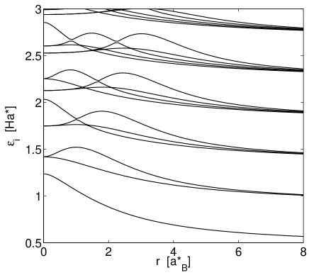
Figure 2: Noninteracting single-electron energies for a quantum dot containing a single repulsive impurity particle on the dot plane ($d=0$) and at $R=0\ldots 8\,a^{*}_{B}$ from the center.

noninteracting single-electron energies as a function of $R$. At large $R$, the energies approach the shells of a clean QD with $\epsilon_{nl}=(2n+|l|+1)\omega_{0}$, whereas $R=0$ corresponds to the eigenenergies of a finite-width quantum ring chakraborty with several doubly-degenerated shells. The mid-$R$ range is characterized by many avoided crossings between the states that a degenerate in the absence of the impurity.

We performed the SDFT calculations for $N=2\ldots 21$ and $R=0\ldots 7.5\,a^{*}_{B}$ with a step size of $0.1\,a^{*}_{B}$. For each $N$ and $R$, we calculated several states to find the correct ground-state energy and spin. The plot of the addition energies is shown in Fig. 3.

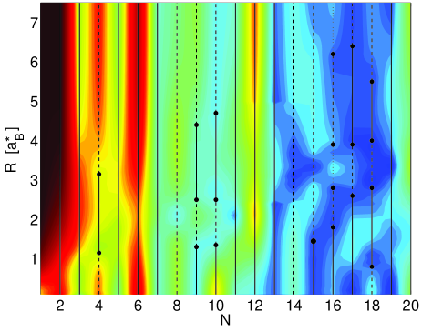
Figure 3: (color online) Addition energies (scale from dark blue to dark red) for a quantum dot containing a single repulsive impurity particle at $R=0\ldots 7.5\,a^{*}_{B}$ from the dot center. The filled circles denote the changes in the ground-state spin. The solid, dashed, and dotted lines correspond to $S=0$ or $1/2$, $S=1$ or $3/2$, and $S=2$ or $5/2$, respectively.

The values indicated by different colors in the figure vary between $0.22\,{\rm Ha}^{*}$ (dark blue) and $0.65\,{\rm Ha}^{*}$ (dark red). The dots with magic electron numbers remain particularly stable and paramagnetic ($S=0$) despite the impurity particle located at different radius from the center. The most apparent exception is $N=12$ at small $R$, showing a shift to $N=10$ as a stable configuration. This corresponds to a state with filled shells and $S=0$ in the quantum-ring-like geometry, as seen in Fig. 2. QD’s with $N=4,8,14,$ and $18$ have partially occupied highest shells in the both limits, leading to $S=1$ due to Hund’s rule. The constant $S=1$ ground state of $N=8$ and $14$ can be understood from the small energy gap between the 4th and 5th, as well as between the 7th and 8th eigenstates throughout the $R$ regime (Fig. 2).

In Fig. 4 we show examples of the electron densities for a 12-electron QD

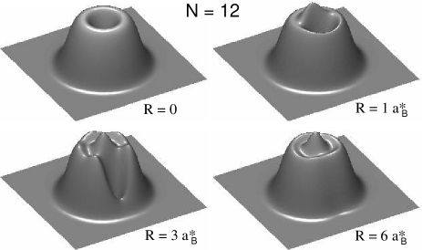
Figure 4: Electron densities of a 12-electron quantum dot with an impurity particle located at $R=0$, $1$, $3$, and $6\,a^{*}_{B}$ from the dot center, respectively.

with different impurity locations. The insertion of the impurity particle at the center ($R=0$) leads to a typical quantum-ring-like solution with the density distribution on the edge of the QD. As the impurity is located off the center, the density deforms gradually through a slightly localized shape with six peaks to a clean configuration where the circular symmetry is retained.

We also find many solutions, always corresponding to half-filled shells, where the spin symmetry is broken. These so-called spin-density waves (SDW) koskinen have been criticized by Hirose and Wingreen hirose2 , arguing that the solutions are mixtures of different (total) spin states, and thus artifacts of the SDFT. Recently, the claim was shown true explicitly in a rectangular four-electron QD by employing the SDFT and the exact diagonalization. ari Nevertheless, the total energy of the SDW solution is only slightly smaller than the exact energy and in any case it represents an improvement over the corresponding single-configurational DFT (spin-compensated) energy. Hence, the SDW solutions are included as such in the energetics considered in this paper.

V Random impurities

Then we include a random number (1-10) of negatively charged impurities randomly in the expected tunneling barrier below the QD (see Sec. II for the parameters). We computed 1000 impurity configurations such that for each configuration the number of electrons in the QD was $N=1\ldots 21$. To determine the groud-state spins in the many-electron problem, we calculated all the relevant ($S\leq 2$) spin states for each $N$.

V.1 Single-electron picture

We begin with the level statistics of a QD with noninteracting electrons. Now the electrons are affected only by the confining and impurity potentials. This corresponds to the single-electron picture where the addition energy is simply equal to the level spacing, $\Delta_{0}(N)=\epsilon_{N/2+1}-\epsilon_{N/2}$, where the divisor of two follows from the spin degeneracy. Fig. 5

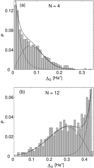
Figure 5: Noninteracting addition-energy distributions of 1000 impurity configurations corresponding to $N=4$ (a) and $N=12$ (b). The approximative contributions of the Poisson and Wigner-type distributions are also shown. The energy binwidth is $0.01\,{\rm Ha}^{*}$.

shows examples of the (noninteracting) addition-energy distributions as $N=4$ and 12. As the average impurity density is relatively low, there are several configurations that are close to the clean case, leading to a Poisson-like level distribution. On the other hand, the strongly distorted configurations lead to Wigner distribution. Thus, the sum of these subgroups give the observed double-peak shape which is pronounced in the 12-electron case [Fig. 5(b)]. The active region of the QD is then larger than that for $N=4$, leading to a higher number of distorted configurations since the impurity density is kept constant. In both cases, we have divided the configurations into these two parts in such a way that QD’s with a total energy higher than a certain, qualitatively chosen critical value are considered as “distorted” and the remaining configurations as “clean”. The fits corresponding to the sums of the Poisson and Wigner functions and $\Delta_{0}$ is plotted in Fig. 5. The distributions are mirror images of each other, since in the clean QD $N=12$ is a filled-shell case with $\Delta_{0}(12)\sim 0.45\,{\rm Ha}^{*}$, whereas $\Delta_{0}(4)=0$.

For QD’s, the level-spacing distributions are typically plotted by keeping the QD parameters as the external confinement or the magnetic field constant and considering high number of eigenstates within a certain energy range. The integrability of the system can then be connected to the level spacings such that the Wigner distribution is interpreted as a signature of quantum chaos. kaaos Our case is qualitatively similar in the sense that the varied parameter is the impurity configuration instead of the energy, and high distortion leads to the Wigner distribution as shown by Hirose and co-workers. hirose1 We suggest, however, that in isolated few-electron QD’s the average impurity density is considerably smaller than in their model, leading to a significant contribution of the Poisson-type level-spacing distribution as visualized in Fig. 5. We note here that Hirose et al. hirose1 defined the noninteracting picture such that the electrons do not interact with the impurities, while we consider the eigenenergies of a single electron in the presence of the impurity potential.

V.2 Interacting electrons

We examine the corresponding many-electron problem using the same 1000 randomly determined impurity configurations. Taking the different possibilities for each ground-state spin into account, we performed $\sim 70000$ self-consistent SDFT calculations. Figure 6

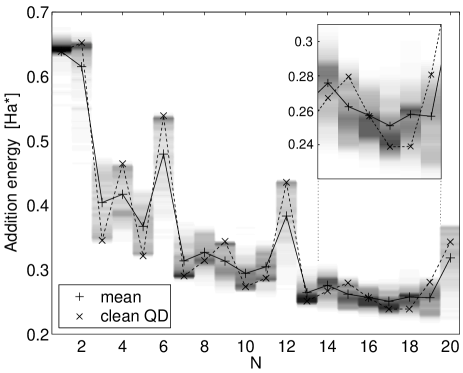
Figure 6: Addition-energy distributions of 1000 different impurity configurations in a quantum dot of 1-20 electrons. All the possibilities for the ground-state spins are taken into account.

shows the addition energy spectrum, where the distribution for each $N$ is plotted in grayscale. The mean values of the distributions are shown as pluses, and the crosses correspond to the clean, parabolic QD [repeated from Fig. 1(a)]. Particularly with small $N$, the result of the clean case matches rather accurately with the maxima of the distributions due to the relatively high fraction of non-distorted configurations. In the regime $13\leq N\leq 19$, there are clear deviations between the clean QD and the maxima, as visualized in the inset of Fig. 6 in more detail. The reason is the high degeneracy of different states in this regime and the increased tendency to distortion due to the relatively large active-dot region.

In Fig. 7

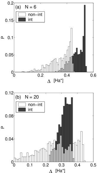
Figure 7: Addition-energy distributions for $N=6$ (a) and $N=20$ (b) quantum dots in noninteracting (white) and interacting (dark gray) cases.

we have a detailed look on the addition-energy distributions of $N=6$ and $20$ QD’s in comparison with the corresponding values for noninteracting QD’s defined in Sec. V.1. We have chosen these magic electron numbers to exclude the spin effects. Namely, in determining $\Delta(6)$ and $\Delta(20)$, practically all impurity configurations give $S=0$ and $1/2$ for these $N$ and $N\pm 1$, respectively. As expected, the Coulomb interaction shifts the distributions to higher energies, particularly in the $N=6$ QD where the interaction strength is relatively larger. In general, the interactions enhance the average addition energy of filled-shell QD’s by a factor of $1.17-1.50$ (see Table 1).

Table 1: Average noninteracting addition energies $\left<\Delta_{0}\right>$, their rms fluctuations $\delta{\Delta_{0}}$, the corresponding interacting case with $\left<\Delta\right>$ and $\delta{\Delta}$, and the variation coefficient $\delta{\Delta}/\left<\Delta\right>$ for even $N$. The fractions of the ground-state spins are also shown, excluding $N=16$ quantum dot with $P_{S=2}=0.28$.

$N$	$\left<\Delta_{0}\right>$	$\delta{\Delta_{0}}$	$\left<\Delta\right>$	$\delta{\Delta}$	$\delta{\Delta}/\left<\Delta\right>$	$P_{S=0}$	$P_{S=1}$
2	0.411	0.0472	0.615	0.0521	0.085	1	0
4	0.070	0.0595	0.417	0.0324	0.078	0.29	0.71
6	0.353	0.0777	0.479	0.0511	0.107	1	0
8	0.048	0.0400	0.327	0.0193	0.059	0.11	0.89
10	0.071	0.0552	0.294	0.0191	0.065	0.37	0.63
12	0.306	0.0993	0.383	0.0428	0.112	1	0
14	0.042	0.0339	0.276	0.0144	0.052	0.06	0.94
16	0.045	0.0348	0.257	0.0113	0.044	0.24	0.48
18	0.070	0.0517	0.258	0.0189	0.073	0.39	0.61
20	0.271	0.1119	0.318	0.0377	0.118	0.99	0.01

In the mid-shell regime where the level-spacings fluctuate from degeneracy, the average noninteracting addition energies $\left<\Delta_{0}\right>$ are considerably lower, i.e., $\left<\Delta\right>\sim 3\ldots 7\,\left<\Delta_{0}\right>$.

As seen in Fig. 7 and Table 1, interactions decrease the fluctuation of the addition energies defined as $\delta{\Delta}=\sqrt{\left<(\Delta-\left<\Delta\right>)^{2}\right>}$. The result is in contrast with strongly disordered QD’s hirose1 and can be explained with the shell structure determined by the primarily symmetric (parabolic) confining potential: in the interacting system the impurities are screened by the electrons such that the QD is effectively more symmetric than in the corresponding noninteracting case, which leads to enhanced stability and smaller fluctuations. The variation coefficients $\delta{\Delta}/\left<\Delta\right>$ show that the fluctuations are relatively largest for the magic electron numbers, since the configurations with high disorder have the strongest distorting effect on the corresponding filled-shell structure.

Figure 8

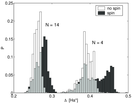
Figure 8: Addition-energy distributions for two quantum dots of 4 and 14 interacting electrons, respectively. The results have beed calculated both by (i) taking all the possible ground-state spins into account (dark gray) and (ii) neglecting Hund’s rule and thus setting $S=0$ and $1/2$ for the ground states of $N=4,14$ and $N=3,5,13,15$, respectively (white).

shows the addition-energy distributions for $N=4$ and $14$ QD’s when the different ground-state spins are included (dark grey) and neglected (white). With both $N$, there is (approximately) an equal possibility for $S=1$ ($\sim$ clean) and $S=0$ (distorted), leading to a larger width of the distribution. When $N=4$, the splitting of the different spin states into two separate peaks is clear. Hence, the measured addition energy may depend strongly on the impurity configuration of the particular sample.

Fractions of $S=0$ and $S=1$ ground states in the calculated configurations for even $N$ are shown in Table 1. Except a few results in $N=12$ QD and $\sim 1\,\%$ of the configurations in $N=20$ QD, the magic electron numbers correspond to $S=0$ states. Otherwise, the $S=1$ states formed by Hund’s rule are dominant. The $N=16$ QD, which in the clean case has a half-filled shell with a four-fold degeneracy, has also a significant fraction of $S=2$ states.

We underline that due to the primarily parabolic confining potential and a relatively small number of impurities, the shell structure is generally a dominating feature in the energetics. However, the features of disorder are clearly visible in the results: (i) A considerable fraction of the configurations shows Wigner shape in the level-spacing distribution (Fig. 5); (ii) the relative fluctuation in $\left<\Delta\right>$ is largest for filled-shell QD’s; (iii) interactions bring Gaussian contribution to the distribution functions in the mid-shell regime (Fig. 8). The last feature is typical for chaotic and disordered QD’s with considerable electron-electron interactions. berkovits

VI Summary

To summarize, we have used a fast response-function algorithm within the spin-density-functional theory to study the stability of the shell structure in few-electron quantum dots. A single impurity near the quantum dot may cause dramatic changes in the addition energies, but the shell structure is generally preserved with high peaks at the magic electron numbers. The same effect was found using a model of one thousand random impurity configurations, even if the fluctuations are largest in the filled-shell regime. In the noninteracting picture, the addition-energy distributions are combinations of Poisson and Wigner forms. The electron-electron interactions induce a shift to higher energies and considerably smaller fluctuations. In the mid-shell regime, changes in the ground-state spin lead to a strong broadening of the distribution. Hence, in a series of measurements there can be large fluctuations in those addition energies, and the result for a particular quantum dot strongly depends on the impurities in the sample.

- (1) For a review, see, e.g., L. P. Kouwenhoven, D. G. Austing, and S. Tarucha, Rep. Prog. Phys. 64, 701 (2001); S. M. Reimann and M. Manninen, Rev. Mod. Phys. 74, 1283 (2002).
- (2) S. Tarucha, D. G. Austing, T. Honda, R. J. van der Hage, and L. P. Kouwenhoven, Phys. Rev. Lett. 77, 3613 (1996).
- (3) K. Hirose and N. S. Wingreen, Phys. Rev. B 59, 4604 (1999).
- (4) S. M. Reimann, M. Koskinen, J. Kolehmainen, M. Manninen, D. G. Austing, and S. Tarucha, Eur. Phys. J. D 9, 105 (1999).
- (5) P. Matagne, J. P. Leburton, D. G. Austing, and S. Tarucha, Phys. Rev. B 65, 085325 (2002).
- (6) R. C. Ashoori, H. L. Stormer, J. S. Weiner, L. N. Pfeiffer, S. J. Pearton, K. W. Baldwin, and K. W. West, Phys. Rev. Lett. 68, 3088 (1992).
- (7) E. Räsänen, J. Könemann, R. J. Haug, M. J. Puska, and R. M. Nieminen, Phys. Rev. B 70, 115308 (2004).
- (8) V. Halonen, P. Hyvönen, P. Pietiläinen, and T. Chakraborty, Phys. Rev. B 53, 6971 (1996).
- (9) K. Hirose, F. Zhou, and N. S. Wingreen, Phys. Rev. B 63, 75301 (2001).
- (10) A. D. Güçlü, J. S. Wang, and H. Guo, Phys. Rev. B 68, 035304 (2003).
- (11) K. Hirose and N. S. Wingreen, Phys. Rev. B 65, 193305 (2002).
- (12) U. Sivan, R. Berkovits, Y. Aloni, O. Prus, A. Auerbach, and G. Ben-Yoseph, Phys. Rev. Lett. 77, 1123 (1996).
- (13) R. Berkovits, Phys. Rev. Lett. 81, 2128 (1998).
- (14) M. Aichinger and E. Krotscheck, submitted to Comp. Phys. Comm.
- (15) With our material parameters, the effective Hartree meV and the effective Bohr radius nm.
- (16) C. Attaccalite, S. Moroni, P. Gori-Giorgi, and G. B. Bachelet, Phys. Rev. Lett. 88, 256601 (2002).
- (17) J.Auer and E. Krotscheck, Comp. Phys. Comm. 118, 139 (1999).
- (18) J. Auer and E. Krotscheck, Comp. Phys. Comm. 151, 265 (2003).
- (19) J. Auer, E. Krotscheck, and S. A. Chin, J. Chem. Phys. 115, 6841 (2001).
- (20) D. Pines and P. Nozieres, The theory of quantum liquids (Benjamin, New York, 1966).
- (21) D. J. Thouless, The quantum mechanics of many-body systems, 2 ed. (Academic Press, New York, 1972).
- (22) R. P. Feynman, Phys. Rev. 94, 262 (1954).
- (23) T. Chakraborty and P. Pietiläinen, Phys. Rev. B 50, 8460 (1994).
- (24) M. Koskinen, M. Manninen, and S. M. Reimann, Phys. Rev. Lett. 79, 1389 (1997).
- (25) A. Harju, E. Räsänen, H. Saarikoski, M. J. Puska, R. M. Nieminen, and K. Niemelä, Phys. Rev. B 69, 153101 (2004).
- (26) H.-J. Stockmann, Quantum Chaos: An Introduction (Cambridge University Press, Cambridge, 2000).