Non-equilibrium temperatures in steady-state systems with conserved energy

Abstract

We study a class of non-equilibrium lattice models describing local redistributions of a globally conserved quantity, which is interpreted as an energy. A particular subclass can be solved exactly, allowing to define a statistical temperature $T_{th}$ along the same lines as in the equilibrium microcanonical ensemble. We compute the response function and find that when the fluctuation-dissipation relation is linear, the slope $T_{FD}^{-1}$ of this relation differs from the inverse temperature $T_{th}^{-1}$. We argue that $T_{th}$ is physically more relevant than $T_{FD}$, since in the steady-state regime, it takes equal values in two subsystems of a large isolated system. Finally, a numerical renormalization group procedure suggests that all models within the class behave similarly at a coarse-grained level, leading to a new parameter which describes the deviation from equilibrium. Quantitative predictions concerning this parameter are obtained within a mean-field framework.

I Introduction

The existence and the precise definition of intensive thermodynamical parameters in out-of-equilibrium systems still remains an open issue. Indeed, the goal of a statistical approach for non-equilibrium systems, which remains to be constructed, would be to give a well-defined meaning to such thermodynamical parameters, and to predict their relation with extensive macroscopic variables like energy or volume. Accordingly, many attempts have been made to define out-of-equilibrium temperatures in the last decades Jou .

In the context of glasses, which are non-stationary systems with very large relaxation times, effective temperatures have been first introduced as phenomenological parameters allowing to account for experimental data Tool ; Naraya ; Moynihan . More recently, the notion of effective temperature has been given a more fundamental status, being defined as the inverse of the slope of fluctuation-dissipation relations (FDR) in the aging regime CuKuPe . This definition was guided by the dynamical results obtained within a family of mean-field spin glass models CuKu . Interestingly, such a definition of the effective temperature has been shown to satisfy the basic properties expected for a temperature CuKuPe . Since then, a lot of numerical simulations Parisi ; Kob ; Barrat00 ; Sciortino ; Berthier ; Zamponi ; Ritort and experiments Israeloff ; Ciliberto ; Ocio ; Danna ; Abou have been conducted to test the validity of this definition of temperature in the aging regime of glassy materials. Yet, this definition seems not to be always applicable as the measured FDR can be non linear.

Other classes of systems are far from equilibrium not due to their slow relaxation towards the equilibrium state, but rather because they are subjected to external constraints producing fluxes (of particles or energy for example) traversing the system, leading to energy dissipation. As a result, they never reach an equilibrium state. Among these systems, one can think of granular gases, sheared fluid or certain kinetic spin models, to quote only a few of them.

Although the usual formalism of equilibrium statistical physics does not apply to these systems, it is interesting to note that the latter sometimes share with equilibrium systems some quantitative properties, like critical behavior Grinstein ; Tauber . To describe the statistical properties of such non-equilibrium systems, effective temperatures have been defined either from FDR Baldassarri ; Barrat03 ; Chate or from maximum entropy conditions Chate ; Miller , as originally proposed by Jaynes Jaynes . Still, the validity of these procedures remains to be clarified in the context of non glassy out-of-equilibrium systems.

When described in a probabilistic language, a common feature of these systems is that they do not obey the detailed balance property, considered as a signature of equilibrium dynamics. Since the breaking of detailed balance plays an important role in non-equilibrium systems, it may be useful to distinguish between different forms of detailed balance which should not be confused. In the literature, the term ‘detailed balance’ often refers to a canonical form which reads:

$$W(\beta|\alpha)\,e^{-E_{\alpha}/T}=W(\alpha|\beta)\,e^{-E_{\beta}/T}$$ (1)

where $W(\beta|\alpha)$ is the transition rate from state $\alpha$ to state $\beta$. This criterion on transition rates ensures that the statistical equilibrium reached at large times by the system is indeed the canonical equilibrium at temperature $T$.

Still, the above approach requires to know the equilibrium distribution before defining the stochastic model. On the contrary, one could try to find a stochastic model which describes in the best possible way a given complex hamiltonian system, without knowing a priori the equilibrium distribution. Such a stochastic model should at least preserve the symmetries of the original hamiltonian system, which are the energy conservation and the time-reversal symmetry $t\to-t$ (additional symmetries –translation, rotation, etc.– must be taken also into account when present). Energy conservation is easily implemented in the stochastic rules by allowing only transitions between states with the same energy. On the other side, the time-reversal symmetry in the hamiltonian system can be interpreted in a stochastic language as the equality between two opposit transition rates: $W(\beta|\alpha)=W(\alpha|\beta)$, a property called microcanonical detailed balance or microreversibility.

In the context of non-equilibrium systems, one expects that the time-reversal symmetry is broken due to the presence of fluxes or dissipation. Hence, a simple way to define a non-equilibrium system is to consider more general microcanonical forms of detailed balance relations such as:

$$W(\beta|\alpha)f_{\alpha}=W(\alpha|\beta)f_{\beta}$$ (2)

where $f_{\alpha}$ is the statistical weight of state $\alpha$, and with $E_{\alpha}=E_{\beta}$.

In this paper, we study a class $\mathcal{C}$ of non-equilibrium lattice models describing local redistributions of a globally conserved quantity, which is interpreted as an energy. A particular subclass $\mathcal{C}_{s}$ satisfies a microcanonical detailed balance relation of the form (2), which differs from microreversibility and can be solved exactly, allowing to define a statistical temperature $T_{th}$ along the same lines as in the equilibrium microcanonical ensemble. The response function is computed explicitely, and the FDR is found to be linear or non linear depending on the model considered –the response can even be non linear with the perturbing field. Very interestingly, when the FDR is linear, its slope differs from the inverse temperature $T_{th}^{-1}$, which questions the relevance of FDR to define a temperature in non glassy out-of-equilibrium systems. Finally, we implement numerically a functional renormalization group procedure to argue that all the models within the class $\mathcal{C}$ behave at the coarse-grained level as a member of the subclass $\mathcal{C}_{s}$. Predictions about the renormalization procedure are also made using mean-field arguments, and are quantitatively verified. Note that a short version of some aspects of this work has appeared in court , and that a related model, including kinetic constraints, has also been introduced in the context of glassy dynamics Lequeux .

II Models and steady-state properties

II.1 Definition

The models we consider in this paper are defined as follows. On each site $i$ of a $d$-dimensional lattice, a real variable $x_{i}$ which can take either positive or negative values is introduced. Dynamical rules are defined such that the quantity

$$E=\sum_{i=1}^{N}g(x_{i})$$ (3)

is conserved. The function $g(x)$, assumed to be positive with continuous derivative, decreases for $x<x_{0}$ and increases for $x>x_{0}$, where $x_{0}$ is an arbitrary given value. Without loss of generality, we assume $g(x_{0})=0$. Quite importantly, the steady-state distribution can be computed with these hypotheses only. However, to clarify the presentation, we assume in this section that $x_{0}=0$ and $g(x)$ is an even function of $x$.

It is also necessary to introduce the reciprocal function $g^{-1}(y)$, given as the positive root of the equation $g(x)=y$. The dynamics is defined as follows: at each time step, a link $(j,k)$ is randomly chosen on the lattice and the corresponding variables $x_{j}$ and $x_{k}$ are updated so as to conserve the energy $g(x_{j})+g(x_{k})$ of the link. To be more specific, the new values $x_{j}^{\prime}$ and $x_{k}^{\prime}$ are given by

$$x_{j}^{\prime}=\pm g^{-1}(qS_{jk})\qquad x_{k}^{\prime}=\pm g^{-1}((1-q)S_{jk})$$ (4)

with $S_{jk}\equiv g(x_{j})+g(x_{k})$, and $q$ is a random variable drawn from a distribution $\psi(q)$, assumed to be symmetric with respect to $q=\frac{1}{2}$ ($0<q<1$). The new values $x_{j}^{\prime}$ and $x_{k}^{\prime}$ are either positive or negative with equal probability, and without correlation between the signs. Thus a model belonging to this class is characterized by two functions $g(x)$ and $\psi(q)$.

II.2 Master equation

The system is described by the distribution $P(\{x_{i}\},t)$, which gives the probability to be in a configuration $\{x_{i}\}$ at time $t$. Its evolution is given by the master equation:

$$\frac{\partial P}{\partial t}(\{x_{i}\},t) = \int\prod_{i}dx_{i}^{\prime}\,W(\{x_{i}\}|\{x_{i}^{\prime}\})\,P(\{x_{i}^{\prime}\},t)$$

$$\quad-\int\prod_{i}dx_{i}^{\prime}\,W(\{x_{i}^{\prime}\}|\{x_{i}\})\,P(\{x_{i}\},t)$$

where $W(\{x_{i}^{\prime}\}|\{x_{i}\})$ is the transition rate from configuration $\{x_{i}\}$ to configuration $\{x_{i}^{\prime}\}$. The transition rate can be decomposed into a sum over the links of the lattice:

$$W(\{x_{i}^{\prime}\}|\{x_{i}\})=\sum_{\langle j,k\rangle}W_{jk}(\{x_{i}^{\prime}\}|\{x_{i}\})$$ (6)

where $W_{jk}(\{x_{i}^{\prime}\}|\{x_{i}\})$ accounts for the redistribution over a given link $(j,k)$:

$$W_{jk}(\{x_{i}^{\prime}\}|\{x_{i}\})=\left[\prod_{i\neq j,k}\delta(x_{i}^{\prime}-x_{i})\right]\int_{0}^{1}dq\,\psi(q)\times$$ (7)

$$\>\frac{1}{4}\sum_{\sigma_{j},\sigma_{k}}\delta\left[x_{j}^{\prime}-\sigma_{j}g^{-1}(qS_{jk})\right]\,\delta\left[x_{k}^{\prime}-\sigma_{k}g^{-1}((1-q)S_{jk})\right]$$

where the variables $\sigma_{j}$, $\sigma_{k}=\pm 1$ account for the random signs appearing in Eq. (4) with probability $\frac{1}{2}$ –hence the factor $\frac{1}{4}$ in the above equation. After some algebra, the transition rate $W(\{x_{i}^{\prime}\}|\{x_{i}\})$ can be rewritten as:

$$W(\{x_{i}^{\prime}\}|\{x_{i}\})=\frac{1}{4}\sum_{\langle j,k\rangle}\left[\prod_{i\neq j,k}\delta(x_{i}^{\prime}-x_{i})\right]\,\times$$ (8)

$$\quad\frac{|g^{\prime}(x_{j}^{\prime})g^{\prime}(x_{k}^{\prime})|}{S_{jk}}\,\psi\left(\frac{g(x_{j}^{\prime})}{S_{jk}}\right)\delta\left[g(x_{j}^{\prime})+g(x_{k}^{\prime})-S_{jk}\right]$$

where $g^{\prime}(x)$ denotes the derivative of $g(x)$.

II.3 Detailed balance and steady-state distribution

A case of particular interest is the subclass of models for which the distribution $\psi(q)$ is given by a symmetric beta law:

$$\psi(q)=\frac{\Gamma(2\eta)}{\Gamma(\eta)^{2}}\,q^{\eta-1}(1-q)^{\eta-1}$$ (9)

with $\eta>0$. In this case, the function $\psi(g(x_{j}^{\prime})/S_{jk})$ appearing in the transition rates factorizes, if one takes into account the delta function. So the transition rate reads

$$W(\{x_{i}^{\prime}\}|\{x_{i}\})=\frac{\Gamma(2\eta)}{4\Gamma(\eta)^{2}}\;\sum_{\langle j,k\rangle}\left[\prod_{i\neq j,k}\delta(x_{i}^{\prime}-x_{i})\right]\times$$ (10)

$$\frac{|g^{\prime}(x_{j}^{\prime})g^{\prime}(x_{k}^{\prime})|}{S_{jk}^{2\eta-1}}\,g(x_{j}^{\prime})^{\eta-1}g(x_{k}^{\prime})^{\eta-1}\delta\left[g(x_{j}^{\prime})+g(x_{k}^{\prime})-S_{jk}\right]$$

From this last expression, it can be checked that a detailed balance relation is satisfied:

$$W(\{x_{i}^{\prime}\}|\{x_{i}\})\,\prod_{i=1}^{N}\left[|g^{\prime}(x_{i})|\,g(x_{i})^{\eta-1}\right]=$$ (11)

$$\qquad\qquad W(\{x_{i}\}|\{x_{i}^{\prime}\})\,\prod_{i=1}^{N}\left[|g^{\prime}(x_{i}^{\prime})|\,g(x_{i}^{\prime})^{\eta-1}\right]$$

As a result, the steady-state distribution $P_{st}(\{x_{i}\}|E)$, for a given value $E$ of the energy, is readily obtained as:

$$P_{st}(\{x_{i}\}|E) = \frac{1}{Z_{N}(E)}\,\prod_{i=1}^{N}\left[|g^{\prime}(x_{i})|\,g(x_{i})^{\eta-1}\right]\times$$

$$\qquad\qquad\qquad\quad\delta\left(\sum_{i=1}^{N}g(x_{i})-E\right)$$

where $Z_{N}(E)$ is a normalization factor that may be called an effective (microcanonical) partition function:

$$Z_{N}(E) = \int\prod_{i=1}^{N}\left[dx_{i}\,|g^{\prime}(x_{i})|\,g(x_{i})^{\eta-1}\right]\times$$

$$\qquad\qquad\qquad\quad\delta\left(\sum_{i=1}^{N}g(x_{i})-E\right)$$

An important remark has to be made at this stage: Eqs. (II.3) and (II.3) remain formally valid if one slightly changes the definition of the model. This can be done in two different ways. First, one could consider the case where the variables $\{x_{i}\}$ take only positive values. Then one only needs to remove the sum $\frac{1}{4}\sum_{\sigma_{j},\sigma_{k}}$ in the transition rates given in Eq. (7), and Eq. (II.3) is recovered, with this time $x_{i}>0$. Second, as mentioned in Sect. II.1, the model can be generalized by assuming that $g(x)$ is not an even function. This is particularly useful if one wants to include an external field which breaks the $+/-$ symmetry –see Sect. III.2. Actually, if $g(x)$ decreases for $x<x_{0}$, and increases for $x>x_{0}$, the distribution given in Eq. (II.3) also holds .

The function $Z_{N}(E)$ can be computed using a Laplace transform. Indeed, it appears rather clearly from Eq. (II.3), by making the change of variable $\varepsilon_{i}=g(x_{i})$, that $Z_{N}(E)$ is actually independent of the functional form of $g(x)$. One finds

$$Z_{N}(E)=\kappa_{N}\,E^{\eta N-1}$$ (14)

with $\kappa_{N}=2^{N}\,\Gamma(\eta)^{N}/\Gamma(\eta N)$. The fact that $Z_{N}(E)$ does not depend on $g(x)$ is actually not a coincidence, but comes from the basic definition of the model given in Eq. (4). Indeed, for any function $g(x)$, one could choose as the dynamical variables the local energies $\varepsilon_{i}=g(x_{i})$, and solve the model for $\varepsilon_{i}$. Coming back to the variable $g(x_{i})$ at the end of the calculations, the distribution (II.3) would be recovered. Still, it should not be concluded from this that all physical quantities defined in the model are independent of $g(x)$. In particular, the response to a perturbing field depends strongly on $g(x)$, since the field is coupled to $x$, and not to the energy $g(x)$ –see Sect. III.2.

An interesting question is also to see under what conditions microreversibility (to be associated to the equilibrium behavior) can be recovered in this model. Microreversibility holds if $|g^{\prime}(x)|\,g(x)^{\eta-1}$ is independent of $x$, as can be seen from Eq. (II.3). Such a condition can be satisfied only if $g(x)$ is a power law, say $g(x)=x^{p}/p$, where $p$ is an even integer to ensure the regularity of $g(x)$ around $x=0$. The factor $1/p$ has been added for convenience, but is otherwise arbitrary. One then has

$$|g^{\prime}(x)|\,g(x)^{\eta-1}=p^{1-\eta}\,|x|^{\eta p-1}$$ (15)

Accordingly, microreversibility is recovered for $\eta=1/p$. On the contrary, for $\eta\neq 1/p$, significant differences with the equilibrium behavior are expected. These differences may be even stronger if $g(x)$ is not a power law.

III Non-equilibrium temperatures

III.1 Statistical approach

III.1.1 Microcanonical equilibrium

In order to define a temperature in this model, one can try to follow a procedure similar to that of the microcanonical ensemble in equilibrium statistical physics. Indeed, one of the main motivations when building the present model was to find a model in which a global quantity (the energy) is conserved, so as to ‘mimic’ in some sense a microcanonical situation. Yet, as mentioned above, the absence of microreversibility should yield important differences with the latter case. For an equilibrium system in the microcanonical ensemble, temperature is introduced in the following way. Considering a large system $\mathcal{S}$ with fixed energy, one introduces a partition into two subsystems $\mathcal{S}_{1}$ and $\mathcal{S}_{2}$, with energy $E_{\ell}$ and a number $N_{\ell}$ of degrees of freedom ($\ell=1,2$). These two subsystems are no longer isolated, since they can mutually exchange energy; the only constraint is that $E_{1}+E_{2}=E$ is fixed. The key quantity is then the number $\Omega_{N_{\ell}}(E_{\ell})$ of accessible states with energy $E_{\ell}$ in the subsystem $\mathcal{S}_{\ell}$; in systems with continuous degrees of freedom (like a classical gas for instance), $\Omega_{N_{\ell}}(E_{\ell})$ is the area of the hypersurface of energy $E_{\ell}$ in phase space. Assuming that both subsystems do not interact except by exchanging energy, the number of states of the system $\mathcal{S}$ compatible with the partition $(E_{1},E_{2})$ of the energy is equal to $\Omega_{N_{1}}(E_{1})\Omega_{N_{2}}(E_{2})$. But since $E_{1}+E_{2}$ is fixed, the most probable value $E_{1}^{*}$ is found from the maximum, with respect to $E_{1}$, of $\Omega_{N_{1}}(E_{1})\Omega_{N_{2}}(E-E_{1})$. Taking a logarithmic derivative, one finds the usual result:

$$\frac{\partial\ln\Omega_{N_{1}}}{\partial E_{1}}\Big{|}_{E_{1}^{*}}=\frac{\partial\ln\Omega_{N_{2}}}{\partial E_{2}}\Big{|}_{E-E_{1}^{*}}$$ (16)

Defining the microcanonical temperature $T_{\ell}$ of subsystem $\ell$ by the relation

$$\frac{1}{T_{\ell}}=\frac{\partial\ln\Omega_{N_{\ell}}}{\partial E_{\ell}}\Big{|}_{E_{\ell}^{*}}$$ (17)

one sees from Eq. (16) that $T_{1}=T_{2}$, i.e. that the temperatures are equal in both subsystems (throughout the paper, the Boltzmann constant $k_{B}$ is set to unity). In addition, it can also be shown that the common value $T$ does not depend on the partition chosen; as a result, $T$ is said to characterize the full system $\mathcal{S}$.

III.1.2 ‘Microcanonical’ stationary state

Very interestingly, this microcanonical definition of temperature can be generalized in a rather straightforward way to the present model. Still, it should be noticed first that microscopic configurations compatible with the given value of the energy are no longer equiprobable, as seen from the distribution (II.3), so that $\Omega_{N}(E)$ is no more relevant to the problem. But starting again from a partition into two subsystems as above, one can determine the most probable value $E_{1}^{*}$ from the maximum of the conditional probability $P(E_{1}|E)$ that subsystem $\mathcal{S}_{1}$ has energy $E_{1}$ given that the total energy is $E$. Indeed, in the equilibrium case, $P(E_{1}|E)$ reads

$$P(E_{1}|E)=\frac{\Omega_{N_{1}}(E_{1})\,\Omega_{N_{2}}(E-E_{1})}{\Omega_{N}(E)}$$ (18)

which by derivation with respect to $E_{1}$, yields precisely the same result as Eq. (16).

To be more specific, the subsystems are defined in the present model as a partition of the lattice, with $N_{1}$ sites in $\mathcal{S}_{1}$ and $N_{2}$ sites in $\mathcal{S}_{2}$. The conditional distribution $P(E_{1}|E)$ is then given by:

$$P(E_{1}|E) = \int\prod_{i=1}^{N}dx_{i}\,P_{st}(\{x_{i}\}|E)\,\delta\left(\sum_{i\in\mathcal{S}_{1}}g(x_{i})-E_{1}\right)$$

$$= \frac{1}{Z_{N}(E)}\int\prod_{i=1}^{N}\left[dx_{i}\,|g^{\prime}(x_{i})|\,g(x_{i})^{\eta-1}\right]\times$$

$$\quad\delta\left(\sum_{i=1}^{N}g(x_{i})-E\right)\,\delta\left(\sum_{i\in\mathcal{S}_{1}}g(x_{i})-E_{1}\right)$$

Taking into account the last delta function, the first one can be replaced by $\delta(\sum_{i\in\mathcal{S}_{2}}g(x_{i})-(E-E_{1}))$, so that $P(E_{1}|E)$ may be written in a compact form as:

$$P(E_{1}|E)=\frac{Z_{N_{1}}(E_{1})\,Z_{N_{2}}(E-E_{1})}{Z_{N}(E)}$$ (20)

This result generalizes in a nice way the equilibrium distribution Eq. (18), since in equilibrium $Z_{N}(E)$ reduces precisely to $\Omega_{N}(E)$. The most probable value $E_{1}^{*}$ satisfies

$$\frac{\partial\ln P(E_{1}|E)}{\partial E_{1}}\Big{|}_{E_{1}^{*}}=0$$ (21)

which yields

$$\frac{\partial\ln Z_{N_{1}}}{\partial E_{1}}\Big{|}_{E_{1}^{*}}=\frac{\partial\ln Z_{N_{2}}}{\partial E_{2}}\Big{|}_{E-E_{1}^{*}}$$ (22)

So in close analogy with the equilibrium approach, we define a temperature $T_{th}^{\ell}$ for subsystem $\mathcal{S}_{\ell}$ through

$$\frac{1}{T_{th}^{\ell}}=\frac{\partial\ln Z_{N_{\ell}}}{\partial E_{\ell}}\Big{|}_{E_{\ell}^{*}}$$ (23)

Then Eq. (22) implies that $T_{th}^{1}=T_{th}^{2}$.

At this stage, it is important to check that the common value $T_{th}$ of the temperature does not depend on the partition chosen. To this aim, we show that $T_{th}$ can be expressed as a function of global quantities characterizing the whole system, with no reference to the specific partition.

Let us compute $Z_{N}(E)$ as a function of $Z_{N_{1}}(E_{1})$ and $Z_{N_{2}}(E_{2})$. Since $\int_{0}^{E}dE_{1}\,P(E_{1}|E)=1$, one has from Eq. (20):

$$Z_{N}(E)=\int_{0}^{E}dE_{1}\,Z_{N_{1}}(E_{1})\,Z_{N_{2}}(E-E_{1})$$ (24)

We assume the following general scaling form at large $N_{\ell}$ for $Z_{N_{\ell}}(E_{\ell})$:

$$Z_{N_{\ell}}(E_{\ell})=A_{\ell}\,\exp[N_{\ell}\zeta_{\ell}(\overline{\varepsilon}_{\ell})]$$ (25)

with $\overline{\varepsilon}_{\ell}\equiv E_{\ell}/N_{\ell}$ (the index $\ell=1,2$ labels the subsystem). This scaling form is demonstrated explicitely in Sect. III.1.3. Using a saddle-point calculation, one obtains for $Z_{N}(E)$ a relation of the form (with $\overline{\varepsilon}=E/N$):

$$Z_{N}(E)=Z_{N_{1}}(E_{1}^{*})\,Z_{N_{2}}(E_{2}^{*})\,N\int_{0}^{\overline{\varepsilon}}d\varepsilon_{1}\,e^{-N\,b(\overline{\varepsilon})\,(\varepsilon_{1}-\overline{\varepsilon}_{1}^{*})^{2}}$$ (26)

where $b(\overline{\varepsilon})$ is defined as:

$$b(\overline{\varepsilon})=-\frac{1}{2}\left[\lambda_{1}\zeta_{1}^{\prime\prime}(\overline{\varepsilon}_{1}^{*})+\lambda_{2}\zeta_{2}^{\prime\prime}(\overline{\varepsilon}-\overline{\varepsilon}_{1}^{*})\right]$$ (27)

with $\lambda_{\ell}=N_{\ell}/N$. Thus $\ln Z_{N}(E)$ reads:

$$\ln Z_{N}(E)=\ln Z_{N_{1}}(E_{1}^{*})+\ln Z_{N_{2}}(E-E_{1}^{*})-\frac{1}{2}\ln b(\overline{\varepsilon})+C$$ (28)

where $C$ does not depend on $E$. Taking the derivative with respect to $E$ yields, using Eq. (23):

$$\frac{\partial\ln Z_{N}}{\partial E}=\frac{1}{T_{th}}\,\frac{\partial E_{1}^{*}}{\partial E}+\frac{1}{T_{th}}\,\left(1-\frac{\partial E_{1}^{*}}{\partial E}\right)-\frac{1}{2N}\,b^{\prime}(\overline{\varepsilon})$$ (29)

In the limit $N\to\infty$ (with $\overline{\varepsilon}$ fixed), the last term vanishes, whereas $T_{th}$ has a finite limit due to the scaling form Eq. (25), so that

$$\frac{\partial\ln Z_{N}}{\partial E}=\frac{1}{T_{th}}$$ (30)

As a result, $T_{th}$ can be computed from the global quantity $Z_{N}(E)$ instead of $Z_{N_{1}}(E_{1})$ or $Z_{N_{2}}(E_{2})$, and is thus independent of the partition chosen. This temperature characterizes the statistical state of the whole system. From Eq. (14), the equation of state of the system is:

$$E=\eta NT_{th}$$ (31)

In the case of a quadratic energy, i.e. $g(x)=\frac{1}{2}x^{2}$, it has been shown above that the equilibrium behavior is recovered for $\eta=\frac{1}{2}$. This result is confirmed by Eq. (31), which reduces for $\eta=\frac{1}{2}$ to the usual form of the energy equipartition. On the contrary, for $\eta\neq\frac{1}{2}$, a generalized form of equipartition holds in the sense that all the sites have the same average energy $\overline{\varepsilon}=E/N$ (which is not surprising given the homogeneity of the system), but this average energy per degree of freedom is equal to $\eta T_{th}$ instead of $\frac{1}{2}T_{th}$. This point will be discussed in more details later on.

Up to now, we have considered only the ‘microcanonical’ (in a generalized sense) distribution $P_{st}(\{x_{i}\}|E)$. Yet, it would be interesting to introduce also the analogous of the canonical distribution. To do so, we compute the distribution $P_{can}(\{x_{i}\})$ associated to a small (but still macroscopic) subsystem $\mathcal{S}_{1}$ of a large isolated system $\mathcal{S}$. The degrees of freedom $\{x_{i}\}$ with $i=N_{1}+1,\ldots,N$ have to be integrated out since they belong to the reservoir. One finds for the remaining $\{x_{i}\}$ ($i=1,\ldots,N_{1}$) the following distribution:

$$P_{can}(\{x_{i}\})=\frac{1}{Z_{N}(E)}\prod_{i=1}^{N_{1}}|g^{\prime}(x_{i})|\ g(x_{i})^{\eta-1}\times$$ (32)

$$\int\prod_{i=N_{1}+1}^{N}\left[dx_{i}\,|g^{\prime}(x_{i})|\,g(x_{i})^{\eta-1}\right]\,\delta\left(\sum_{i=1}^{N}g(x_{i})-E\right)$$

The above integral is nothing but the partition function $Z_{N_{2}}(E-\sum_{i=1}^{N_{1}}g(x_{i}))$, with $N_{2}=N-N_{1}$, which can be expanded to first order as:

$$\ln Z_{N_{2}}\left(E-\sum_{i=1}^{N_{1}}g(x_{i})\right)=\ln Z_{N_{2}}(E)-\frac{1}{T_{th}}\sum_{i=1}^{N_{1}}g(x_{i})$$ (33)

assuming that $\sum_{i=1}^{N_{1}}g(x_{i})\ll E$, which is true as long as $N_{1}\ll N$. The derivative of $\ln Z_{N_{2}}(E)$ has been identified with $1/T_{th}$ using Eq. (23), up to corrections that vanish in the limit $N_{1}/N\to 0$, since $E$ is the total energy rather than the energy $E_{2}$ of the reservoir. Introducing this last result into Eq. (32), one finally finds

$$P_{can}(\{x_{i}\}) = \frac{1}{Z_{N_{1}}^{can}}\,\prod_{i=1}^{N_{1}}|g^{\prime}(x_{i})|\,g(x_{i})^{\eta-1}\times$$

$$\qquad\qquad\exp\left(-\frac{1}{T_{th}}\sum_{i=1}^{N_{1}}g(x_{i})\right)$$

where $Z_{N_{1}}^{can}=Z_{N_{2}}(E)/Z_{N}(E)$ –note that $E$ is the energy of the global system which includes the reservoir. This ‘canonical’ distribution appears to be useful in order to compute the FDR, as discussed below in Sect. III.2.

III.1.3 Entropy and thermodynamics

From Eq. (30), it is tempting to generalize the notion of microcanonical entropy through $S(E)=\ln Z_{N}(E)$. Indeed, this definition is not only an analogy, but as we shall see, it can be associated with a time-dependent entropy which is maximized by the dynamics. To define the entropy, one needs first to introduce the probability measure $P_{E}(\{x_{i}\},t)$ restricted to the hypersurface of energy $E$:

$$P(\{x_{i}\},t)=P_{E}(\{x_{i}\},t)\;\delta\left(\sum_{i=1}^{N}g(x_{i})-E\right)$$ (35)

Then the dynamical entropy is defined as:

$$S_{E}(t)=-\int\prod_{i=1}^{N}dx_{i}\,P(\{x_{i}\},t)\,\ln\frac{P_{E}(\{x_{i}\},t)}{f(\{x_{i}\})}$$ (36)

where $f(\{x_{i}\})\equiv\prod_{i=1}^{N}|g^{\prime}(x_{i})|\,g(x_{i})^{\eta-1}$. Using the master equation (II.2), it can be shown that $S_{E}(t)$ is a non-decreasing function of time –see Appendix A. As a result, $S_{E}(t)$ is maximal in the stationary state, and the corresponding value $S(E)$ is given by:

$$S(E) = -\int\prod_{i=1}^{N}dx_{i}\,P(\{x_{i}\}|E)\,\ln\frac{1}{Z_{N}(E)}$$ (37)

$$= \ln Z_{N}(E)$$

which matches exactly the definition proposed above on the basis of Eq. (30).

Using Eq. (14), one can compute $S(E)$ and check explicitely that the entropy per site $S(E)/N$ becomes in the thermodynamic limit a well-defined function $\zeta(\overline{\varepsilon})$ of the energy density $\overline{\varepsilon}=E/N$. The entropy $S(E)$ reads:

$$S(E)=N\left[\ln 2\Gamma(\eta)-\frac{1}{N}\ln\Gamma(\eta N)+\eta\ln E\right]$$ (38)

As $\ln\Gamma(x)\approx x\ln x-x$ for large $x$, one finds:

$$\frac{1}{N}\ln\Gamma(\eta N)\approx\eta(\ln\eta-1)+\eta\ln N$$ (39)

which allows to write $S(E)=N\zeta(\overline{\varepsilon})$ with:

$$\zeta(\overline{\varepsilon})=\eta\ln\overline{\varepsilon}+\ln 2\Gamma(\eta)-\eta(\ln\eta-1)$$ (40)

On the other hand, the equilibrium thermodynamic formalism is most often formulated in terms of the canonical ensemble. In the present model, since a canonical distribution has been derived, it may also be possible to define an equivalent of the canonical thermodynamic formalism. Indeed, from Eq. (III.1.2), one can easily see that the average energy $\langle E\rangle$ is given by

$$\langle E\rangle=-\frac{\partial\ln Z_{N}^{can}}{\partial\beta}$$ (41)

where $\beta\equiv T_{th}^{-1}$ is the inverse temperature. A generalized free energy $F(T_{th})$ is also naturally introduced through

$$F(T_{th})=-T_{th}\ln Z_{N}^{can}$$ (42)

The generalized partition function $Z_{N}^{can}$ can be easily computed, as it is factorized:

$$Z_{N}^{can} = \left[\int_{-\infty}^{\infty}dx\,|g^{\prime}(x)|\,g(x)^{\eta-1}e^{-g(x)/T_{th}}\right]^{N}$$ (43)

$$= \left[2\int_{0}^{\infty}d\varepsilon\,\varepsilon^{\eta-1}\,e^{-\varepsilon/T_{th}}\right]^{N}$$

which leads to

$$Z_{N}^{can}=\left(2\Gamma(\eta)T_{th}^{\eta}\right)^{N}$$ (44)

So the free-energy is given by

$$F=-NT_{th}\left[\ln 2\Gamma(\eta)+\eta\ln T_{th}\right]$$ (45)

In equilibrium, the entropy $S$ is related to the free energy $F$ through

$$\frac{\partial F}{\partial T}=-S$$ (46)

This relation is also satisfied within the present model:

$$\frac{\partial F}{\partial T_{th}} = -N\left[\eta(\ln T_{th}+1)+\ln 2\Gamma(\eta)\right]$$ (47)

$$= -N\zeta(\overline{\varepsilon})$$

where the last equality is obtained by using the equation of state $T_{th}=\overline{\varepsilon}/\eta$, and comparing with Eq. (40).

III.2 Fluctuation-dissipation relations

As recalled in the introduction, temperatures are usually defined in out-of-equilibrium systems as the inverse slope of the FDR, when this relation is linear. This approach has been shown to be physically meaningful in the context of glassy models in the aging regime CuKu . In this case, the long time slope of the FDR gives an effective temperature which differs from the heat bath temperature. Still, for non-equilibrium steady-state systems which are not glassy, no justification has been proposed to show that the inverse slope of the FDR satisfies the basic properties expected for a temperature. For instance, one expects a temperature to take equal values in two subsystems of a large system, when the stationary state has been reached. The present model thus allows to test explicitely the validity of the FDR definition of temperature.

A natural observable to consider in this model is

$$M(t)=\sum_{i=1}^{N}x_{i}(t)$$ (48)

The steady-state correlation function $C(t)$ of the system is then defined as the normalized autocorrelation of the observable $M(t)$ between time $t=0$ and $t$:

$$C(t)=\frac{1}{N}\langle(M(t)-\langle M\rangle)\,(M(0)-\langle M\rangle)\rangle$$ (49)

where the brackets $\langle\dots\rangle$ denote an average over all possible trajectories of the system. Calculations are easier using the canonical distribution $P_{can}(\{x_{i}\})$; since this distribution is factorized, the random variables $x_{i}$ and $x_{j}$ are independent if $i\neq j$, so that $C(t)$ reduces to

$$C(t)=\langle(x(t)-\langle x\rangle)\,(x(0)-\langle x\rangle)\rangle$$ (50)

where $x$ stands for any of the variables $x_{i}$ –all sites have the same average values.

The aim of the FDR is to relate correlation and response of a given observable. One thus needs to introduce a perturbation which generates variations of $x$ so that a response could be defined. A simple way to perturb the system is to add to the energy a linear term proportional to an external field $h$: one then replaces $E$ by $E_{h}$ defined as:

$$E_{h}=\sum_{i=1}^{N}g_{h}(x_{i})=\sum_{i=1}^{N}g(x_{i})-hx_{i}+c_{h}$$ (51)

Without loss of generality, the new function $g_{h}(x)$ is shifted by a constant $c_{h}$ so that the minimum value of $g_{h}(x)$ remains equal to $0$. If the second derivative $g^{\prime\prime}(0)$ does not vanish, $c_{h}$ is given to leading order in $h$ by:

$$c_{h}=\frac{h^{2}}{2\,g^{\prime\prime}(0)}$$ (52)

In order to define the response function, one assumes that the system is subjected to a field $h\neq 0$ for $t<0$, and that it has reached a steady state. Then at time $t=0$, the field $h$ is switched off. The (time-dependent) response is defined for $t>0$ through:

$$\chi(t)\equiv\frac{\partial}{\partial h}\Big{|}_{h=0}\left<\frac{1}{N}\sum_{i=1}^{N}x_{i}(t)\right>_{h}$$ (53)

where the index $h$ on the brackets indicate that the average is taken over the dynamics in presence of the field $h$. The observable $\langle N^{-1}\sum_{i}x_{i}(t)\rangle_{h}$ can be computed as:

$$\left<\frac{1}{N}\sum_{i=1}^{N}x_{i}(t)\right>_{h} = \int\prod_{i=1}^{N}dx_{i}\,dx_{i}^{\prime}\,G_{t}^{0}(\{x_{i}\}|\{x_{i}^{\prime}\})\,\times$$

$$\qquad\qquad P_{can}(\{x_{i}^{\prime}\},h)\left(\frac{1}{N}\sum_{i=1}^{N}x_{i}\right)$$

where $G_{t}^{0}(\{x_{i}\}|\{x_{i}^{\prime}\})$ is the zero-field Green function, i.e. the probability for the system to be in a configuration $\{x_{i}\}$ at time $t$, given that it was in a configuration $\{x_{i}^{\prime}\}$ at time $t=0$, in the absence of field. The response function $\chi(t)$ is obtained by taking the derivative of the above equation with respect to $h$, at $h=0$:

$$\chi(t) = \int\prod_{i=1}^{N}dx_{i}\,dx_{i}^{\prime}\,G_{t}^{0}(\{x_{i}\}|\{x_{i}^{\prime}\})\,\times$$

$$\qquad P_{can}(\{x_{i}^{\prime}\},0)\,\frac{\partial\ln P_{can}}{\partial h}(\{x_{i}^{\prime}\},0)\left(\frac{1}{N}\sum_{i=1}^{N}x_{i}\right)$$

The canonical distribution $P_{can}(\{x_{i}\},h)$ in the presence of field takes the same form as Eq. (III.1.2), simply replacing $g(x)$ by $g_{h}(x)$. Thus one finds for the logarithmic derivative of $P_{can}(\{x_{i}\},h)$:

$$\frac{\partial\ln P_{can}}{\partial h}(\{x_{i}^{\prime}\},0) = -\frac{\partial\ln Z_{N}^{can}}{\partial h}\Big{|}_{h=0}\,+$$

$$\sum_{i=1}^{N}\left(\frac{x_{i}}{T_{th}}-\frac{1}{g^{\prime}(x_{i})}-(\eta-1)\frac{x_{i}}{g(x_{i})}\right)$$

Note that $dc_{h}/dh=0$ at $h=0$, due to the regularity of $g(x)$. The derivative of the partition function yields:

$$\frac{\partial\ln Z_{N}^{can}}{\partial h}\Big{|}_{h=0}=\frac{1}{T_{th}}\left<\sum_{i=1}^{N}x_{i}\right>-\left<\sum_{i=1}^{N}\omega_{i}\right>$$ (57)

where $\omega_{i}$ stands for

$$\omega_{i}\equiv\frac{1}{g^{\prime}(x_{i})}+(\eta-1)\frac{x_{i}}{g(x_{i})}$$ (58)

Replacing the expression (III.2) in Eq. (III.2), one finally finds, using the factorization of the canonical distribution:

$$\chi(t)=\frac{1}{T_{th}}\,C(t)-\langle(x(t)-\langle x\rangle)(\omega(0)-\langle\omega\rangle)\rangle$$ (59)

where indices are omitted just as in Eq. (50). Compared to the usual form of FDR, an additional term appears which corresponds to the correlation of the variables $x$ and $\omega$. In general, this new correlation function is not proportional to $C(t)$, so that a parametric plot of $\chi(t)$ versus $C(t)$, usually referred to as a fluctuation-dissipation plot, would be non linear.

Yet, in the case where $g(x)$ is an even function of $x$, some important simplifications occur. On the one hand, the average values of $x$ and $\omega$ vanish. On the other hand, the correlation $x(t)\omega(0)$ becomes proportional to the ‘hopping correlation function’ $\Phi(t)$, defined as

$$\Phi(t)=\left<\frac{1}{N}\,\sum_{i=1}^{N}\phi_{i}(t)\right>$$ (60)

The variables $\phi_{i}(t)$ are history dependent random variables, which are equal to $1$ if no redistribution involving site $i$ occured between $t=0$ and $t$, and are equal to $0$ otherwise. The proportionality of both correlation functions can be understood as follows: if there was a redistribution on site $i$ between $0$ and $t$, $x_{i}(t)$ becomes fully decorrelated from $\omega_{i}$, due to the fact that the sign of $x_{i}(t)$ is chosen at random, and that the average values $\langle x\rangle$ and $\langle\omega\rangle$ vanish for an even $g(x)$. On the contrary, if no redistribution occured, $x_{i}(t)\omega_{i}(0)=x_{i}(0)\omega_{i}(0)$. The same reasoning also holds for $C(t)$, so that one has:

$$C(t)=\langle x^{2}\rangle\,\Phi(t),\quad\langle x(t)\omega(0)\rangle=\langle x\omega\rangle\,\Phi(t)$$ (61)

As a result, the FDR can be expressed, in the case of an even function $g(x)$, as

$$\chi(t)=\left(\frac{1}{T_{th}}-\frac{\langle x\omega\rangle}{\langle x^{2}\rangle}\right)C(t)$$ (62)

So the FDR is indeed linear in this case, and one can define an effective temperature $T_{FD}$ from the inverse slope of this relation. This yields:

$$\frac{1}{T_{FD}}=\frac{1}{T_{th}}-\frac{\langle x\omega\rangle}{\langle x^{2}\rangle}$$ (63)

Still, as long as $\langle x\omega\rangle\neq 0$, the temperature $T_{FD}$ differs from the temperature $T_{th}$ defined above from statistical considerations –a more detailed discussion on this point is given below in Sect. III.3.

Even though the two temperatures are not equal, one can wonder whether they are proportional, in the sense that the ratio $T_{th}/T_{FD}$ would be independent of $T_{th}$. From Eq. (63), one has:

$$\frac{T_{th}}{T_{FD}}=1-\frac{\langle x\omega\rangle\,\langle g(x)\rangle}{\eta\,\langle x^{2}\rangle}$$ (64)

where we have used the relations $T_{th}=\overline{\varepsilon}/\eta$ and $\overline{\varepsilon}=\langle g(x)\rangle$. The correlation $\langle x\omega\rangle$ can be written in a more explicit form as

$$\langle x\omega\rangle=\left<\frac{x}{g^{\prime}(x)}+(\eta-1)\,\frac{x^{2}}{g(x)}\right>$$ (65)

From Eqs. (64) and (65), it appears that the ratio $T_{th}/T_{FD}$ generally depends on $T_{th}$, since the average $\langle\dots\rangle$ is done with the one-site distribution which is a function of temperature.

Now in the particular case where $g(x)$ is a power law, namely $g(x)=x^{p}/p$ (with $p$ an even integer), Eq. (64) actually simplifies to

$$T_{FD}=[2+p(\eta-1)]\,T_{th}$$ (66)

Note that for $2+p(\eta-1)\leq 0$, the above equation would lead to a negative $T_{FD}$, i.e. a negative response $\chi(t)$ to the perturbation $h$, which is rather counterintuitive. Actually, $\chi(t)$ does not become negative in this case but diverges and Eq. (66) is no longer valid, indicating the breakdown of linear response –the response is then non linear with $h$ even for $h\to 0$. This may be seen from the correlation $\langle x\omega\rangle$, which can be written:

$$\langle x\omega\rangle=A\int_{0}^{\infty}dx\,x^{1+p(\eta-1)}e^{-x^{p}/pT_{th}}$$ (67)

where the constant $A$ depends on $p$ and $\eta$. If $1+p(\eta-1)\leq-1$ (i.e. the same condition as above), the integral diverges at its lower bound, and $\chi(t)$ becomes infinite. To keep the susceptibility finite, one needs to consider values of $\eta$ such that $\eta>1-2/p$. It is interesting to note that as soon as $p>2$, the equilibrium value $\eta=1/p$ does not satisfy the above inequality, so that the equilibrium response is non linear in this case. This is somehow reminiscent of the Landau theory for phase transitions, in which the magnetization $\langle m\rangle$ becomes non linear with the magnetic field at the critical point, where the term in $m^{2}$ in the expansion of the free-energy vanishes.

Finally, considering the specific case $g(x)=\frac{1}{2}x^{2}$ as in court , the above restriction disappears since $1-2/p=0$ for $p=2$. The temperature $T_{FD}$ is then defined for all $\eta>0$ . Using Eqs. (31) and (66), one can write $T_{FD}$ in a very simple form which does not depend on $\eta$:

$$T_{FD}=2\overline{\varepsilon}$$ (68)

where $\overline{\varepsilon}$ is the energy density $\overline{\varepsilon}=\frac{1}{2}\langle x^{2}\rangle$.

To sum up, several different cases have to be distinguished. For general regular functions $g(x)$ with $g(x)\sim x^{p}$ for $x\to 0$, where $p>2$ an even integer, the response is non linear with the field $h$ if $\eta\leq 1-2/p$. Otherwise, the response is linear and the susceptibility $\chi(t)$ can be defined. In this case, the FDR (or equivalently, the fluctuation-dissipation plot) is generically non linear. Now, several additional assumptions on $g(x)$ can be made: if $g(x)$ is even, the FDR is linear, leading to the definition of $T_{FD}$ as the inverse slope of the FDR; yet, $T_{FD}$ is a priori not proportional to $T_{th}$. Besides, if $g(x)$ is a power law (and if the response is linear), then $T_{FD}$ becomes proportional to $T_{th}$. The equality $T_{FD}=T_{th}$ is recovered only for $p=2$ and $\eta=\frac{1}{2}$, i.e. when linear response and microreversibility hold.

III.3 Physical relevance of the different temperatures

In the preceding sections, two different temperatures have been introduced: a first one ($T_{th}$) from statistical considerations, and a second one ($T_{FD}$) from a FDR. These two temperatures do not only have different definitions, but they also take different values, as seen from Eq. (64). In this section, we wish to compare the physical relevance of these two definitions, and see whether or not both of them satisfy the basic properties expected for a temperature.

III.3.1 Inhomogeneous version of the model

Considering a homogeneous system as we have done up to now, it is clear that if $T_{th}$ takes the same value in two subsystems, so does $T_{FD}$ since the two temperatures are related through Eq. (64). Indeed, if $g(x)=x^{p}/p$ these two temperatures are proportional according to Eq. (66), so that they may be considered to be identical up to a redefinition of the temperature scale. As a result, it seems not to be possible to discriminate between these two definitions within the present model.

Actually, this apparent equivalence of both temperatures comes from the fact that the parameter $\eta$ is the same throughout the system. So one could try to propose a generalization of the model in which $\eta$ would not be constant, still keeping the model tractable. This can be realized in the following way. Introducing on each site $i$ a parameter $\eta_{i}>0$, we define on each link $(j,k)$ a distribution $\psi_{jk}(q)$ through

$$\psi_{jk}(q)=\frac{\Gamma(\eta_{j}+\eta_{k})}{\Gamma(\eta_{j})\,\Gamma(\eta_{k})}\,q^{\eta_{j}-1}(1-q)^{\eta_{k}-1}$$ (69)

The redistribution rules are assumed to keep the same form as in Eq. (4). Yet, links $(j,k)$ now need to be oriented since $\psi_{jk}(q)$ is no longer symmetric, so that the fraction $q$ is attributed to site $j$, whereas $1-q$ is attributed to site $k$, precisely as in Eq. (4).

Note however that even though the redistribution process is locally biased if $\eta_{j}\neq\eta_{k}$, there is no global energy flux in the system since the form (69) has been chosen to preserve the detailed balance relation. As a result, the steady-state distribution can be computed exactly for any set of variables $\{\eta_{i}\}$. To simplify the discussion, we restrict the results presented here to the simple case $g(x)=\frac{1}{2}x^{2}$, but generalization to other functions $g(x)$ are rather straightforward. In this case, the ‘microcanonical’ distribution $P(\{x_{i}\}|E)$ takes essentially the same form as previously:

$$P(\{x_{i}\}|E)=\frac{1}{\tilde{Z}_{N}(E)}\,\prod_{i=1}^{N}|x_{i}|^{2\eta_{i}-1}\delta\left(\frac{1}{2}\sum_{i=1}^{N}x_{i}^{2}-E\right)$$ (70)

Following the same reasoning as above, one can define both $T_{th}$ and $T_{FD}$ in this generalized model. In particular, the temperature $T_{th}^{\ell}$ is defined from the conditional probability $P(E_{1}|E)$ as in Eq. (23). Considering again a partition of a large isolated system into two subsystems $\mathcal{S}_{1}$ and $\mathcal{S}_{2}$, one finds for the subsystem $\mathcal{S}_{\ell}$

$$T_{th}^{\ell}=\frac{\overline{\varepsilon}_{\ell}}{\langle\eta\rangle_{\ell}}\qquad T_{FD}^{\ell}=2\overline{\varepsilon}_{\ell}$$ (71)

where $\langle\eta\rangle_{\ell}$ is the average of $\eta_{i}$ over the subsystem $\mathcal{S}_{\ell}$:

$$\langle\eta\rangle_{\ell}\equiv\frac{1}{N_{\ell}}\sum_{i\in\mathcal{S}_{\ell}}\eta_{i}$$ (72)

If one chooses the set of variables $\{\eta_{i}\}$ such that $\langle\eta\rangle_{1}\neq\langle\eta\rangle_{2}$, the equality $T_{th}^{1}=T_{th}^{2}$, which is true from the very definition of $T_{th}^{\ell}$ –see Eq. (22)– implies $\overline{\varepsilon}_{1}\neq\overline{\varepsilon}_{2}$. Consequently, equipartition of energy breaks down, and from Eq. (71) one has $T_{FD}^{1}\neq T_{FD}^{2}$: the fluctuation-dissipation temperature does not take equal values in two subsystems .

This last point is indeed reminiscent of recent numerical results reported in the context of binary granular gases Barrat03 , where the temperature associated to each species of grains from a FDR does not equilibrate. These results indicate that for non glassy systems, the temperature defined from FDR does not fulfill the basic properties required for a temperature, as the equality of the temperatures of subsystems when a steady state has been reached. On the contrary, the temperature $T_{th}$ defined from statistical considerations satisfies this property, and may thus be given a more fundamental status.

Finally, it should be noticed that the relation $T_{th}=\overline{\varepsilon}/\eta$ indicates that the temperature $T_{th}$ is not simply a measure of the average energy, but also takes into account the fluctuations of energy. Indeed, a large value of $\eta$ corresponds on the one hand to a low value of the temperature, and on the other hand to a sharp distribution $\psi(q)$, which in turn leads to small energy fluctuations in the system, as can be seen for instance from the canonical distribution given in Eq. (III.1.2).

III.3.2 How to define a thermometer?

Once a temperature has been formally defined in a system, a very important issue is to be able to measure it, at least within a conceptual experiment. This question is in general highly non trivial for out-of-equilibrium systems. In the context of glassy systems for instance, it has been proposed to use a simple harmonic oscillator connected to the system as a thermometer CuKuPe . Still, in order to measure a temperature associated to a given time scale $\tau$ (assumed to be large with respect to the microscopic time scale $\tau_{0}$), one must use an harmonic oscillator with a characteristic time scale of the order of $\tau$. In this case, the temperature is obtained through the usual relation $\overline{\varepsilon}_{osc}=\frac{1}{2}T$, where $\overline{\varepsilon}_{osc}$ is the average kinetic energy of the oscillator. For glassy systems, this temperature has also been shown to identify with the temperature defined from FDR CuKuPe . Besides, a numerical realization of such a thermometer has been proposed by using a brownian particle with a mass much larger than the other particles, in a glassy Lennard-Jones mixture under shear Berthier-thermo . Such a definition of temperature is also consistent with the so-called ‘granular temperature’, defined as $2/d$ times the average kinetic energy of the grains Haff ($d$ is the space dimension).

Interestingly, in the present model which is not glassy, a somewhat analogous procedure would be to connect a new site to the system, and make it interact with the other sites using the current kinetic rules of the model; this new site would play the role of a thermometer. Assuming again $g(x)=\frac{1}{2}x^{2}$, the temperature read off from the average energy of the thermometer is precisely $T_{FD}$. At first sight, this seems to be in contradiction with the above discussion in which we argued that $T_{th}$ was the physically relevant temperature. The paradox comes from the fact that we used without justifying it the relation $\overline{\varepsilon}_{osc}=\frac{1}{2}T$ to define the temperature $T$ of the thermometer as a function of the measurable quantity $\overline{\varepsilon}_{osc}$. Accordingly, such a definition does not ensure that $T$ is the temperature of the system.

One of the most important properties of $T_{th}$ is precisely that it takes equal values within subsystems in contact. Actually, to obtain $T_{th}$, one needs to know the equation of state of the thermometer, that relates measurable quantities like the average energy $\overline{\varepsilon}_{osc}$ to the temperature $T_{th}$. Indeed, the fact that it is necessary to know the equation of state of the thermometer in order to measure the temperature is not a specificity of non-equilibrium states, but is also true in equilibrium situations, in which one must know for instance the relation between the height of a liquid in a vertical pipe and the temperature of this liquid. In the same way, the relation $\overline{\varepsilon}_{osc}=\frac{1}{2}T$ invoked above is not obvious in itself, but results from equilibrium statistical mechanics. As a result, there is no clear reason why this last relation should hold for generic non-equilibrium situations.

Yet, an important point must be mentioned at this stage. One of the specificity of non-equilibrium states is that there is not a unique way to define a thermal contact between two systems. In equilibrium, it is usually enough to consider the weak interaction limit in which the energy associated with the interaction process is very small compared to the other energies involved. On the contrary, for non-equilibrium systems, the conservation of energy is not sufficient, since the dynamics can be much richer, as illustrated by the presence of the parameter $\eta$ in the present model. Hereabove, we assumed that the new site used as a thermometer was driven by the same dynamical rules as the system it is in contact with. Yet, in practical situation, one would rather use a thermometer with a known equation of state to measure the temperature of another system for which the equation of state is unknown. As a consequence, the dynamics of the thermometer is expected in general to be different from that of the system. Determining the properties that a thermometer has to satisfy in order to measure correctly the temperature thus remains an open question.

IV Renormalization approach

IV.1 Breaking of detailed balance

If $\psi(q)$ is different from a beta law, no simple detailed balance relation has been found in this model. In the absence of such a relation, it is rather hopeless to find the stationary distribution $P_{st}(\{x_{i}\}|E)$, even though some sophisticated algebraic methods have proven to be efficient in some cases Derrida ; Sandow . Yet, the fact that we were not able to find a detailed balance relation in the model is not a proof that the relation does not exist. As a result, it appears useful to test numerically the existence of non zero probability fluxes even in steady state, which would clearly demonstrate the absence of detailed balance.

As discussed in Sect. II.3, the steady-state distribution can be fully determined in terms of the dynamics of the local energy $\varepsilon_{i}=g(x_{i})$. In the following, we thus use these variables $\varepsilon_{i}$ as the dynamical variables. The dynamics of $\varepsilon_{i}$ is the same as that of the variables $x_{i}$ if one considers the case $g(x_{i})=x_{i}$, restricting $x_{i}$ to be positive. The detailed balance property is checked by measuring with numerical simulations the probability $p_{ab}(\varepsilon_{a},\varepsilon_{b},\delta\varepsilon)$ to observe on a given site $i$ a direct transition from a value $\varepsilon_{i}\in[\varepsilon_{a},\varepsilon_{a}+\delta\varepsilon]$ to a new value $\varepsilon_{i}^{\prime}\in[\varepsilon_{b},\varepsilon_{b}+\delta\varepsilon]$, as well as the reverse probability $p_{ba}(\varepsilon_{b},\varepsilon_{a},\delta\varepsilon)$ to go from the interval $[\varepsilon_{b},\varepsilon_{b}+\delta\varepsilon]$ to the interval $[\varepsilon_{a},\varepsilon_{a}+\delta\varepsilon]$. These probabilities are actually obtained by averaging over all sites $i$. One then computes the ratio

$$R=\frac{p_{ab}(\varepsilon_{a},\varepsilon_{b},\delta\varepsilon)}{p_{ba}(\varepsilon_{b},\varepsilon_{a},\delta\varepsilon)}$$ (73)

which becomes independent of $\delta\varepsilon$ in the limit of small $\delta\varepsilon$. Besides, a simple parametrization is to set $\varepsilon_{b}=\varepsilon_{a}+\Delta$, and to compute $R$ as a function of $\varepsilon_{a}$ for a fixed value of $\Delta$. Fig. 1 presents the numerical results obtained for $R(\varepsilon_{a})$ with $\Delta=E/N$, using distributions $\psi(q)$ which differ significantly from beta laws as the sine-like distribution $\psi(q)=\frac{\pi}{2}|\sin(2\pi q)|$, and the ‘square box’ one, $\psi(q)=2$ for $\frac{1}{4}<q<\frac{3}{4}$, and $\psi(q)=0$ otherwise. Beta laws are also shown for comparison. As expected, $R(\varepsilon_{a})=1$ for beta laws, whereas $R(\varepsilon_{a})\neq 1$ for other distributions, showing that detailed balance is broken in this case.

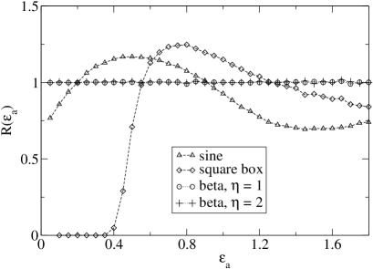
Figure 1: Ratio $R(\varepsilon_{a})$ of forward and backward probabilities of a transition path; $R(\varepsilon_{a})\neq 1$ indicates a breaking of detailed balance. Distributions $\psi(q)$ used are the sine-like distribution ($\vartriangle$) and the ‘square box’ one ($\diamond$) –see text for details. Results for beta $\psi(q)$ with $\eta=1$ ($\circ$) and $\eta=2$ ($+$) are also presented for comparison, showing as expected that detailed balance is satisfied for these distributions.

IV.2 Numerical renormalization procedure

Even though detailed balance is broken microscopically when $\psi(q)$ is different from a beta law, one can wonder whether the macroscopic properties of the model differ significantly or not from that in the presence of detailed balance. Indeed, some studies Grinstein ; Tauber have shown that a weak breaking of detailed balance does not influence the critical properties of particular classes of spin models. In the present model, numerical simulations suggest that even for distributions $\psi(q)$ with a behavior far from beta laws, no spatial correlations appear within two-points functions. Note that this result is also consistent with the vanishing of two-point correlations in the ‘q-model’ for granular matter Snoeijer , which presents some formal similarities (although in a different spirit), but also important differences, with the present model. In particular, the q-model is static, and the role played by time here corresponds to the vertical space direction. In addition, the dynamics of the q-model is equivalent to a synchronous dynamics, and the conserved quantity is linear since it represents the vertical component of forces between grains.

In order to test whether macroscopic properties are influenced or not by the breaking of detailed balance at the microscopic level, one can try to use a renormalization group approach. Even though such an approach might not seem natural in a context where no diverging length scale appears, this is actually a standard way to compute the effective dynamics at a coarse-grained level. Since no analytical solution is available for $\psi(q)$ different from a beta law, one has to resort to numerical simulations.

To this aim, the following renormalization procedure is introduced. The $d$-dimensional lattice is divided into cells (or blocks) of linear size $L$, and the effective dynamics between cells is measured from numerical simulations of the microscopic dynamics. To be more specific, when running the microscopic dynamics, one has to choose at random a link of the lattice at each time step, and to redistribute the energy over the link. If both sites of this link belong to the same block, then the redistribution is only an intra-block dynamics, and corresponds precisely to the degrees of freedom that have to be integrated out by the renormalization procedure. As a result, nothing is recorded during this particular process.

On the contrary, if the chosen link lies between two different cells, then the process is considered as a redistribution between blocks, and the effective fraction $q_{R}$ of energy redistributed is computed. Having chosen an orientation of the lattice, one can label for instance by $1$ and $2$ the two blocks involved in the process. Clearly, the total energy of these two blocks is conserved during this process. One thus computes the energy $E_{b}^{1}$ and $E_{b}^{2}$ of each block, and defines the effective fraction $q_{R}$ as the ratio:

$$q_{R}=\frac{E_{b}^{1}}{E_{b}^{1}+E_{b}^{2}}$$ (74)

To obtain the renormalized energy, one should actually divide $E_{b}$ by the size of the block (so that the energy density is conserved), but this is not essential here since we consider only energy ratios. The histogram of the values of $q_{R}$ obtained when running the microscopic dynamics is recorded, which gives the renormalized distribution $\psi_{L}(q)$. One would like to test if for large values of $L$, detailed balance is recovered, which would mean that the distribution $\psi_{L}(q)$ converges (in some sense to be specified) towards a beta law. As usual with renormalization procedures, the correct way to obtain large block sizes is not to consider large blocks from the beginning, but instead to start from small blocks and to iterate the procedure until the desired size is reached.

As a result, we started from cells of size $L=2$ and computed successively $\psi_{2}(q)$, $\psi_{4}(q)$, $\psi_{8}(q)$, etc., by applying recursively the same procedure with a microscopic dynamics defined by the renormalized $\psi_{L}(q)$ obtained at the step before. Numerical results obtained starting from an initial distribution $\psi(q)=\frac{\pi}{2}|\sin(2\pi q)|$ are shown on Fig. 2, for space dimensions $d=1$ and $d=2$. For $L\geq 4$, the resulting distributions $\psi_{L}(q)$ can be very well fitted by beta laws, i.e. by a test distribution $\psi_{\rm test}(q)$ of the form

$$\psi_{\rm test}(q)=\frac{\Gamma(2\eta_{L})}{\Gamma(\eta_{L})^{2}}\,[q(1-q)]^{\eta_{L}-1}$$ (75)

with only one free parameter $\eta_{L}$. This parameter $\eta_{L}$ is an increasing function of $L$, which can be easily understood from the fact that increasing the size of the blocks reduces the fluctuations of the energy from one block to another. So if one lets the size $L$ go to infinity, the distribution $\psi_{L}(q)$ eventually converges to a Dirac delta function centered on $q=\frac{1}{2}$. This means that the beta laws found from fitting the data are to be understood as pre-asymptotic distributions rather than as true limit distributions.

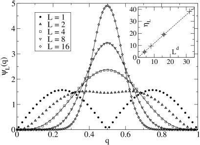
Figure 2: Renormalized distribution $\psi_{L}(q)$ for increasing sizes $L$, in dimension $d=1$. Full lines correspond to one-parameter fits with beta distributions. Inset: parameter $\eta_{L}$ from the fit plotted as a function of $L^{d}$ for $d=1$ ($+$) and $d=2$ ($\circ$); dashed line is the mean-field prediction given in Eq. (93).

Very interestingly, the fitting parameter $\eta_{L}$ is found to be linear with $L^{d}$, as seen in the inset of Fig. 2. This behavior can be interpreted in the following way, assuming that the initial distribution $\psi(q)$ is a beta law with parameter $\eta$. As seen from the calculations done in Sect. II.3, the local distribution of the energy $\varepsilon_{i}=g(x_{i})$ is given by a gamma law of exponent $\eta$ and scale parameter $\beta=1/T_{th}$:

$$p(\varepsilon_{i})=\frac{\beta^{\eta}}{\Gamma(\eta)}\,\varepsilon_{i}^{\eta-1}e^{-\beta\varepsilon_{i}}$$ (76)

The $\varepsilon_{i}$’s are independent random variables, so that the block energies $E_{b}$, defined as:

$$E_{b}=\sum_{i\in{\rm block}}\varepsilon_{i}$$ (77)

are distributed according to beta laws with exponent $\eta L^{d}$, where $L^{d}$ is the number of sites within a block. Then taking the ratio $q_{R}=E_{b}^{1}/(E_{b}^{1}+E_{b}^{2})$, one obtains for $q_{R}$ a beta distribution of parameter $\eta L^{d}$, as is well-known from the properties of gamma laws.

So starting from a beta law for $\psi(q)$, the above analytical argument shows that beta laws are again obtained from the renormalization procedure, with a parameter $\eta_{L}$ linear in $L^{d}$. Interestingly, the coefficient of proportionality is precisely the parameter $\eta$ of the microscopic law $\psi(q)$. So when starting from an arbitrary distribution $\psi(q)$, it is natural to define an effective parameter $\eta_{e}$ from the fitting parameter $\eta_{L}$ as:

$$\eta_{e}=\frac{\eta_{L}}{L^{d}}$$ (78)

One can then interpret $\eta_{e}$ as the parameter of the microscopic beta law which would give the same macroscopic behavior of the system as the initial distribution $\psi(q)$.

IV.3 Mean-field predictions

In this section, we aim to predict within a mean-field framework the effective exponent $\eta_{e}$ introduced above, for an arbitrary distribution $\psi(q)$. In a mean-field description, one assumes that the two-site steady-state distribution $P_{2}(x_{1},x_{2})$ can be factorized as a product of one-site distributions:

$$P_{2}(x_{1},x_{2})=P_{1}(x_{1})\,P_{1}(x_{2})$$ (79)

This assumption is valid if $\psi(q)$ is a beta law, as can be seen from Eq. (III.1.2). For more general $\psi(q)$, it remains a priori only an approximation. In order to deal with the renormalization procedure, it is more convenient to work with the distribution $p(\varepsilon_{i})$ of the local energy $\varepsilon_{i}\equiv g(x_{i})$, rather than with $P_{1}(x_{i})$. In terms of the variables $\{\varepsilon_{i}\}$, the redistribution rules read:

$$\varepsilon_{j}^{\prime}=q\,(\varepsilon_{j}+\varepsilon_{k}),\qquad\varepsilon_{k}^{\prime}=(1-q)\,(\varepsilon_{j}+\varepsilon_{k})$$ (80)

Numerical simulations show that after a sufficient coarse-graining by the renormalization procedure, the renormalized distribution $\psi_{L}(q)$ becomes a beta law with parameter $\eta_{L}=\eta_{e}\,L^{d}$. The associated renormalized distribution of the block energies $E_{b}$ is then a gamma law with exponent $\eta_{L}$ and scale parameter $\beta_{L}$:

$$p_{L}(E_{b})=\frac{\beta_{L}^{\eta_{L}}}{\Gamma(\eta_{L})}\,E_{b}^{\eta_{L}-1}e^{-\beta_{L}E_{b}}$$ (81)

The exponent $\eta_{L}$ can be determined from the first and second moments of the distribution $p_{L}(E_{b})$. Indeed, one finds an average value $\langle E_{b}\rangle=\eta_{L}/\beta_{L}$, and a variance ${\rm Var}(E_{b})=\eta_{L}/\beta_{L}^{2}$, with ${\rm Var}(E_{b})=\langle E_{b}^{2}\rangle-\langle E_{b}\rangle^{2}$. As a result, $\eta_{L}$ is given by:

$$\eta_{L}=\frac{\langle E_{b}\rangle^{2}}{\langle E_{b}^{2}\rangle-\langle E_{b}\rangle^{2}}$$ (82)

If the initial distribution $p(\varepsilon_{i})$ is factorized, the block energies $E_{b}$ are sums of independent random variables –see Eq. (77). So the average value and the variance of $E_{b}$ are simply the sums of the average and variance of the variables $\varepsilon_{i}$:

$$\langle E_{b}\rangle=\langle\varepsilon\rangle\,L^{d},\qquad{\rm Var}(E_{b})={\rm Var}(\varepsilon)\,L^{d}$$ (83)

From Eq. (82), the effective exponent $\eta_{e}=\eta_{L}/L^{d}$ is thus found to be:

$$\eta_{e}=\frac{\langle\varepsilon\rangle^{2}}{{\rm Var}(\varepsilon)}$$ (84)

So if we know the two first moments of the distribution $p(\varepsilon)$, we are able to compute $\eta_{e}$.

To obtain these moments for an arbitrary $\psi(q)$, we use the following steady-state master equation for the distribution $p(\varepsilon)$:

$$p(\varepsilon) = \int_{0}^{\infty}d\varepsilon_{1}\,p(\varepsilon_{1})\int_{0}^{\infty}d\varepsilon_{2}\,p(\varepsilon_{2})\times$$ (85)

$$\quad\int_{0}^{1}dq\,\psi(q)\,\delta\left(\varepsilon-q(\varepsilon_{1}+\varepsilon_{2})\right)$$

This equation can be considered as describing the redistribution process over an isolated single link. Yet, it can also be derived from a mean-field version of the model, in which redistributions can occur over any pair of sites of the system –see Appendix B.

Introducing the Laplace transform $\hat{p}(s)$ defined as

$$\hat{p}(s)\equiv\int_{0}^{\infty}d\varepsilon\,e^{-s\varepsilon}\,p(\varepsilon)$$ (86)

one can rewrite Eq. (85) as

$$\hat{p}(s)=\int_{0}^{1}dq\,\psi(q)\int_{0}^{\infty}d\varepsilon_{1}\,p(\varepsilon_{1})\int_{0}^{\infty}d\varepsilon_{2}\,p(\varepsilon_{2})\,e^{-sq(\varepsilon_{1}+\varepsilon_{2})}$$ (87)

The integrals over $\varepsilon_{1}$ and $\varepsilon_{2}$ can be factorized into a product of Laplace transforms:

$$\hat{p}(s)=\int_{0}^{1}dq\,\psi(q)\,\hat{p}(qs)^{2}$$ (88)

From the last equation, the successive moments of $p(\varepsilon)$ can be obtained, since they are given by the derivatives of $\hat{p}(s)$ in $s=0$:

$$\langle\varepsilon\rangle=-\frac{d\hat{p}}{ds}\Big{|}_{s=0},\qquad\langle\varepsilon^{2}\rangle=\frac{d^{2}\hat{p}}{ds^{2}}\Big{|}_{s=0}$$ (89)

Note also that by definition, $\hat{p}(0)=1$. Taking the first derivative of Eq. (88) in $s=0$, one recovers that $\langle q\rangle=\frac{1}{2}$. More interestingly, the second derivative of Eq. (88) yields:

$$\frac{d^{2}\hat{p}}{ds^{2}}\Big{|}_{s=0}=2\int_{0}^{1}dq\,q^{2}\,\psi(q)\left[\left(\frac{d\hat{p}}{ds}\Big{|}_{s=0}\right)^{2}+\frac{d^{2}\hat{p}}{ds^{2}}\Big{|}_{s=0}\right]$$ (90)

In terms of moments, the last equation reads:

$$\langle\varepsilon^{2}\rangle=2\langle q^{2}\rangle\left[\langle\varepsilon\rangle^{2}+\langle\varepsilon^{2}\rangle\right]$$ (91)

To compute $\eta_{e}$, we only need the ratio $\langle\varepsilon\rangle^{2}/\langle\varepsilon^{2}\rangle$, which is easily found from the preceding equation:

$$\frac{\langle\varepsilon^{2}\rangle}{\langle\varepsilon\rangle^{2}}=\frac{2\langle q^{2}\rangle}{1-2\langle q^{2}\rangle}$$ (92)

Taking into account that $\langle q\rangle=\frac{1}{2}$, $\eta_{e}$ is found to be:

$$\eta_{e}=\frac{1}{8{\rm Var}(q)}-\frac{1}{2}$$ (93)

IV.4 Analytical arguments

To conclude this section dedicated to renormalization group approaches, we wish to give a heuristic analytical argument that may help to understand the numerical results presented on Fig. 2. As explained above, the renormalization can be worked out exactly in the case where $\psi(q)$ is a beta law. The numerical procedure shows that other distributions $\psi(q)$ converge to beta laws under renormalization. From an analytical point of view, it is more convenient to work with the distribution $p(\varepsilon)$ of the local energy, rather than with $\psi(q)$. A beta $\psi(q)$ is associated to a gamma law for $p(\varepsilon)$ so that it would be interesting to check analytically whether an arbitrary $p(\varepsilon)$ converges to a gamma law under renormalization. Note that an implicit assumption here is that the $N$-site energy distribution is factorized, in a mean-field spirit.

A general calculation for an arbitrary initial distribution $p(\varepsilon)$ is in fact highly non trivial. We thus restrict the following calculations to an initial $p(\varepsilon)$ which differs only slightly from a gamma law:

$$p(\varepsilon)=p_{\gamma}(\varepsilon)+\lambda\delta p(\varepsilon)$$ (94)

where $\lambda\ll 1$ is an arbitrarily small parameter, and $p_{\gamma}(\varepsilon)$ is a gamma distribution similar to that used in Eq. (76). Since the renormalization conserves the average energy, $p(\varepsilon)$ and $p_{\gamma}(\varepsilon)$ must have the same average value $\overline{\varepsilon}$ so as to become equivalent after renormalization. Taking also into account the normalization condition, $\delta p(\varepsilon)$ has to satisfy

$$\int_{0}^{\infty}d\varepsilon\,\delta p(\varepsilon)=0,\qquad\int_{0}^{\infty}d\varepsilon\,\varepsilon\,\delta p(\varepsilon)=0.$$ (95)

Let $M\equiv L^{d}$ be the number of sites in a block. The renormalized energy $\varepsilon_{R}$ is given by

$$\varepsilon_{R}=\frac{1}{M}\sum_{i\in{\rm block}}\varepsilon_{i}$$ (96)

The distribution of $p_{1}(\varepsilon_{R})$ is more easily obtained using a Laplace transform:

$$\hat{p_{1}}(s)=\hat{p}(s/M)^{M}$$ (97)

Obviously, a fixed point for this equation is $p(s)=e^{-s\overline{\varepsilon}}$, which leads to $p(\varepsilon)=\delta(\varepsilon-\overline{\varepsilon})$. The aim of the present calculation is to see whether $p(\varepsilon)$ and $p_{\gamma}(\varepsilon)$ converge ‘in the same way’ or not toward the delta distribution.

Replacing Eq. (94) into Eq. (97) and expanding up to first order in $\lambda$, one has:

$$\delta\hat{p}_{1}(s)=M\,\hat{p}_{\gamma}\left(\frac{s}{M}\right)^{M-1}\delta\hat{p}\left(\frac{s}{M}\right)$$ (98)

Iterating $K$ times the renormalization procedure, one gets:

$$\delta\hat{p}_{K}(s)=M^{K}\,\delta\hat{p}\left(\frac{s}{M^{K}}\right)\prod_{n=0}^{K-1}\hat{p}_{\gamma,n}\left(\frac{s}{M^{K-n}}\right)^{M-1}$$ (99)

The renormalized gamma distribution $\hat{p}_{\gamma,n}(s)$ obtained after $n$ iterations is given by

$$\hat{p}_{\gamma,n}(s)=\left(1+\frac{s\overline{\varepsilon}}{\eta\,M^{n}}\right)^{-\eta M^{n}}$$ (100)

Then Eq. (99) can then be rewritten:

$$\delta\hat{p}_{K}(s)=M^{K}\,\left(1+\frac{s\overline{\varepsilon}}{\eta\,M^{K}}\right)^{-\eta(M^{K}-1)}\,\delta\hat{p}\left(\frac{s}{M^{K}}\right)$$ (101)

Using the relation

$$\lim_{K\to\infty}\left(1+\frac{s\overline{\varepsilon}}{\eta\,M^{K}}\right)^{-\eta(M^{K}-1)}=e^{-s\overline{\varepsilon}}$$ (102)

one ends up with

$$\delta\hat{p}_{K}(s)\approx M^{K}\,e^{-s\overline{\varepsilon}}\,\delta\hat{p}\left(\frac{s}{M^{K}}\right)$$ (103)

Expanding $\delta\hat{p}(s)$ in power of $s$ for $s\to 0$, one has

$$\delta\hat{p}(s)=g_{2}s^{2}+{\cal O}(s^{3})$$ (104)

since the terms of order $0$ and $1$ vanish due to Eq. (95). This yields:

$$\delta\hat{p}_{K}(s)\approx e^{-s\overline{\varepsilon}}\,\frac{g_{2}s^{2}}{M^{K}}$$ (105)

which goes to $0$ when $K\to\infty$ as expected. Yet, this is not enough to show that $p(\varepsilon)$ and $p_{\gamma}(\varepsilon)$ converge ‘in the same way’ toward the distribution $\delta(\varepsilon-\overline{\varepsilon})$. To do so, one has to show that $\delta\hat{p}_{K}(s)$ goes to $0$ more rapidly than the ‘distance’ between $\hat{p}_{\gamma,K}(s)$ and the infinite $K$ limit

$$\hat{p}_{\gamma,\infty}(s)=e^{-s\overline{\varepsilon}}$$ (106)

A way to quantify this ‘distance’ is to introduce the quantity:

$$D_{K}=\int_{0}^{\infty}ds\,\big{|}\hat{p}_{\gamma,K}(s)-\hat{p}_{\gamma,\infty}(s)\big{|}$$ (107)

which can be shown easily to take the asymptotic form:

$$D_{K}\approx\frac{1}{\eta\,\overline{\varepsilon}M^{K}}$$ (108)

The convergence criterion can be written as

$$\lim_{K\to\infty}\frac{\delta\hat{p}_{K}(s)}{D_{K}}=0$$ (109)

This requires that $g_{2}=0$ in the expansion of $\delta\hat{p}_{0}(s)$, which implies that the distributions $p(\varepsilon)$ and $p_{\gamma}(\varepsilon)$ have the same variance $\sigma^{2}=\sigma_{\gamma}^{2}$. Such a condition is actually natural, as the variance becomes $\sigma_{K}^{2}=\sigma^{2}/M^{K}$ under renormalization. If the two distributions take the same form after renormalization, they should have in particular the same variance $\sigma_{K}^{2}=\sigma_{\gamma,K}^{2}$, and one recovers $\sigma^{2}=\sigma_{\gamma}^{2}$.

Obviously, the above arguments are not fully rigorous, and remain somehow at a heuristic level, but they already give some insights on the mechanisms leading to the convergence process observed numerically.

V Conclusion

The class of models studied in the present paper is a very interesting example in which one can define a meaningful temperature $T_{th}$ from the conditional energy distribution of two subsystems, a procedure similar to the one used in the equilibrium microcanonical ensemble. These models exhibit a rich behavior which includes linear as well as non linear response to a perturbation, and linear or non linear fluctuation-dissipation relations when the response is linear. Our major result is that the temperature $T_{FD}$ deduced from the (linear) FDR does not coincide with the statistical temperature $T_{th}$, and that $T_{FD}$ does not take equal values in two subsystems when one considers an inhomogenous version of the model. This suggests that FDR are not necessarily the relevant way to define a temperature in the context of non glassy out-of-equilibrium steady-state systems.

In addition, a numerical renormalization procedure suggests that detailed balance is generically restored on a coarse-grained level when it is not satisfied by the microscopic dynamics. This renormalization procedure yields a new parameter $\eta_{e}$ describing the deviation from equilibrium, which can be analytically computed within a mean-field approximation. This leads to a macroscopic description of the system with two parameters, namely $T_{th}$ and $\eta_{e}$.

Finally, from a more general point of view, the present work raises important questions concerning the way to extend the concepts of statistical mechanics and thermodynamics to out-of-equilibrium systems. On the one hand, the very definition of thermometers in non-equilibrium systems appears to be a highly non trivial issue, as the way to couple the thermometer to the system is not unique. Thus one may need to impose some –still unknown– prescriptions on the coupling to get a well-defined measurement. On the other hand, the present work may be of some relevance for the description of non-equilibrium systems in which a global quantity is conserved. For instance, one may think of the two-dimensional turbulence where the vorticity is globally conserved Kraichnan ; Lesieur ; Frisch , or of dense granular matter in a container with fixed volume, in which the sum of the local free volumes would also be conserved. Indeed, the present model, for which the probability distribution is generically non uniform over the mutually accessible states (i.e. states with the same value of the energy, or volume, etc.) may allow in particular to go beyond the so-called Edwards’ hypotheses Edwards ; Mehta ; Barrat00 , according to which all accessible blocked states have the same probability to be occupied.

Acknowledgements

E.B. is particularly grateful to J.-P. Bouchaud and F. Lequeux for important contributions which were at the root of the present work. This work has been partially supported by the Swiss National Science Foundation.

Appendix A Time-dependent entropy

In this appendix, we show that the time-dependent entropy $S_{E}(t)$ defined in Eq. (36) is a non-decreasing function of time. Let us first recall its definition:

$$S_{E}(t)=-\int\prod_{i=1}^{N}dx_{i}\,P(\{x_{i}\},t)\,\ln\frac{P_{E}(\{x_{i}\},t)}{f(\{x_{i}\})}$$ (110)

with $f(\{x_{i}\})\equiv\prod_{i=1}^{N}|g^{\prime}(x_{i})|\,g(x_{i})^{\eta-1}$, and $P_{E}(\{x_{i}\},t)$ is the probability measure restricted to the hypersurface of given energy $E$:

$$P(\{x_{i}\},t)=P_{E}(\{x_{i}\},t)\;\delta\left(\sum_{i=1}^{N}g(x_{i})-E\right)$$ (111)

Taking the derivative with respect to time, one finds:

$$\frac{dS_{E}}{dt}=-\int\prod_{i=1}^{N}dx_{i}\,\frac{\partial P}{\partial t}(\{x_{i}\},t)\,\ln\frac{P_{E}(\{x_{i}\},t)}{f(\{x_{i}\})}$$ (112)

since the integral of the time derivative of the logarithm vanishes. One can then use the master equation to express $\partial P/\partial t$ as a function of $P(\{x_{i}\},t)$ and of the transition rates. The obtained expression can be symmetrized by permuting the integration variables $x_{i}$ and $x_{i}^{\prime}$ to get:

$$\frac{dS}{dt} = \frac{1}{2}\int\prod_{i=1}^{N}dx_{i}\,dx_{i}^{\prime}\,\left[W(\{x_{i}^{\prime}\}|\{x_{i}\})\,P(\{x_{i}\},t)-\right.$$ (113)

$$\qquad\qquad\qquad\left.W(\{x_{i}\}|\{x_{i}^{\prime}\})\,P(\{x_{i}^{\prime}\},t)\right]\,\times$$

$$\quad\qquad\left[\ln\frac{P_{E}(\{x_{i}\},t)}{f(\{x_{i}\})}-\ln\frac{P_{E}(\{x_{i}^{\prime}\},t)}{f(\{x_{i}^{\prime}\})}\right]$$

Now one can use the detailed balance relation Eq. (II.3):

$$W(\{x_{i}^{\prime}\}|\{x_{i}\})\,f(\{x_{i}\})=W(\{x_{i}\}|\{x_{i}^{\prime}\})\,f(\{x_{i}^{\prime}\})$$ (114)

and write $dS/dt$ in the following way:

$$\frac{dS}{dt} = \frac{1}{2}\int\prod_{i=1}^{N}dx_{i}\,dx_{i}^{\prime}\,W(\{x_{i}^{\prime}\}|\{x_{i}\})\,f(\{x_{i}\})\,\times$$ (115)

$$\quad\left[\frac{P_{E}(\{x_{i}\},t)}{f(\{x_{i}\})}-\frac{P_{E}(\{x_{i}^{\prime}\},t)}{f(\{x_{i}^{\prime}\})}\right]\,\times$$

$$\quad\left[\ln\frac{P_{E}(\{x_{i}\},t)}{f(\{x_{i}\})}-\ln\frac{P_{E}(\{x_{i}^{\prime}\},t)}{f(\{x_{i}^{\prime}\})}\right]$$

In this form, it is clear that the time derivative of the entropy is always positive. It vanishes only for the steady state distribution:

$$P_{E}(\{x_{i}\})=\frac{1}{Z_{N}(E)}\,f(\{x_{i}\})$$ (116)

and the corresponding maximum value of the entropy is equal to:

$$S(E)=\ln Z_{N}(E)$$ (117)

Appendix B Mean-field master equation

In section IV.3, a simple steady-state master equation was introduced to describe the one-site distribution $p(\varepsilon_{i})$ of the energy $\varepsilon_{i}\equiv g(x_{i})$ –see Eq. (85)– in the case of an arbitrary distribution $\psi(q)$. We show here how this simple equation can be derived from the master equation associated to a $N$-site model with infinite range interactions. Introducing such long range interactions is a usual way to build a mean-field version of a model. To be more specific, we generalize the model introduced in Eq. (4) in order to allow redistributions over any pair of sites $(j,k)$, and not only on the links of the lattice. As a result, the lattice becomes useless in this version of the model.

The transition rates read:

$$W(\{\varepsilon_{i}^{\prime}\}|\{\varepsilon_{i}\})=\frac{1}{N}\sum_{j<k}\left[\prod_{i\neq j,k}\delta(\varepsilon_{i}^{\prime}-\varepsilon_{i})\right]\times$$ (118)

$$\quad\delta(\varepsilon_{j}^{\prime}+\varepsilon_{k}^{\prime}-\varepsilon_{j}-\varepsilon_{k})\int_{0}^{1}dq\,\psi(q)\,\delta\left(\varepsilon_{j}^{\prime}-q(\varepsilon_{j}+\varepsilon_{k})\right)$$

where the sum runs over all pairs $(j,k)$. The factor $1/N$ is introduced so that each site keeps, in the thermodynamic limit $N\to\infty$, a probability per unit time of the order of one to be involved in a redistribution.

The stationary distribution $P_{MF}(\{\varepsilon_{i}\})$ satisfies the following master equation:

$$P_{MF}(\{\varepsilon_{i}\})\int\prod_{i=1}^{N}d\varepsilon_{i}^{\prime}\,W(\{\varepsilon_{i}^{\prime}\}|\{\varepsilon_{i}\})=$$ (119)

$$\quad\int\prod_{i=1}^{N}d\varepsilon_{i}^{\prime}\,W(\{\varepsilon_{i}\}|\{\varepsilon_{i}^{\prime}\})\,P_{MF}(\{\varepsilon_{i}^{\prime}\})$$

The first integral is the total exit rate from configuration $\{\varepsilon_{i}\}$, and is equal to $(N-1)/2$ from Eq. (118). So the last equation can be rewritten in a more explicit form:

$$P_{MF}(\{\varepsilon_{i}\})=\frac{2}{N(N-1)}\times$$

$$\quad\sum_{j<k}\int_{0}^{\infty}d\varepsilon_{j}^{\prime}\int_{0}^{\infty}d\varepsilon_{k}^{\prime}\,\delta(\varepsilon_{j}^{\prime}+\varepsilon_{k}^{\prime}-\varepsilon_{j}-\varepsilon_{k})\times$$ (120)

$$\quad\int_{0}^{1}dq\,\psi(q)\,\delta\left(\varepsilon_{j}-q(\varepsilon_{j}^{\prime}+\varepsilon_{k}^{\prime})\right)P_{MF}(\varepsilon_{j}^{\prime},\varepsilon_{k}^{\prime},\{\varepsilon_{i}\}_{i\neq j,k})$$

In order to go further, one has to assume that the distribution $P_{MF}(\{\varepsilon_{i}\})$ factorizes:

$$P_{MF}(\{\varepsilon_{i}\})=\prod_{i=1}^{N}p(\varepsilon_{i})$$ (121)

where $p(\varepsilon)$ is the one-site distribution. This assumption is justified in the limit of large $N$. Integrating over all variables except $\varepsilon_{1}$, one gets:

$$p(\varepsilon_{1})=\sum_{j=1}^{N-1}\sum_{k=j+1}^{N}\frac{2}{N(N-1)}\times$$ (122)

$$\int\prod_{i=2}^{N}d\varepsilon_{i}\,\prod_{i\neq j,k}p(\varepsilon_{i})\int_{0}^{\infty}d\varepsilon_{j}^{\prime}\,p(\varepsilon_{j}^{\prime})\int_{0}^{\infty}d\varepsilon_{k}^{\prime}\,p(\varepsilon_{k}^{\prime})\times$$

$$\delta(\varepsilon_{j}^{\prime}+\varepsilon_{k}^{\prime}-\varepsilon_{j}-\varepsilon_{k})\int_{0}^{1}dq\,\psi(q)\,\delta\left(\varepsilon_{j}-q(\varepsilon_{j}^{\prime}+\varepsilon_{k}^{\prime})\right)$$

The r.h.s. can then be decomposed into two terms, one corresponding to $i=1$ and the other one to $i>1$, which are called respectively $R_{1}$ and $R_{2}$ in the following:

$$p(\varepsilon_{1})=R_{1}+R_{2}$$ (123)

The first term $R_{1}$ is associated with redistributions involving site $j=1$ as well as another arbitrary site $k$. It is actually independent of $k$, so that $R_{1}$ is the sum of $(N-1)$ identical terms. Integrating over $\varepsilon_{k}$ removes the delta distribution $\delta(\varepsilon_{1}^{\prime}+\varepsilon_{k}^{\prime}-\varepsilon_{1}-\varepsilon_{k})$, and one finds:

$$R_{1} = \frac{2}{N}\int_{0}^{\infty}d\varepsilon_{1}^{\prime}\,p(\varepsilon_{1}^{\prime})\int_{0}^{\infty}d\varepsilon_{2}^{\prime}\,p(\varepsilon_{2}^{\prime})\times$$

$$\qquad\qquad\int_{0}^{1}dq\,\psi(q)\,\delta\left(\varepsilon_{1}-q(\varepsilon_{1}^{\prime}+\varepsilon_{2}^{\prime})\right)$$

On the other hand, the second term $R_{2}$ is the contribution from all the redistributions involving sites $j=2\ldots N$, but not site $j=1$. There are $(N-1)(N-2)/2$ such pairs of links, which all give the same contribution to $R_{2}$. So $R_{2}$ can be written:

$$R_{2} = \frac{N-2}{N}\,p(\varepsilon_{1})\,\int_{0}^{\infty}d\varepsilon_{2}^{\prime}\,p(\varepsilon_{2}^{\prime})\int_{0}^{\infty}d\varepsilon_{3}^{\prime}\,p(\varepsilon_{3}^{\prime})\times$$

$$\qquad\qquad\int_{0}^{1}dq\,\psi(q)\int_{0}^{\infty}d\varepsilon_{2}\,\delta\left(\varepsilon_{2}-q(\varepsilon_{2}^{\prime}+\varepsilon_{3}^{\prime})\right)$$

All the integrals in the r.h.s. of the above equation give a contribution equal to unity, so that $R_{2}$ reduces to:

$$R_{2}=\left(1-\frac{2}{N}\right)p(\varepsilon_{1})$$ (126)

Replacing the above results into Eq. (123), one finally obtains the following equation:

$$p(\varepsilon) = \int_{0}^{\infty}d\varepsilon_{1}\,p(\varepsilon_{1})\int_{0}^{\infty}d\varepsilon_{2}\,p(\varepsilon_{2})\times$$

$$\quad\int_{0}^{1}dq\,\psi(q)\,\delta\left(\varepsilon-q(\varepsilon_{1}+\varepsilon_{2})\right)$$

which is precisely Eq. (85).

References

- (1) For a review, see J. Casas-Vázquez and D. Jou, Rep. Prog. Phys. 66, 1937 (2003).
- (2) A. Q. Tool, J. Am. Ceram. Soc. 29, 240 (1946).
- (3) O. S. Narayanaswamy, J. Am. Ceram. Soc. 54, 491 (1971).
- (4) C. T. Moynihan et al., J. Am. Ceram. Soc. 59, 12 (1976).
- (5) L. F. Cugliandolo, J. Kurchan, and L. Peliti, Phys. Rev. E 55, 3898 (1997).
- (6) L. F. Cugliandolo and J. Kurchan, Phys. Rev. Lett. 71, 173 (1993).
- (7) G. Parisi, Phys. Rev. Lett. 79, 3660 (1997).
- (8) J.-L. Barrat and W. Kob, Europhys. Lett. 46, 637 (1999).
- (9) A. Barrat, J. Kurchan, V. Loreto, and M. Sellitto, Phys. Rev. Lett. 85, 5034 (2000); Phys. Rev. E 63, 051301 (2001).
- (10) F. Sciortino and P. Tartaglia, Phys. Rev. Lett. 86, 107 (2001).
- (11) L. Berthier and J.-L. Barrat, Phys. Rev. Lett. 89, 095702 (2002); J. Chem. Phys. 116, 6228 (2002).
- (12) F. Zamponi, G. Ruocco, and L. Angelani, e-print cond-mat/0403579.
- (13) For a review, see A. Crisanti and F. Ritort, J. Phys. A: Math. Gen. 36, R181 (2003).
- (14) T. S. Grigera and N. E. Israeloff, Phys. Rev. Lett. 83, 5038 (1999).
- (15) L. Bellon, S. Ciliberto, and C. Laroche, Europhys. Lett. 53, 511 (2001).
- (16) D. Hérisson and M. Ocio, Phys. Rev. Lett. 88, 257202 (2002); e-print cond-mat/0403112.
- (17) G. D’Anna, P. Mayor, A. Barrat, V. Loreto, and F. Nori, Nature 424, 909 (2003).
- (18) B. Abou and F. Gallet, e-print cond-mat/0403561.
- (19) G. Grinstein, C. Jayaprakash, and Y. He, Phys. Rev. Lett. 55, 2527 (1985).
- (20) U. C. Taüber, V. K. Akkineni, and J. E. Santos, Phys. Rev. Lett. 88, 045702 (2002).
- (21) A. Puglisi, A. Baldassarri, and V. Loreto, Phys. Rev. E 66, 061305 (2002).
- (22) A. Barrat, V. Loreto, and A. Puglisi, Physica A 334, 513 (2004).
- (23) F. Sastre, I. Dornic, and H. Chaté, Phys. Rev. Lett. 91, 267205 (2003).
- (24) B. N. Miller and P. M. Larson, Phys. Rev. A 20, 1717 (1979).
- (25) E. T. Jaynes, Phys. Rev. 106, 620 (1957).
- (26) E. Bertin, O. Dauchot, and M. Droz, Phys. Rev. Lett. 93, 230601 (2004).
- (27) E. Bertin, J.-P. Bouchaud, and F. Lequeux, to be published.
- (28) L. Berthier and J.-L. Barrat, Phys. Rev. Lett. 89, 095702 (2002).
- (29) P. K. Haff, J. Fluid. Mech. 134, 401 (1983).
- (30) B. Derrida, M. R. Evans, V. Hakim, and V. Pasquier, J. Phys. A: Math. Gen. 26, 1493 (1993).
- (31) S. Sandow, Phys. Rev. E 50, 2660 (1994).
- (32) J. H. Snoeijer and J. M. J. van Leeuwen, Phys. Rev. E 65, 051306 (2002).
- (33) R. H. Kraichnan and D. Montgomery, Rep. Prog. Phys. 43, 547 (1980).
- (34) M. Lesieur, Turbulence in Fluids, 2nd edition, Kluwer, Dordrecht (1990).
- (35) U. Frisch, Turbulence, Cambridge University Press, Cambridge (1995).
- (36) S. F. Edwards, in Granular Matter: An Interdisciplinary Approach, edited by A. Mehta (Springer-Verlag, New-York, 1994), and references therein.
- (37) A. Mehta, R. J. Needs, and S. Dattagupta, J. Stat. Phys. 68, 1131 (1992).