Measuring the Kondo effect in the Aharonov-Bohm interferometer

Abstract

The conductance ${\cal G}$ of an Aharonov-Bohm interferometer (ABI), with a strongly correlated quantum dot on one arm, is expressed in terms of the dot Green function, $G_{dd}$, the magnetic flux $\phi$ and the non-interacting parameters of the ABI. We show that one can extract $G_{dd}$ from the observed oscillations of ${\cal G}$ with $\phi$, for both closed and open ABI’s. In the latter case, the phase shift $\beta$ deduced from ${\cal G}\approx A+B\cos(\phi+\beta)$ depends strongly on the ABI’s parameters, and usually $\beta\neq\pi/2$. These parameters may also reduce the Kondo temperature, eliminating the Kondo behavior.
PACS numbers: 73.21.-b, 73.23.-b, 71.27.+a, 72.10.Fk

The recent observation of the Kondo effect in quantum dots (QD’s), whose parameters can be tuned continuously [1], has been followed by much theoretical and experimental activity. For temperatures $T$ below the Kondo temperature $T_{K}$, the spin of an electron localized on the QD is dynamically screened by the electrons in the Fermi sea, yielding a large conductance ${\cal G}$ through the QD, close to the unitary value $2e^{2}/h$, and a transmission phase $\alpha$ equal to $\pi/2$ [2, 3]. A good tool to test these predictions involves embedding the strongly-correlated QD on one arm of an Aharonov-Bohm interferometer (ABI). Indeed, such experiments were carried out for both a closed (two-terminal) ABI [4] and an open (multi-terminal) ABI [5]. Both experiments exhibited the Aharonov-Bohm oscillations with the normalized flux $\phi=e\Phi/\hbar c$. The former experiments exhibited the expected “phase rigidity”, with ${\cal G}$ an even function of $\phi$ [6]. However, there has been no quantitative analysis of these data. The latter experiments attempted to measure the transmission phase, and found a variety of behaviors which were inconsistent with the expected value of $\pi/2$. As a result, Ji et al. [5] stated that “the full explanation of the Kondo effect may go beyond the framework of the Anderson model”. Theoretical attempts to discuss related issues have concentrated on the dot alone (when it is detached from the ABI) [3, 7], or applied various techniques [8, 9, 10] to the QD on simple models of the closed ABI. However, it has not been very clear how to make quantitative comparisons of theory and experiment.

Most of the theoretical discussions of QD’s concentrate on the retarded Green function for electrons with energy $\omega$ on the QD, $G_{dd}(\omega)$ (we ignore the spin index, since we assume no magnetic asymmetry). For a simple QD, connected to a broad electronic band, the $T=0$ transmission amplitude for electrons going through the QD is proportional to $G_{dd}(\epsilon_{F})$, where $\epsilon_{F}$ is the Fermi energy (taken as zero below) [2, 11]. However, measuring the conductance only yields $|G_{dd}(0)|^{2}$, with no information on the phase. The ABI experiments were thus intended to measure both the magnitude and the phase of $G_{dd}$, and compare with theory. In this paper we concentrate on the following question: given experimental data on the flux dependent conductance of the ABI, ${\cal G}(\phi)$, how can we deduce the “intrinsic” Green function $G_{dd}$? An earlier paper [12] answered this question for non-interacting electrons on a simple model for a closed ABI, and made some speculations on the interacting case. Another paper [13] showed that for non-interacting electrons, the phase shift measured in the open ABI depends on details of the opening. Here we show that for strongly correlated electrons, ${\cal G}(\phi)$ is much more sensitive to the specific details of the ABI’s. We give explicit instructions for extracting $G_{dd}$ from the measured ${\cal G}(\phi)$, and show that the opening has much stronger effects in the Kondo regime, possibly explaining the puzzling experiments [5].

Our qualitative results should apply for a large class of ABI’s. For simplicity, we demonstrate them for the specific Anderson model shown in Fig. 1, which captures the important ingredients. The conductance ${\cal G}$ is measured between the two leads which are attached to sites “L” and “R” on the ABI ring. The QD (denoted “D”) is connected to L (R) via $n_{l}$ ($n_{r}$) sites. The lower “reference” branch contains $n_{0}$ sites. Except for the QD, we use a tight binding model, with the real hopping matrix elements as indicated in the figure. Site energies are $\epsilon_{l},~{}\epsilon_{r}$ and $\epsilon_{0}$ on the respective branches, $\epsilon_{L},~{}\epsilon_{R}$ on sites L and R and zero on the leads. Using gauge invariance, we introduce the normalized flux $\phi$ as a phase factor in $J_{D1}=J_{1D}^{\ast}=j_{l}e^{i\phi}$. The Hamiltonian on the dot is ${\cal H}_{d}=\epsilon_{d}\sum_{\sigma}n_{d\sigma}+Un_{d\uparrow}n_{d\downarrow}$, with obvious notations. Here we assume that the transport is dominated by the level $\epsilon_{d}$ on the QD. We also assume that $U$ is very large, and ignore the resonance at $2\epsilon_{d}+U$. Figure 1 generalizes earlier models [8, 9], by adding the internal structure on the links between D, L and R. Some such structure always exists in experiments, and may have important effects on the observed conductance (see below). For the open ABI, each dashed line represents an additional lead, with a hopping matrix element $-J_{X}$ on its first bond [13].

FIG. 1.: The model for the ABI, with $n_{l}=n_{r}=3,~{}n_{0}=5$.

For $T\ll T_{K}$, it is sufficient to calculate ${\cal G}$ at $T=0$. Irrespective of the above details, one has

$${\cal G}=\frac{2e^{2}}{h}4\Gamma_{L}(0)\Gamma_{R}(0)\big{|}G_{LR}(\omega=0)\big{|}^{2},$$ (1)

where $G_{LR}(\omega)$ is the Fourier transform of the retarded Green function involving a creation of an electron at site R and an annihilation of an electron at site L at time $t$ later [14]. Also, $\Gamma_{L,R}(\omega)=-\Im\Sigma^{0}_{L,R}(\omega)$, where $\Sigma^{0}_{L,R}$ is the self-energy generated at sites L or R due to the leads. Since interactions exist only on the dot, one can use the equations of motion to express all the retarded Green functions $G_{\alpha\beta}$ in terms of $G_{dd}$. If $g_{\alpha\beta}$ denotes the Green functions of the whole network without the QD and the two bonds connected to it, then it is straightforward to obtain [15] the relation

$$G_{LR}=g_{LR}+\sum_{\alpha\beta}g_{L\alpha}J_{\alpha D}J_{D\beta}g_{\beta R}G_{dd},$$ (2)

where in our model the only non-zero $J_{\alpha\beta}$’s are $J_{D1}=J_{1D}^{\ast}=j_{l}e^{i\phi}$ and $J_{DR}=J_{RD}=j_{r}$ (see Fig. 1).

For the non-interacting case, one has

$$G_{dd}=1/[\omega-\epsilon_{d}-\Sigma_{0}(\omega)],$$ (3)

with the non-interacting self-energy

$$\Sigma_{0}(\omega)=\sum_{\alpha\beta}J_{D\alpha}g_{\alpha\beta}(\omega)J_{\beta D}\equiv\delta\epsilon_{d}(\omega)-i\Delta_{0}(\omega).$$ (4)

Since the phase $\phi$ is only contained in $J_{D1}=J_{1D}^{\ast}$, the complex matrix $g_{\alpha\beta}$ is independent of $\phi$ and obeys $g_{\alpha\beta}=g_{\beta\alpha}$. Therefore,

$$\Sigma_{0}(\omega)=j_{l}^{2}g_{11}+j_{r}^{2}g_{NN}+2j_{l}j_{r}g_{1N}\cos\phi$$ (5)

is an even function of $\phi$. Except for the very special case $n_{l}=n_{r}=n_{0}=0$ (discussed e.g. in Refs. [8, 9]), $g_{1N}$ is not a real number, and therefore both $\delta\epsilon_{d}(\omega)$ and $\Delta_{0}(\omega)$ oscillate with $\phi$,

$$\delta\epsilon_{d}=a_{1}+b_{1}\cos\phi;\ \ \Delta_{0}=a_{2}+b_{2}\cos\phi.$$ (6)

Using these expressions, Eq. (2) can be written as

$$G_{LR}=g_{LR}G_{dd}\Bigl{(}[G_{dd}]^{-1}+\Sigma_{0}+\sum_{\alpha\beta}J_{D\alpha}w_{\alpha\beta}J_{\beta D}\Bigr{)},$$ (7)

with $w_{\alpha\beta}\equiv g_{\alpha R}g_{L\beta}/g_{LR}-g_{\alpha\beta}$. In calculating the necessary $g_{\alpha\beta}$’s, it is convenient to first eliminate all the leads, replacing them by site self-energies. For example, at site L we replace the bare Green function $1/(\omega-\epsilon_{L})$ by $1/[\omega-\epsilon_{L}-\Sigma^{0}_{L}(\omega)]$. For our one-dimensional leads one has $\Sigma^{0}_{L}(\omega)=-e^{i|q|a}J_{L}^{2}/J$, where $\omega=-2J\cos(qa)$ is the energy of the electron in the band of the leads (we assume all the leads to have the same $J$ and the same lattice constant $a$) [15]. The results remain valid also for more complex leads, as long as one uses the appropriate band-generated self-energies. For the remaining $N=n_{l}+n_{r}+n_{0}+2$ sites of the ring (without the QD), $g_{\alpha\beta}$ is then the inverse of a tri-diagonal $N\times N$ matrix, ${\cal M}_{\alpha\beta}=J_{\alpha\beta}+[\omega-\epsilon_{\alpha}-\Sigma^{0}_{\alpha}(\omega)]\delta_{\alpha\beta}$. For such a matrix, it turns out that one always has $w_{1N}=0$. Thus,

$${\cal G}={\cal G}_{ref}|G_{dd}|^{2}\big{|}G_{dd}^{-1}+\Sigma_{0}+x+ye^{-i\phi}\big{|}^{2},$$ (8)

where $x=j_{l}^{2}w_{11}+j_{r}^{2}w_{NN}$, $y=j_{l}j_{r}w_{N1}$ and the “reference” conductance ${\cal G}_{ref}\equiv(2e^{2}/h)4\Gamma_{L}(0)\Gamma_{R}(0)|g_{LR}|^{2}$ depend only on the parameters of the non-interacting parts of the ABI, and not on the QD parameters $\epsilon_{d}$ and $U$.

At $T=0$ the electrons must obey the Fermi liquid relations [16]. Specifically, at the Fermi energy one expects

$$\Im[G_{dd}^{-1}](\omega=0)\equiv\Delta_{0}(\omega=0).$$ (9)

This condition should hold for any network in which the QD is embedded, and is therefore true for both the closed and the open ABI. In the limit of a very large negative $\epsilon_{d}$, when $\langle n_{d}\rangle\rightarrow 1$, one also expects that $\Re[G_{dd}^{-1}](\omega=0)\rightarrow 0$. For the simple QD with two leads, one has $\Sigma_{0}(\omega)=\Sigma^{0}_{L}(\omega)+\Sigma^{0}_{R}(\omega)$, and in the symmetric case $\Gamma_{L}=\Gamma_{R}=\Delta_{0}/2$ the conductance reaches its unitary limit $2e^{2}/h$ [Eq. (1), with $G_{LR}\rightarrow G_{dd}$]. In this limit the phase of $G_{dd}$ becomes $\pi/2$ [2].

We now discuss the closed ABI. In this case, $w_{11},~{}w_{NN}$ and $w_{N1}$ and therefore also $x$ and $y$ are all real numbers. Using the Fermi liquid result (9) and Eq. (6), Eq. (8) becomes

$$\frac{{\cal G}_{closed}}{{\cal G}_{ref}}\equiv{\cal F}(\phi)\equiv\frac{(\zeta+r_{a}+r_{b}\cos\phi)^{2}+r_{y}^{2}\sin^{2}\phi}{\zeta^{2}+(1+r_{d}\cos\phi)^{2}},$$ (10)

with the dimensionless function $\zeta(\phi)=\Re[G_{dd}^{-1}]/a_{2}$ and constants $r_{a}=(a_{1}+x)/a_{2},~{}r_{b}=(b_{1}+y)/a_{2},~{}r_{y}=y/a_{2}$ and $r_{d}=b_{2}/a_{2}$. For the non-interacting case, $\zeta=[-\epsilon_{d}-\delta\epsilon_{d}(0)]/a_{2}$, and Eq. (10) generalizes the results of Ref. [12]. An example is shown on the LHS of Fig. 2. In the strongly correlated case and in the unitary limit, $\zeta=0$ and ${\cal G}_{closed}\rightarrow{\cal G}_{ref}{\cal F}_{0}(\phi)$. All the features in the $\phi$-dependence of ${\cal F}_{0}$ arise only due to the non-interacting parts of the ABI. Usually, Eq. (10) contains many harmonics. Except in special cases [8], it is not dominated by the second harmonic, and the period of ${\cal F}_{0}(\phi)$ is not simply doubled. An example of this dependence is seen (for large negative $\epsilon_{d}$) on the RHS of Fig. 2: except for the minima at $\phi=0$ and $\pi$, the maxima are not at $\pi/2$. Experimentally, one knows that one has reached this limit once the function ${\cal G}_{closed}(\phi)$ no longer changes with the gate voltage which governs $\epsilon_{d}$. The reference conductance ${\cal G}_{ref}$ can be measured by disconnecting the QD, i.e. setting $j_{l}=j_{r}=0$. Alternatively, ${\cal G}_{ref}$ can be absorbed in the scales of the parameters in the numerator of Eq. (10). Having determined ${\cal G}_{ref}$, one can determine the four real parameters $r_{a},~{}r_{b},~{}r_{y}$ and $r_{d}$ by a fit to ${\cal F}_{0}(\phi)$ (In practice, one only needs four values of the function) [17]. Having found these parameters, one can now move away from the unitary limit, and measure ${\cal G}_{closed}={\cal G}_{ref}{\cal F}(\phi)$. The unknown function $\zeta(\phi)$ can now be found from the quadratic equation

$$\zeta^{2}-2\zeta\frac{r_{a}+r_{b}\cos\phi}{{\cal F}-1}+\frac{{\cal F}-{\cal F}_{0}}{{\cal F}-1}(1+r_{d}\cos\phi)^{2}=0.$$ (11)

The solution should be chosen so that it decreases to zero at large negative $\epsilon_{d}$ and increases linearly with large positive $\epsilon_{d}$. Having found the solution, the phase $\alpha$ of $G_{dd}$ is then defined via

$$\cot\alpha=-\frac{\Re[G_{dd}^{-1}](\omega=0)}{\Delta_{0}(\omega=0)}\equiv-\frac{\zeta}{1+r_{d}\cos\phi}.$$ (12)

This phase, or equivalently $\Re[G_{dd}^{-1}]$, are the quantities obtained from theories.

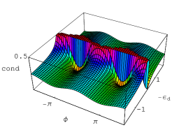
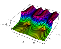
FIG. 2.: Conductance (in units of $2e^{2}/h$) through the closed ABI versus the normalized flux $\phi$ and the energy of the state on the dot $\epsilon_{d}$ (the gate voltage), without (LHS) and with interactions (RHS). $n_{l}=n_{r}=2,~{}n_{0}=3$, $J_{L}=J_{R}=J_{D}=1$, $j_{l}=j_{r}=.2,~{}i_{l}=i_{r}=.4$, $\epsilon_{l}=\epsilon_{r}=\epsilon_{0}=-.3,~{}\epsilon_{L}=\epsilon_{R}=0$. All energies are in units of $J$.

For demonstrating the qualitative dependence of ${\cal G}$ on $\phi$ and on the other parameters, we have used an approximate analytic solution of the equations of motion, truncated via decoupling of higher order Green functions [15]. In the limits $T=\omega=0$ and $U\rightarrow\infty$, this solution assumes the simple analytic form

$$\cot\alpha=-\frac{z\delta n-\frac{3}{4}\Bigl{(}z+\sqrt{z^{2}+\delta n(\frac{3}{2}-\delta n)}\Bigr{)}}{2\Bigl{[}\frac{3}{4}\delta n+z\Bigl{(}z+\sqrt{z^{2}+\delta n(\frac{3}{2}-\delta n)}\Bigr{)}\Bigr{]}},$$ (13)

where $z$ represents the value at $\omega=0$ of the non-interacting ratio

$$z(\omega)=[\omega-\epsilon_{d}-\delta\epsilon_{d}(\omega)]/[2\Delta_{0}(\omega)],$$ (14)

while $\delta n$ is related to the electron occupation on the dot via $\langle n_{d}\rangle=2(1-\delta n)$ (which should be determined self-consistently). In practice, $\delta n$ varies smoothly between $1/2$ (at $z\gg 1$) and 1 (at $z\ll-1$), and the results of calculations are not very sensitive to the details of this variation. Equation (13) interpolates between $\beta=\pi/2$ at $z\rightarrow\infty$ and $\beta=\pi$ for $z\rightarrow-\infty$. In the latter limit, $G_{dd}$ approaches the non-interacting form (3). Using Eq. (13) in Eq. (10) for a specific set of parameters yields the RHS of Fig. 2. One clearly sees the transition from the non-interacting behavior at large positive $\epsilon_{d}$ (compare with the LHS) to the unitary limit at large negative $\epsilon_{d}$. For different sets of parameters one reproduces qualitatively all the earlier results, including the Fano-Kondo effect [8]. We have used these results to imitate real experimental “data”, and were able to use the above algorithm to extract $\cot\alpha$ as in Eq. (12).

Note that the above analysis yields $G_{dd}$ for the QD on the ABI, where this function (and thus also the phase $\alpha$) depends explicitly on the flux $\phi$, via $z$. At $T=\omega=0$, we expect $\alpha$ to depend only on the ratio $z$ also for other theories. In our case, $z$ can be extracted from the experimental data via

$$z=-[\tilde{\epsilon}_{d}+r_{a}+(r_{b}-r_{y})\cos\phi]/(1+r_{d}\cos\phi),$$ (15)

where $\tilde{\epsilon}_{d}=(\epsilon_{d}-x)/a_{2}$ is just a shifted rescaled gate voltage. Having deduced the dependence of both $z$ and $\alpha$ on $\phi$, a parametric plot can yield $\alpha$ versus $z$, for comparison with single dot calculations. Alternatively, one can experimentally study the results as function of the coupling to the reference branch, $i_{l}$ and $i_{r}$. Extrapolation to $i_{l},~{}i_{r}\rightarrow 0$ would give the dependence of $\alpha$ on $\Sigma_{0}(0)$ for the upper branch alone. However, $\Sigma_{0}(\omega)$ still depends on the finite chains connecting D with L and R [18].

We now turn to the open ABI, with $J_{X}\neq 0$. Equation (8) remains correct, but now $x$ and $y$ become complex. Interestingly, Eq. (5) still holds, and $\Sigma_{0}$ is still an even function of $\phi$. In the unitary limit, ${\cal G}(\phi)$ has the exact form

$${\cal G}_{open}\rightarrow{\cal G}_{ref}\frac{A+B\cos(\phi+\tilde{\beta})+C\cos(2\phi+\gamma)}{(1+r_{d}\cos\phi)^{2}},$$ (16)

and we need six parameters to fit it. Note that all the ABI parameters (including ${\cal G}_{ref}$) now also depend on $J_{X}$. The two lower curves in the left panel of Fig. 3 show results in this limit. Note that the graphs are not sinusoidal, mainly due to the second term in the numerator and to the denominator in Eq. (16). Since one remains close to the Kondo resonance, the denominator continues to be important, modifying the 2-slit-like numerator. The asymmetric shape of each oscillation seems similar to that reported in Ref. [5]. The other curves in the same panel were derived using Eq. (13). Again, one observes the crossover to the non-interacting sinusoidal shape at large positive $\epsilon_{d}$. To extract a “transmission phase” from these curves, one can e.g. follow the maxima as function of $\epsilon_{d}$, or enforce a fit to the two-slit formula ${\cal G}_{open}\approx A+B\cos(\phi+\beta)$. Since now there is no well-defined zero to $\phi$, one can only deduce the relative change in the phase $\beta$. Setting $\beta=0$ at $\epsilon_{d}\rightarrow-\infty$, the RHS of Fig. 3 shows this relative phase versus $\epsilon_{d}$. For the parameters we used, the total change is about $0.8\pi$, far away from the expected change in $\alpha$, equal to $\pi/2$. The actual values depend on details of the ABI. This may explain the non-trivial values of the phases observed in Ref. [5]: they result from the experimental setup, and not from a breakdown of the Anderson theory.

FIG. 3.: LHS: Conductance through the open ABI versus $\phi$, at $\epsilon_{d}=(-1.5,~{}-1,~{}-.5,~{}0,~{}.5,~{}1,~{}1.5)J$, with interactions. Graphs are shifted up with increasing $\epsilon_{d}$. Parameters are the same as in Fig. 2, but with $J_{X}=.5$. RHS: The “measured” phase shift $\beta$ (in units of $\pi$) versus $\epsilon_{d}$.

Finally, a few words about non-zero $T$ or $\omega$. Generally, $T$ and $\omega$ enter into $G_{dd}$ similarly. In the approximate solution of Ref. [15], one ends up with a competition between the variable $z(\omega)$ of Eq. (14) and $\log(D/T)$ or $\log(D/\omega)$, where $2D=4J$ is the width of the band in the leads. This competition yields estimates of $T_{K}$,

$$\log(T_{K}/D)=\pi[\epsilon_{d}+\delta\epsilon_{d}(0)]/\Delta_{0}(0).$$ (17)

Although more accurate theories end up with different expressions, all of them end up with a strong dependence on the ratio which appears on the RHS. In our case, this ratio oscillates strongly with $\phi$, opening the possibility that for different fluxes the QD is below or above $T_{K}$. We emphasize the appearance of $\delta\epsilon_{d}$ in the numerator, ignored in some papers.

At non-zero $T$, the “intrinsic” phase of the QD is expected to start at 0 for large negative $\epsilon_{d}$ [where $T>T_{K}(\epsilon_{d})$], then grow to $\pi/2$ for intermediate negative $\epsilon_{d}$’s (the unitary region), and finally grow to $\pi$ at positive $\epsilon_{d}$ [3]. As mentioned, both $\delta\epsilon_{d}$ and $\Delta_{0}$ depend on the opening parameter $J_{X}$. Using the approximation of Ref. [15] also for $T>0$, we found that large values of $J_{X}$ may completely eliminate the intermediate plateau in $\alpha$, and give a direct increase of $\alpha$ from 0 to $\pi$. Unlike the non-interacting case [13], where changing $J_{X}$ only slightly modified the quantitative shape of the function $\beta(\epsilon_{d})$, the effects here are qualitative: opening may lower $T_{K}$ and completely eliminate the observability of the Kondo behavior. Again, this could have happened in Ref. [5].

We acknowledge helpful discussions with Y. Imry, Y. Meir, P. Simon and A. Schiller. This project was carried out in a center of excellence supported by the ISF under grant No. 1566/04. Work at Argonne supported by the U. S. Department of Energy, Basic Energy Sciences–Materials Sciences, under Contract #W-31-109-ENG-38.

REFERENCES

- [1] D. Goldhaber-Gordon, H. Shtrikman, D. Mahalu, D. Abusch-Magder, U. Meirav and M. A. Kastner, Nature 391, 156 (1998).
- [2] A. C. Hewson, The Kondo Problem for heavy Fermions (cambridge University Press, cambridge, 1993); D. C. Langreth, Phys. Rev. 150, 712 (1966); L. I. Glazman and M. E. Raikh, JETP Lett. 47, 452 (1988); T. K. Ng and P. A. Lee, Phys. Rev. Lett. 61, 1768 (1988).
- [3] U. Gerland, J. von Delft, T. A. Costi and Y. Oreg, Phys. Rev. Lett. 84, 3710 (2000).
- [4] W. G. van der Wiel, S. De Franceschi, T. Fujisawa, J. M. Elzerman, S. Tarucha, and L. P. Kouwenhoven, Science 289, 2105 (2000).
- [5] Y. Ji, M. Heiblum, D. Sprinzak, D. Mahalu, and H. Shtrikman, Science 290, 779 (2000); Y. Ji, M. Heiblum, and H. Shtrikman, Phys. Rev. Lett. 88, 076601 (2002).
- [6] M. Büttiker, Phys. Rev. Lett. 57, 1761 (1986).
- [7] P. G. Silvestrov and Y. Imry, Phys. Rev. Lett. 90, 106602 (2003).
- [8] W. Hofstetter, J. König, and H. Schoeller, Phys. Rev. Lett. 87, 156803 (2001).
- [9] B. R. Bulka and P. Stefański, Phys. Rev. Lett. 86, 5128 (2001); J. König and Y. Gefen, Phys. Rev. B 65, 045316 (2002).
- [10] M. A. Davidovich, E. V. Anda, J. R. Iglesias and G. Chiappe, Phys. Rev. B 55, R7335 (1997); K. Hallberg, A. A. Aligia, A. P. Kampf and B. Normand, Phys. Rev. Lett. 93, 067203 (2004); C. H. Lewenkopf and W. A. Weidenmüller, cond-mat/0401523.
- [11] Y. Meir, N. S. Wingreen, and P. A. Lee, Phys. Rev. Lett. 66, 3048 (1991).
- [12] A. Aharony, O. Entin-Wohlman and Y. Imry, Phys. Rev. Lett. 90, 156802 (2003).
- [13] A. Aharony, O. Entin-Wohlman, B. I. Halperin and Y. Imry, Phys. Rev. B 66, 115311 (2002).
- [14] C. Caroli, R. Combescot, P. Nozières and D. Saint-James, J. Phys. C4, 916 (1971).
- [15] O. Entin-Wohlman, A. Aharony and Y. Meir, Phys. Rev. B (in press); cond-mat/0406453.
- [16] N. E. Bickers, Rev. Mod. Phys. 69, 845 (1987), Table IX.
- [17] In fact, the fit to Eq. (10) only determines the combinations and , which allows four different fits. This ambiguity can be removed by going to large positive , where approaches Eq. (3), and one can follow the variation of with .
- [18] P. Simon and I. Affleck, Phys. Rev. B 68, 115304 (2003).