One-Dimensional ${\bf S=1}$ Spin-Orbital Model with Uniaxial Single-Ion Anisotropy

1 Introduction

The interplay of spin and orbital degrees of freedom has provided a variety of interesting phenomena in correlated electron systems. To understand the role played by spin and orbital fluctuations, several different spin-orbital models have been studied extensively. As the simplest example among others, the one-dimensional (1D) spin-orbital model with SU(4) symmetry, which describes a spin-1/2 system with two-fold orbital degeneracy, has been investigated.${}^{\hbox{\immediate{\bf{?}},\penalty 1000\hskip 0.91003pt plus 0.70004pt minus 0.70004pt{\bf{?}},\penalty 1000\hskip 0.91003pt plus 0.70004pt minus 0.70004pt{\bf{?}},\penalty 1000\hskip 0.91003pt plus 0.70004pt minus 0.70004pt{\bf{?}})}}$ A slightly extended model, the 1D spin-orbital model with SU(2)$\otimes$SU(2) symmetry,${}^{\hbox{\immediate{\bf{?}},\penalty 1000\hskip 0.91003pt plus 0.70004pt minus 0.70004pt{\bf{?}},\penalty 1000\hskip 0.91003pt plus 0.70004pt minus 0.70004pt{\bf{?}},\penalty 1000\hskip 0.91003pt plus 0.70004pt minus 0.70004pt{\bf{?}})}}$ has also been studied and the ground-state phase diagram has been established, which consists of a variety of phases including gapful/gapless spin and orbital phases, etc.

Some transition metal oxides such as manganetes and vanadates, for which the Hund coupling plays an important role, have higher spins with degenerate orbitals. This naturally motivates us to extend the above spin-orbital model to a model possessing higher spins. A specific generalization of the model to the $S=1$ case has been proposed for vanadates, such as YVO₃, and investigated in detail.${}^{\hbox{\immediate{\bf{?}},\penalty 1000\hskip 0.91003pt plus 0.70004pt minus 0.70004pt{\bf{?}},\penalty 1000\hskip 0.91003pt plus 0.70004pt minus 0.70004pt{\bf{?}},\penalty 1000\hskip 0.91003pt plus 0.70004pt minus 0.70004pt{\bf{?}},\penalty 1000\hskip 0.91003pt plus 0.70004pt minus 0.70004pt{\bf{?}})}}$ In particular, the competition of the orbital-valence-bond (OVB) solid phase and spin-ferromagnetic phase has been clarified, in accordance with some experimental findings in the low-temperature quasi-1D phase of YVO₃. The realization of the OVB phase has been suggested in neutron diffraction experiments.${}^{\hbox{\immediate{\bf{?}})}}$

Motivated by the above hot topics, we study an SU(2)$\otimes$SU(2) extension of the $S=1$ spin-orbital model in 1D. In contrast to the model proposed for YVO₃,${}^{\hbox{\immediate{?})}}$ our aim is to capture generic features inherent in the $S=1$ spin-orbital model, which is to be compared with the $S=1/2$ model. ${}^{\hbox{\immediate{?},\penalty 1000\hskip 0.91003pt plus 0.70004pt minus 0.70004pt{?},\penalty 1000\hskip 0.91003pt plus 0.70004pt minus 0.70004pt{?},\penalty 1000\hskip 0.91003pt plus 0.70004pt minus 0.70004pt{?},\penalty 1000\hskip 0.91003pt plus 0.70004pt minus 0.70004pt{?},\penalty 1000\hskip 0.91003pt plus 0.70004pt minus 0.70004pt{?},\penalty 1000\hskip 0.91003pt plus 0.70004pt minus 0.70004pt{?})}}$ We also take into account the effects of single-ion anisotropy, which may play an important role for $S=1$ systems. We exploit the density matrix renormalization group (DMRG) method${}^{\hbox{\immediate{\bf{?}})}}$ and investigate quantum phase transitions. By calculating the ground state energy and the spin/orbital correlation functions for a given strength of single-ion anisotropy, we obtain the phase diagram in the plane of two exchange-coupling constants for spin and orbital sectors.

This paper is organized as follows. After a brief explanation of the model in the next section, we present the DMRG results in $\S$ 3 for the ground-state energy, the spin/orbital magnetization curves and the correlation functions, from which we determine the phase diagram. In $\S$ 4, we address the effects of uniaxial single-ion anisotropy. A brief summary is given in $\S$ 5.

2 Model

We consider an $S=1$ extension of the 1D spin-orbital model with uniaxial single-ion anisotropy $D$, which is characterized by two coupling constants $A$ and $B$ related to the spin and orbital degrees of freedom. The Hamiltonian reads

$${\cal H} = J\sum_{i}\left[\left({\bf S}_{i}\cdot{\bf S}_{i+1}+A\right)\left({\bf T}_{i}\cdot{\bf T}_{i+1}+\frac{B}{4}\right)\right]$$ (1)

$$+D\sum_{i}\left(S_{i}^{z}\right)^{2},$$

where ${\bf S}_{\it i}$ is an $S=1$ spin operator at the $i$-th site and ${\bf T}_{i}$ is a $T=1/2$ pseudo-spin operator acting on the doubly-degenerate orbital degrees of freedom. $J$ controls the magnitude of the exchange couplings, which will be taken as the energy unit in the following discussions. The $D$-term represents uniaxial single-ion anisotropy, which has been discussed in detail so far in the Haldane spin chain systems.

At a special point ($A=B=1$ and $D=0$), the symmetry is enhanced to SU(2)$\otimes$SU(2). It is known that the ground state in this case is the orbital liquid with a small spin gap, which is called the OVB solid state. ${}^{\hbox{\immediate{?},\penalty 1000\hskip 0.91003pt plus 0.70004pt minus 0.70004pt{?},\penalty 1000\hskip 0.91003pt plus 0.70004pt minus 0.70004pt{?},\penalty 1000\hskip 0.91003pt plus 0.70004pt minus 0.70004pt{?},\penalty 1000\hskip 0.91003pt plus 0.70004pt minus 0.70004pt{?})}}$ Actually, the special model studied by Khaliullin et al. for cubic vanadates${}^{\hbox{\immediate{?},\penalty 1000\hskip 0.91003pt plus 0.70004pt minus 0.70004pt{?},\penalty 1000\hskip 0.91003pt plus 0.70004pt minus 0.70004pt{?},\penalty 1000\hskip 0.91003pt plus 0.70004pt minus 0.70004pt{?})}}$ includes the above special case, at which our model coincides with theirs.

The model (1) is regarded as a natural extension of the 1D $S=1/2$ spin-orbital model with SU(2)$\otimes$SU(2) symmetry, ${}^{\hbox{\immediate{?},\penalty 1000\hskip 0.91003pt plus 0.70004pt minus 0.70004pt{?},\penalty 1000\hskip 0.91003pt plus 0.70004pt minus 0.70004pt{?},\penalty 1000\hskip 0.91003pt plus 0.70004pt minus 0.70004pt{?},\penalty 1000\hskip 0.91003pt plus 0.70004pt minus 0.70004pt{?},\penalty 1000\hskip 0.91003pt plus 0.70004pt minus 0.70004pt{?},\penalty 1000\hskip 0.91003pt plus 0.70004pt minus 0.70004pt{?})}}$ for which the $D$-term is absent, and $A\rightarrow A/4$ for the spin ($S=1/2$) part. The comparison of these two models may allow us to clarify the role of spin fluctuations on the spin-orbital model.

3 Ground State Properties without Anisotropy

In this section, we investigate the ground-state properties of the Hamiltonian (1) with $D=0$, and determine the zero-temperature phase diagram. We first notice that the spin- (orbital-) ferromagnetic state should be the ground state for $B\rightarrow-\infty$ ($A\rightarrow-\infty$). Therefore, when we calculate the ground-state energy of the spin-(orbital-)ferromagnetic state, we can fix $\langle{\bf S}_{i}\cdot{\bf S}_{i+1}\rangle=1$ $(\langle{\bf T}_{i}\cdot{\bf T}_{i+1}\rangle=1/4)$.

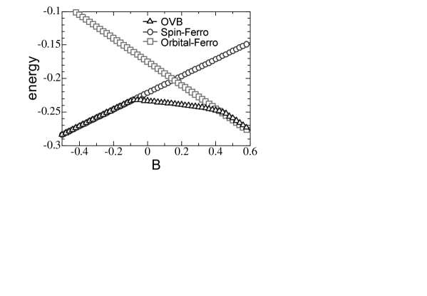
Fig.  1: The energy per site as a function of the exchange parameter $B$ for $A=D=0$; the ground-state energy obtained by the DMRG is shown by triangles. We also plot the energy computed for the spin-ferromagnetic state (circles) and the orbital-ferromagnetic state (squares). We clearly see two cusp structures, indicating first-order phase transitions. The intermediate region is identified as the OVB solid state.

In Fig. 1, the energy obtained by the DMRG is shown as a function of $B$ with keeping $A=0$ fixed. We find two first-order transition points; $B_{c1}\simeq-0.09$ and $B_{c2}\simeq 0.41$. As clearly seen in Fig. 1, the system favors the spin-ferromagnetic state for small $B$ ($<B_{c1}$), but stabilizes the OVB solid state${}^{\hbox{\immediate{?})}}$ for the intermediate region ($B_{c1}<B<B_{c2}$). For large $B$ ($>B_{c2}$), the ground state is in the orbital-ferromagnetic phase.

By repeating similar estimations of the critical points for other choices of $A$, we determine the ground-state phase diagram for $D=0$ in the $A$-$B$ plane, which is shown in Fig. 2. The phase diagram consists of four phases; the OVB phase (I), the spin-ferromagnetic phase (II), the orbital-ferromagnetic phase (III), and the spin-ferro/orbital-ferromagnetic phase (IV). We can estimate the phase boundary exactly in several limiting cases. First, by dropping the spin (orbital) degrees of freedom when the spin- (orbital-) ferromagnetic ground state is stabilized, we immediately find that the phase boundaries of II-IV and III-IV are exactly given by $A=-1$ and $B=-1$, respectively. We can also determine the exact asymptotic behavior of the boundary. The boundary between the phases I and II approaches $B=4|\epsilon_{g}^{(1/2)}|$ for $A\rightarrow\infty$, where $\epsilon_{g}^{(1/2)}=-\log 2+1/4\sim-0.443$ is the exact ground-state energy for the isotropic $T=1/2$ Heisenberg chain.${}^{\hbox{\immediate{\bf{?}})}}$ On the other hand, for $B\rightarrow\infty$, the I-III boundary approaches $A=|\epsilon_{g}^{(1)}|$, where $\epsilon_{g}^{(1)}\sim-1.401484$ is the ground-state energy for the $S=1$ Haldane chain.${}^{\hbox{\immediate{?})}}$ This asymptotic analysis is consistent with our phase diagram obtained here numerically.

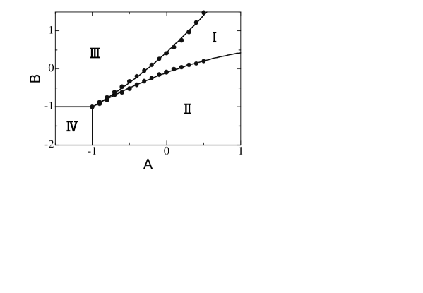
Fig.  2: Phase diagram of the 1D $S=1$ spin-orbital model in the $A$-$B$ plane without uniaxial single-ion anisotropy. The phase I is the OVB phase (see text). In the phase II, the spin part is in the fully polarized state while the orbital part forms the gapless antiferromagnetic $T=1/2$ Heisenberg chain. On the other hand, in the phase III, the orbital sector is in the ferromagnetic phase while the spin sector is in the $S=1$ Haldane phase. Both of the spin and orbital parts are in the fully polarized ferromagnetic states in the phase IV. All the transitions are of first order.

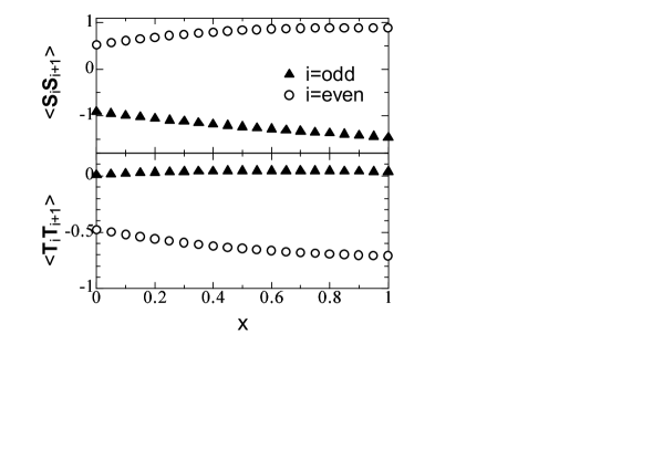
Fig.  3: Spin (upper panel) and orbital (lower panel) correlation functions in the phase I along the $A=B(=x)$ line in the OVB phase. The site index $i$ is even (odd) for open circles (solid triangles). The even-odd $i$-dependence reflects a dimer property of the OVB phase. With increasing $x$, the dimerization gets strong and the size of a gap becomes large.

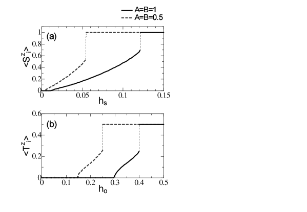
Fig.  4: Spin (a) and orbital (b) magnetization curves at $A=B=1$ (solid line) and 0.5 (dashed line). We calculate the spin (orbital) magnetization by setting $h_{o}=0(h_{s}=0)$. Note that both of the spin and orbital magnetizations exhibit typical behavior of gapful systems, although the orbital gap is much larger than the spin gap. For higher fields, the spin and orbital magnetizations show the first-order phase transition to the fully polarized state, which is signaled by a discontinuous jump.

Although characteristic properties of the phases II, III and IV can be directly deduced from those of the $S=1/2,1$ chains, there appear nontrivial properties due to the interplay of spins and orbitals in the OVB phase I. We thus calculate the short-range spin and orbital correlation functions by taking the line $A=B(=x)$ as representative parameters in the OVB phase.

The results are shown in Fig. 3. As $x$ increases, the even-odd $i$-dependence of the correlation functions gets stronger both for spin and orbital sectors, implying that the system favors the dimerization. At $x=1$, the orbital sector forms nearly perfect dimer singlets. i.e. $\langle{\bf T}_{i}\cdot{\bf T}_{i+1}\rangle\sim-3/4$ for even $i$, while it is almost zero for odd $i$. On the other hand, two adjacent spins are almost parallel for even $i$, i.e. $\langle{\bf S}_{i}\cdot{\bf S}_{i+1}\rangle\sim 1$, while for odd $i$, there are weak antiferromagnetic correlations. These properties clearly characterize the dimer-like nature of the OVB phase.${}^{\hbox{\immediate{?},\penalty 1000\hskip 0.91003pt plus 0.70004pt minus 0.70004pt{?},\penalty 1000\hskip 0.91003pt plus 0.70004pt minus 0.70004pt{?})}}$ It is remarkable that even if $x$ decreases from unity, the orbital correlation $\langle{\bf T}_{i}\cdot{\bf T}_{i+1}\rangle$ for odd $i$ stays very small, indicating that the orbital sector can be regarded as an assembly of approximately independent dimers irrespective of the values of $x$.

In order to observe the properties of the phase I in more detail, we compute the spin/orbital magnetization. To this end, we add the following terms to the Hamiltonian (1),

$${\cal H}_{ex}=-h_{s}\sum_{i}S_{i}^{z}-h_{o}\sum_{i}T_{i}^{z},$$ (2)

where $h_{s}$ and $h_{o}$ are external fields conjugate to the spin and orbital magnetizations. The calculated magnetization curves are shown in Fig. 4 for two typical choices of the exchange couplings. Let us first observe the spin magnetization for $x=A=B=1$ shown in Fig. 4(a). The magnetization $\langle{S_{i}^{z}}\rangle$ is zero in small fields, in accordance with the existence of a spin gap in the OVB phase. After the spin gap disappears at very low fields, the magnetization increases smoothly, and jumps at the second critical point (e.g. $h_{s}\sim 0.122$ for $x=1$), driving the system to the spin-ferromagnetic state via a first-order transition. Similarly, the orbital magnetization shown in Fig. 4(b) indicates that the OVB state with $\langle{T_{i}^{z}}\rangle=0$ is favored in small fields, and then the orbital magnetization $\langle{T_{i}^{z}}\rangle$ develops gradually beyond a critical field corresponding to the orbital gap. The system further undergoes a first-order transition to the orbital-ferromagnetic state. Comparing the spin and orbital gaps, we notice that the orbital gap is much larger than the spin gap, ${}^{\hbox{\immediate{?},\penalty 1000\hskip 0.91003pt plus 0.70004pt minus 0.70004pt{?})}}$ consistent with the results for correlation functions, where the orbital-dimerization is quite strong. In contrast to the low-field behavior, both spin and orbital degrees of freedom change their characters at the first-order transition points. Note that the resulting high-field phase with the fully spin (orbital) polarized state is the same as the phase II (III).

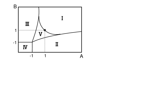
Fig.  5: Phase diagram of the $S=1/2$ spin-orbital model. ${}^{\hbox{\immediate{?},\penalty 1000\hskip 0.91003pt plus 0.70004pt minus 0.70004pt{?},\penalty 1000\hskip 0.91003pt plus 0.70004pt minus 0.70004pt{?},\penalty 1000\hskip 0.91003pt plus 0.70004pt minus 0.70004pt{?})}}$ Phase I is a gapful phase with doubly degenerate ground states which form alternating spin and orbital singlets. In the phase II, the spin degrees of freedom are in the fully polarized ferromagnetic state while the orbitals are in the antiferromagnetic ground state and vice versa in the phase III. Both spin and orbital degrees of freedom are in the fully polarized ferromagnetic states in the phase IV. The phase V is a gapless phase including an integrable SU(4) point ($A=B=1$).

Before closing this section, we compare the present phase diagram with that for the $S=1/2$ spin-orbital model,${}^{\hbox{\immediate{?},\penalty 1000\hskip 0.91003pt plus 0.70004pt minus 0.70004pt{?},\penalty 1000\hskip 0.91003pt plus 0.70004pt minus 0.70004pt{?},\penalty 1000\hskip 0.91003pt plus 0.70004pt minus 0.70004pt{?})}}$ which is sketched in Fig. 5. The corresponding spin-orbital Hamiltonian is given by (1) by putting $S=1/2$ and replacing $A$ with $A/4$ for the spin sector. Overall features are similar both in $S=1$ and $1/2$ models: the phases II, III and IV are respectively characterized by the spin-ferro/orbital-singlet state, the spin-singlet/orbital-ferro state and the spin-ferro/orbital-ferro state. The phase I also exhibits similar dimer-like properties in both cases. A remarkable difference is the gapless phase V realized in the $S=1/2$ model around the SU(4) point. This phase, which is stabilized by enhanced quantum fluctuations both in spin and orbital degrees of freedom, disappears in the $S=1$ model. We think that the phase V is inherent in the $S=1/2$ case, and a higher-spin extension of the SU(2)$\otimes$SU(2) model may have a phase diagram similar to the present $S=1$ case.

In contrast to the $S=1/2$ model, the single ion anisotropy plays an important role for the $S=1$ model, which may provide a rich phase diagram. This problem is addressed in the following.

4 Effects of Uniaxial Single-Ion Anisotropy

4.1 $D<0$

Let us now consider the effects of uniaxial single-ion anisotropy. We start with the ground-state properties for the case of $D<0$.

Recall that in the phases II and IV in Fig. 2, the spin sector is in the fully-polarized state, so that the nature of these phases may not be altered upon the introduction of $D<0$, except that the direction of spin ordering is now fixed to the $z$-axis. On the other hand, the negative $D$ suppresses quantum fluctuations in the spin-gap phases I and III, resulting in the antiferromagnetic spin order with $Z_{2}$ symmetry breaking. We refer to the corresponding new ordered phases as the phase I_m and III_m, respectively.

Note that different types of spin order should emerge in the phases I_m and III_m. The spin-antiferromagnetic order has the 4-site period (up-up-down-down alignment) in the phase I_m, and the 2-site period (up-down-up-down alignment) in the phase III_m, as schematically shown in Fig. 6. This difference comes from the ground-state properties without anisotropy. Namely, in the OVB phase I, spins favor a ferromagnetic configuration in a orbital-dimer singlet and an antiferromagnetic configuration between adjacent orbital singlets, so that the spin sector is described by an effective ferro-antiferromagnetic bond-alternating chain. On the other hand, in the phase III_m, the spin sector forms the $S=1$ Haldane state at $D=0$, so that it naturally leads to an ordinary antiferromagnetic order upon the introduction of $D<0$.

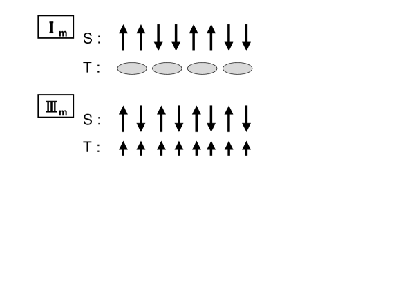
Fig.  6: Schematic description of spin orders for the phases I_m and III_m. The label S (T) denotes the spin (orbital) part, respectively.

The above tendency to spin ordering is indeed observed in the nearest-neighbor correlation functions shown in Fig. 7 as a function of $D(<0)$. We exploit two typical values of $A$ and $B$, which correspond to the parameters for the phases I and III at $D=0$. Even in the presence of $D$, both spin and orbital correlation functions show (do not show) the even-odd $i$-dependence for the parameters corresponding to the phase I_m (III_m). It should be also noticed that the orbital correlations are almost independent of $D$, as should be naively expected: almost isolated orbital-dimer states are favored in the phase I_m, while the orbital sector is always in the fully polarized state, $\langle{\bf T}_{i}\cdot{\bf T}_{i+1}\rangle=1/4$, in the phase III_m .

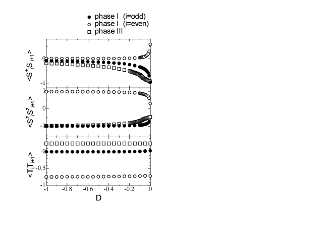
Fig.  7: Spin (upper and middle panels) and orbital (lower panel) correlation functions as a function of $D$: $A=B=1$ (solid circles : $i=odd$ and open circles : $i=even$) and $A=-1$, $B=1$ (open squares).

As mentioned above, the spin-antiferromagnetic order with the 4 (2)-site period should be stabilized beyond a certain critical value of $|D|$ in the phase I_m (III_m). Therefore, spin fluctuations are suppressed and thus the correlation $\langle S^{z}_{i}\cdot S^{z}_{i+1}\rangle\rightarrow\pm 1$ while $\langle S^{+}_{i}\cdot S^{-}_{i+1}\rangle\rightarrow 0$ as $|D|$ increases. We now determine the phase transition point for III$\rightarrow$III_m. Note that the orbital sector always orders ferromagnetically, so that the Hamiltonian (1) for the spin sector is reduced to

$${\cal H}_{\it OF} = J^{\prime}\sum_{i}\left({\bf S}_{i}\cdot{\bf S}_{i+1}+A\right)+D\sum_{i}\left(S_{i}^{z}\right)^{2},$$ (3)

with $J^{\prime}=J(1+B)/4$. In this case, the competition of the single-ion anisotropy $D$ and the effective exchange-coupling $J^{\prime}$ results in the following transition, which is independent of $A$. According to the results for the isotropic $S=1$ chain, ${}^{\hbox{\immediate{\bf{?}},\penalty 1000\hskip 0.91003pt plus 0.70004pt minus 0.70004pt{\bf{?}},\penalty 1000\hskip 0.91003pt plus 0.70004pt minus 0.70004pt{\bf{?}},\penalty 1000\hskip 0.91003pt plus 0.70004pt minus 0.70004pt{\bf{?}})}}$ the ground state is in the Haldane phase for $-0.35J^{\prime}{\leq}D{\leq}J^{\prime}$, and in the Ne$\grave{e}$l phase for $D<-0.35J^{\prime}$. Therefore, the critical value is given by $D_{c}=-0.175J$ in Fig. 7, which separates the Haldane phase and Ne$\grave{e}$l phase for the spin sector.

It is more difficult to determine the boundary between I and I_m only from our data for the correlation functions in Fig. 7, partially because the spin gap is very small in the phase I. Nevertheless, by taking into account that the spin gap is much smaller than the orbital gap (Fig. 4), we reasonably expect that the corresponding critical value of $D$, which separates I and I_m in Fig. 7, may be quite small, say, less than $-0.1$. The precise critical value should be obtained by exploiting improved numerical methods, which we wish to leave for the future study.

We show the phase diagram in the $A$-$B$ plane for $D<0$ in Fig. 8. Since the transition from the OVB phase to the other phases is of first order, we determine the corresponding boundary by comparing three-types of the energy among the OVB solid state, the spin-ferromagnetic state and the orbital-ferromagnetic state. As mentioned above, the phase boundary between the phases III and III_m is given by

$$B_{c}\simeq-11.4D-1,$$ (4)

which is independent of $A$. For example, $B_{c}\simeq 0.14$ for $D=-0.1$, as shown in Fig. 8(a). In the case of $D=-1.0$ in Fig. 8(b), the phase III_m dominates the phase III in the displayed region, because the boundary between these two phases is at $B_{c}\simeq 10.4$ for $D=-1.0$. Note that the orbital sector orders ferromagnetically for all $D$ in the phases III, III_m and IV. As mentioned above, the spin state in the OVB phase I is sensitive to $D$, so that the ordered phase I_m dominates the phase I both for $D=-0.1$ and $-1.0$ in the region shown in Fig. 8

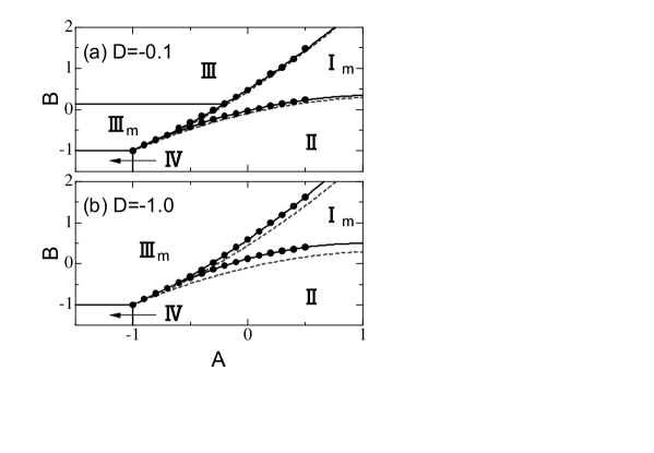
Fig.  8: Phase diagrams for $D<0$: (a)$D=-0.1$ and (b)$D=-1.0$. The phases labeled as II, III and IV are the same as in Fig. 2. I_m and III_m are spin-ordered phases (see text). The solid lines except for the III-III_m boundary represent first-order transitions. For reference, the phase boundary at $D=0$ is shown by the dashed lines.

4.2 $D>0$

Let us now move to the positive $D$ case. We start with the phases III and IV, for which the phase transition points are easily determined, since the orbital sector is in the fully polarized state. In the phase III, the so-called large-$D$ phase is stabilized in the spin sector for $D>J^{\prime}=J(1+B)/4$; i.e. for $-1<B<B_{c}$ ($B_{c}=-1+4D$), the large-$D$ phase appears, while the Haldane phase persists for $B>B_{c}$. On the other hand, in the phase IV, the XY phase emerges ${}^{\hbox{\immediate{?},\penalty 1000\hskip 0.91003pt plus 0.70004pt minus 0.70004pt{\bf{?}},\penalty 1000\hskip 0.91003pt plus 0.70004pt minus 0.70004pt{\bf{?}})}}$ in the region $-1-4D<B<-1$ in the presence of the $D$-term.

It turns out that the boundary between the phases I and II is quite sensitive to positive $D$, and exhibits somewhat complicated features. This is contrasted to the robust first-order transition between the phases I and III, which hardly changes its character as far as $D$ is small. To make the above point clear, we observe the behavior of the correlation functions by choosing $D=0.01$ with two typical values of $A=0$ and 0.5. In Fig. 9 (a), the $B$-dependence of the spin and orbital correlation functions are shown for $A=0$. For small $B$, the ground state is in the phase II, so that both spin and orbital correlation functions are spatially uniform without the even-odd $i$-dependence. With increasing $B$, a continuous quantum phase transition occurs from the phase II to I at $B_{c}\sim-0.1$, in contrast to the first-order transition at $D=0$, as seen in Fig. 9(a). Beyond the critical value $B_{c}$, the spin and orbital correlation functions exhibit the even-odd $i$-dependence, reflecting dimer properties of the OVB solid state. Unfortunately, we cannot figure out whether this continuous transition is Berezinskii-Kosterlitz-Thouless (BKT) type ${}^{\hbox{\immediate{\bf{?}},\penalty 1000\hskip 0.91003pt plus 0.70004pt minus 0.70004pt{\bf{?}},\penalty 1000\hskip 0.91003pt plus 0.70004pt minus 0.70004pt{\bf{?}})}}$ or not only from the results shown in Fig. 9, because an extremely large system size is necessary to obtain the sensible results in our spin-orbital model with a tiny spin gap. Nevertheless, we can discuss some characteristic properties of each phase from the correlation functions. First, we note that the spin sector in the phase II may be changed to the XY phase upon introduction of $D$.${}^{\hbox{\immediate{?},\penalty 1000\hskip 0.91003pt plus 0.70004pt minus 0.70004pt{?},\penalty 1000\hskip 0.91003pt plus 0.70004pt minus 0.70004pt{?})}}$ This can be inferred from the spin correlation functions shown in Fig. 9, which indeed show the preference of the XY phase: $\langle S^{+}_{i}S^{-}_{i+1}\rangle\sim 1$ and $\langle S^{z}_{i}S^{z}_{i+1}\rangle\sim 0$. This observation is also supported by the following consideration. Note first that the orbital correlation function is not affected by $D$ in the phase II, and takes the constant value $\langle{\bf T}_{i}\cdot{\bf T}_{i+1}\rangle\sim\epsilon_{g}^{(1/2)}$ characteristic of the $T=1/2$ orbital chain, so that we can focus on the remaining $S=1$ spin part. According to the isotropic $S=1$ ferromagnetic chain,${}^{\hbox{\immediate{?},\penalty 1000\hskip 0.91003pt plus 0.70004pt minus 0.70004pt{?},\penalty 1000\hskip 0.91003pt plus 0.70004pt minus 0.70004pt{?})}}$ the first-order phase transition from the spin-ferromagnetic phase to the XY phase occurs upon introducing $D$, which is consistent with our numerical results for the correlation functions.

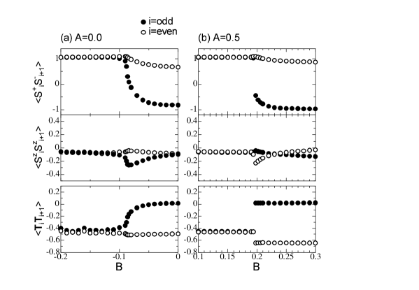
Fig.  9: Spin (upper and middle panels) and orbital (lower panel) correlation functions for $D=0.01$ as a function of $B$ ((a) $A=0.0$, (b) $A=0.5$). The site index $i$ is even (open circle) or odd (solid circle). The even-odd $i$-dependence reflects dimer properties of the phase I.

The above continuous transition is in contrast to that for $A=0.5$ shown in Fig. 9 (b), where the system exhibits the first-order phase transition accompanied by a clear jump at $B_{c}\sim 0.2$ both in the spin and orbital correlation functions. This characteristic behavior is essentially the same as that for $D=0$.

By examining the correlation functions for other choices of $A$, we end up with a phase diagram expected for $D=0.01$, which is shown in Fig. 10. The phase boundary between the phases I and II is either continuous or first-order depending on the value of $A$: the transition is continuous (first-order) for $A<0.1$ ($A>0.1$). We have checked that the critical value of $A$, which separates these two types of transitions, increases monotonically with the increase of $D$. For example, the critical value is $A=0.5$ for $D=0.012$. For small $D$, the first-order transition dominates most part of the I-II phase boundary.

Here, an important question arises: what really causes the change in the nature of the transitions, first-order or continuous, on the I-II phase boundary. To address this question, we should go into the detail of the phase I. Since the orbital part always forms the dimerized state in the phase I even for finite $D$, we again focus on the spin sector. Recall here that the spin sector in the OVB phase I forms the state similar to the $S=2$ Haldane-gap state (same universality class).${}^{\hbox{\immediate{?},\penalty 1000\hskip 0.91003pt plus 0.70004pt minus 0.70004pt{?})}}$ Fortunately, the 1D $S=2$ Haldane system with uniaxial single-ion anisotropy was already investigated.${}^{\hbox{\immediate{\bf{?}},\penalty 1000\hskip 0.91003pt plus 0.70004pt minus 0.70004pt{\bf{?}})}}$ Schollwöck numerically checked the disappearance of the spin gap at a very small critical value of $D$ ($\sim 0.02J$), and the system enters the ”intermediate-$D$ phase”, which was claimed to be equivalent with the XY-phase.${}^{\hbox{\immediate{?})}}$ Immediately after the above analysis, Oshikawa found that the behavior of the string correlation in $z$-axis deviates from a simple power-law, as a result, he suggested that this intermediate-$D$ phase is not truly gapless XY-phase, but somewhat modified one with some anomalous properties in the $z$-components. ${}^{\hbox{\immediate{?})}}$ Anyway, the message from the above analysis is that the introduction of small positive $D$ changes the Haldane phase to the so-called intermediate-$D$ phase. In our model, the size of the spin gap in the phase I gets small as $A\rightarrow-1$ and $B\rightarrow-1$ (Fig. 4). Therefore, we think that the spin sector in the OVB phase is changed to the ”intermediate-$D$ type phase” in the region with small $A$ and $B$, while the original spin-gap state in the OVB phase can still persist for larger $A$ and $B$. This may cause the change in the nature of the phase transition on the I-II phase boundary. Unfortunately, our numerical calculation is not powerful enough to draw a definite conclusion about the existence of the ”intermediate-$D$ type phase”. We would like to clarify the detail in the future work.

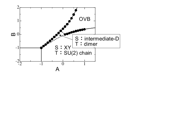
Fig.  10: Phase diagram for the model with $D=0.01$. The solid lines (with dots) indicate the first-order transition. Concerning the phase boundary between I and II, there is a continuous transition (broken line) for $A\leq 0.1$, and a first-order transition (solid line with dots) for $A>0.1$. The intermediate-$D$ phase is expected to emerge in the spin sector of the OVB phase for small $A$ and $B$. Note also that around the boundary of $B=-1$, there appear two new spin phases: the large-$D$ phase (XY spin phase) in the tiny region $-1<B<-0.96$ ($-1.04<B<-1$), although not shown explicitly in the figure (see text).

5 Summary

We have investigated quantum phase transitions of the 1D $S=1$ spin-orbital model with uniaxial single-ion anisotropy. By means of the DMRG method, we have calculated the ground-state energy, the spin/orbital magnetizations, and the correlation functions, from which we have determined the zero-temperature phase diagram.

In the absence of the anisotropy, there appear four phases including the OVB phase characteristic of the $S=1$ spin-orbital system. ${}^{\hbox{\immediate{?})}}$ This phase has a small spin gap and a fairly large orbital gap. In comparison with the $S=1/2$ spin-orbital model, we have found that most of the phase diagram shows similar properties, but the phase V inherent in the $S=1/2$ model disappears in the $S=1$ case. We believe that a higher spin extension of the model should have the phase diagram similar to that of the present $S=1$ model.

The introduction of uniaxial single-ion anisotropy $D$ gives rise to some interesting aspects. For negative $D$, two different types of magnetic orders appear, depending on whether the system at $D=0$ is in the orbital-ferromagnetic phase or the OVB phase. Since the spin gap for the OVB phase is much smaller than that for the orbital-ferromagnetic phase, the spin order in the OVB phase is induced even in the small $|D|$ region.

On the other hand, it has turned out that the situation is much more subtle in the positive $D$ case. In particular, the phase transition between the OVB phase I and the spin-ferromagnetic phase II exhibits somewhat complicated feature: the nature of transition changes from first-order to continuous one, depending sensitively on the value of $D$. Although we have not been able to obtain the precise phase diagram, some characteristic properties of each phase have been discussed on the basis of the correlation functions. These nontrivial properties originate from interplay of the spin and orbital degrees of freedom, which may exemplify interesting aspects of the spin-orbital systems. Further investigations should be done in the future study, especially for the positive $D$ case.

References

- [1] I. Affleck: Nucl. Phys. B 265 (1986) 409.
- [2] B. Sutherland: Phys. Rev. B 12 (1975) 3795.
- [3] T. Itakura and N. Kawakami: J. Phys. Soc. Jpn. 64 (1995) 2321.
- [4] Y. Yamashita, N. Shibata, and K. Ueda: Phys. Rev. B 58 (1998) 9114.
- [5] S. K. Pati, R. R. P. Singh, and D. I. Khomskii: Phys. Rev. Lett. 81 (1998) 5406.
- [6] P. Azaria, A. O. Gogolin, P. Lecheminant, and A. A. Nersesyan: Phys. Rev. Lett. 83 (1999) 624; P. Azaria, E. Boulat, and P. Lecheminant: Phys. Rev. B 61 (2000) 12112.
- [7] Y. Yamashita, N. Shibata, and K. Ueda: J. Phys. Soc. Jpn. 69 (2000) 242; Y. Tsukamoto, N. Kawakami, Y. Yamashita and K. Ueda: Physica B 281-282 (2000) 540.
- [8] C. Itoi, S. Qin, and I. Affleck: Phys. Rev. B. 61 (2000) 6747.
- [9] G. Khaliullin, P. Horsch, and A. M. Oleś: Phys. Rev. Lett. 86 (2001) 3879.
- [10] S.-Q. Shen, X. C. Xie, and F. C. Zhang: Phys. Rev. Lett. 88 (2002) 027201.
- [11] J. Sirker and G. Khaliullin: Phys. Rev. B 67 (2003) 100408.
- [12] P. Horsch, G. Khaliullin, and A. M. Oleś: Phys. Rev. Lett. 91 (2003) 257203.
- [13] S. Miyashita, A. Kawaguchi, N. Kawakami and G. Khaliullin: Phys. Rev. B 69 (2004) 104425.
- [14] C. Ulrich, G. Khaliullin, J. Sirker, M. Reehuis, M. Ohl, S. Miyasaka, Y. Tokura, and B. Keimer: Phys. Rev. Lett. 91 (2003) 257202.
- [15] S. R. White: Phys. Rev. Lett. 69 (1992) 2863; Phys. Rev. B. 48 (1993) 10345.
- [16] H. Bethe: Z. Phys. 71 (1931) 205; L. Hulthen: Arkiv. Math. Astro. Fys. 26A (1938) 938.
- [17] T. Tonegawa, T. Nakao and M. Kaburagi: J. Phys. Soc. Jpn. 65 (1996) 3317.
- [18] W. Chen, K. Hida and B. C. Sanctuary: J. Phys. Soc. Jpn. 69 (2000) 237; Phys. Rev. B 67 (2003) 104401.
- [19] A. Koga: Phys. Lett. A 296 (2002) 243.
- [20] T. Hikihara: J. Phys. Soc. Jpn. 71 (2002) 319.
- [21] H. J. Schultz: Phys. Rev. B 34 (1986) 6372.
- [22] M. den Nijs and K. Rommelse: Phys. Rev. B 40 (1989) 4709.
- [23] V. L. Berezinskii: Zh. Eksp. Teor. Fiz. 61 (1971) 1144 [Sov. Phys. JETP 34 (1972) 610].
- [24] J. M. Kosterlitz and D. J. Thouless: J. Phys. C 6 (1973) 1181.
- [25] J. B. Kogut: Rev. Mod. Phys. 51 (1979) 659.
- [26] M. Oshikawa: J. Phys.: Condens. Matter 4 (1992) 7469; M. Oshikawa, M. Yamanaka and S. Miyashita: cond-mat/9507098 (unpublished)
- [27] U. Schollwöck, O. Golinelli and T. Jolicoeur: Phys. Rev. B 54 (1996) 4038.