Kinetic Theory of dilute gases under nonequilibrium conditions

Abstract

The significance of the recent finding of the velocity distribution function of the steady-state Boltzmann equation under a steady heat current obtained by Kim and Haykawa (J. Phys. Soc. Jpn. 72, 1904 (2003)) is discussed. Through the stability analysis, it seems that the steady solution is stable. One of possible applications to the nonequiliburium Knudsen effect in which one cell at equilibrium is connected to another cell under the steady heat conduction is discussed. This solution apparently shows that steady-state thermodynamics proposed by Sasa and Tasaki cannot be used in a naive setup. The preliminary result of our simulation based on molecular-dynamics for nonequilibrium Knudsen effect is also presented to verify the theoretical argument.

I Introduction

Kinetic theory of dilute gases has played crucial roles in the history of nonequilibrium statistical mechanics. The theoretical treatment of linear transport problems is well established including the derivation of Navier-Stokes equation and the relation between Boltzmann equation and the linear-response theory through a number of studies of Boltzmann equation[1, 2, 3].

The transport problems under the nonlinear-nonequilibrium circumstance, however, is still controversial. In fact, we know Burnett’s classical work in which he obtained an approximate hydrodynamic equation at the second order nonequilibrium condition[4], but we realize that hydrodynamic equation he obtained is unstable for perturbations[5, 6]. Therefore, one may suggest that the validity of Chpaman-Enskog method is so limited that we should use Grad expansion[7] to discuss the higher order perturbations such as Burnett order and super-Burnett order[6]. On the other hand, when we obtain the steady solution of Burnett equation, the stability of the steady inhomogeneous solution may be different from that of dynamical Burnett equation for homogeneous perturbation. Therefore we cannot judge whether the calculation at Burnett order based on Chapman-Enskog method is useless even when Burnett’s hydrodynamic equation is unstable. Unfortunately, these difficulties might be regarded as unimportant, because the solution at Burnett order is practically useless except for few cases such as the analysis of shock waves.

In these days, however, the solution of Boltzmann equation at Burnett order has attracted much interest among researchers who try to extend the linear nonequilibrium statistical mechanics to nonlinear nonequilibrium statistical mechanics[8, 9]. In fact, since all of attempts are formulated to match them with the linear response theory, their consistency with nonlinear theory like Burnett solution should be important.

Recently, Kim and Hayakawa[10] have extended Burnett’s classical work on Boltzmann equation and obtained the explicit steady solution of Boltzmann equation under the steady heat conduction at second (Burnett) order. The accuracy and numerical stability of this solution is confirmed by Fushiki[11] from his molecular-dynamics simulation. This stable behavior does not contradict with blown-up tendency of Burnett equation for perturbation of short wavelength or high frequency, because the simulation does not involve any perturbation with short wavelength or high frequency. Their solution is useful[12] to examine the validity of nonequilibrium theories such as information theory[8] and the steady-state thermodynamics (SST)[9] based on thermodynamic arguments. They also succeed to apply the solution to calculate the rate of chemical reaction under the nonequilibrium circumstance in which the linear nonequilibrium effects are canceled from the consideration of symmetries[13].

The purpose of this paper is to (i) summarize the achievement of Kim and Hayakawa, (ii) to discuss the stability of the steady solution at Burnett order, and (iii) to introduce the result of the molecular-dynamics (MD) simulation for nonequilibrium Knudsen effect to examine SST.

The organization of this paper is as follows. In the next section, we briefly summarize the outline of the solution obtained by Kim and Hayakawa[10]. In section III, we will discuss the stability of the solution. In section IV, we will discuss Knudsen effect under a nonequilibrium condition based on MD simulation.

II The outline of the solution by Kim and Hayakawa

In this section, we briefly summarize the solution of steady Boltzmann equation under the heat conduction obtained by Kim and Hayakawa[10]. Suppose a system of dilute gas in a steady state whose velocity distribution function is $f_{\mathrm{1}}=f({\bf r},{\bf v}_{\mathrm{1}})$. The steady state Boltzmann equation is written as

$${\bf v}_{\mathrm{1}}\cdot\nabla f_{\mathrm{1}}=J(f_{\mathrm{1}},f_{\mathrm{2}}),$$ (1)

where the collision integral $J(f_{\mathrm{1}},f_{\mathrm{2}})$ for hard core molecules is expressed as

$$J(f_{\mathrm{1}},f_{\mathrm{2}})=\int\int\int(f^{\prime}_{\mathrm{1}}f^{\prime}_{\mathrm{2}}-f_{\mathrm{1}}f_{\mathrm{2}})gbdbd\epsilon d{\bf v}_{\mathrm{2}}.$$ (2)

Here the velocity distribution $f_{\mathrm{1}}$ and $f_{\mathrm{2}}$ change to $f^{\prime}_{\mathrm{1}}$ and $f^{\prime}_{\mathrm{2}}$ by a binary collision. The relative velocity of the two molecules before and after the interaction has the same magnitude $g=|{\bf v}_{\mathrm{1}}-{\bf v}_{\mathrm{2}}|$. The relative position of the two molecules is represented by the impact parameter $b$ and $\epsilon$ which represents the angle of the plane to which $g$ and $g^{\prime}$. The impact parameter $b$ is identical to explicitly determined by specifying the kind of molecules.

The velocity distribution function $f_{\mathrm{1}}$ can be expanded as:

$$f_{\mathrm{1}}=f^{(0)}_{\mathrm{1}}+f^{(1)}_{\mathrm{1}}+f^{(2)}_{\mathrm{1}}+\cdots=f^{(0)}_{\mathrm{1}}(1+\phi^{(1)}_{\mathrm{1}}+\phi^{(2)}_{\mathrm{1}}+\cdots),$$ (3)

where the small parameter of the perturbation is Knudsen number , i.e. mean free path of the molecules is much less than the characteristic length of the change of macroscopic variables. $f^{(0)}_{\mathrm{1}}$ in eq.(3) is the local Maxwellian distribution function written as

$$f^{(0)}_{\mathrm{1}}=n({\bf r})\left(\frac{m}{2\pi T({\bf r})}\right)^{\frac{3}{2}}\exp[-\frac{m{\bf v}_{\mathrm{1}}^{2}}{2T({\bf r})}],$$ (4)

where $m$ is mass of the molecules. $n({\bf r})$ and $T({\bf r})$ denote the density and the temperature at position ${\bf r}$, respectively. Substituting eq.(3) into the steady state Boltzmann equation (1), we arrive at the following set of equations:

$$L[f^{(0)}_{\mathrm{1}}]\phi^{(1)}_{\mathrm{1}}={\bf v}_{\mathrm{1}}\cdot\nabla f^{(0)}_{\mathrm{1}},$$ (5)

for $O(K)$ and

$$L[f^{(0)}_{\mathrm{1}}]\phi^{(2)}_{\mathrm{1}}={\bf v}_{\mathrm{1}}\cdot\nabla f^{(1)}_{\mathrm{1}}-J(f^{(1)}_{\mathrm{1}}f^{(1)}_{\mathrm{2}}),$$ (6)

for $O(K^{2})$, where the linear integral operator $L[f^{(0)}_{\mathrm{1}}]$ is defined as

$$L[f^{(0)}_{\mathrm{1}}]X_{\mathrm{1}}\equiv\int\int\int f^{(0)}_{\mathrm{1}}f_{\mathrm{2}}^{(0)}(X_{\mathrm{1}}^{\prime}-X_{\mathrm{1}}+X^{\prime}_{\mathrm{2}}-X_{\mathrm{2}})gbdbd\epsilon d{\bf v}_{\mathrm{2}}.$$ (7)

It is important to consider the solubility conditions of these integral equations, for the steady state Boltzmann equation, which are given by

$$\int\Phi_{i}{\bf v}_{\mathrm{1}}\cdot\nabla f^{(0)}_{\mathrm{1}}d{\bf v}_{\mathrm{1}}=0,$$ (8)

for $O(K)$, where $\Phi_{i}$ is one of the collision invariants:

$$\Phi_{1}=1,\quad\Phi_{2}=m{\bf v}_{\mathrm{1}},\quad\Phi_{3}=\frac{1}{2}m{\bf v}_{\mathrm{1}}^{2}.$$ (9)

Substituting eq.(4) into the solubility condition (8), it can be shown that $nT$ is uniform. We use this result in our calculation. The solubility condition for $O(K^{2})$ is given by

$$\int\Phi_{i}{\bf v}_{\mathrm{1}}\cdot\nabla f^{(1)}_{\mathrm{1}}d{\bf v}_{\mathrm{1}}=0.$$ (10)

To make the solutions of the integral equations (6) and (7) definite, five further conditions must be specified; we identify the density:

$$n({\bf r})=\int f_{\mathrm{1}}d{\bf v}_{\mathrm{1}}=\int f^{(0)}_{\mathrm{1}}d{\bf v}_{\mathrm{1}},$$ (11)

the temperature:

$$\frac{3n({\bf r})T({\bf r})}{2}=\int\frac{m{\bf v}_{\mathrm{1}}^{2}}{2}f_{\mathrm{1}}d{\bf v}_{\mathrm{1}}=\int\frac{m{\bf v}_{\mathrm{1}}^{2}}{2}f^{(0)}_{\mathrm{1}}d{\bf v}_{\mathrm{1}},$$ (12)

and the mean flow:

$$n({\bf r}){\bf u}({\bf r})=\int{\bf v}_{\mathrm{1}}f_{\mathrm{1}}d{\bf v}_{\mathrm{1}}=\int{\bf v}_{\mathrm{1}}f^{(0)}_{\mathrm{1}}d{\bf v}_{\mathrm{1}}.$$ (13)

Here we assume that no mean flow ${\bf u}=0$ exists in the system.

Skipping the derivation of the solution at Burnett order, let us write the explicit form of the steady solution for hard core molecules as under the temperature gradient:

$$f=f^{(0)}[1 - \frac{4q_{x}}{5b_{11}nT}(\frac{m}{2T})^{\frac{1}{2}}\sum_{r\geq 1}r!b_{1r}c_{x}\Gamma(r+\frac{5}{2})S^{r}_{\frac{3}{2}}({\bf c}^{2})$$ (14)

$$+ \frac{4096mq_{x}^{2}}{5625b_{11}^{2}n^{2}T^{3}}\{\sum_{r\geq 2}r!b_{0r}\Gamma(r+\frac{3}{2})S^{r}_{\frac{1}{2}}({\bf c}^{2})$$ (15)

$$+ \sum_{r\geq 0}r!b_{2r}(2c_{x}^{2}-c_{y}^{2}-c_{z}^{2})\Gamma(r+\frac{7}{2})S^{r}_{\frac{5}{2}}({\bf c}^{2})\}],$$ (16)

where $b_{1r}$, $b_{0r}$ and $b_{2r}$ for $r\leq 7$ can be determined as listed in Tables.I. Note that we have confirmed the convergence of series $b_{kr}$ by changing $r$. Here $q_{x}$ represents $x-$component of the heat-flux in the cell on the right hand side in the nonequilibrium steady state which corresponds to the $x$ component of the heat flux in eq.(19). In eq.(16), $\Gamma(x)$ is the Gamma function, ${\bf c}={\bf v}\sqrt{m/2T}$, and $S^{p}_{k}(X)$ is the Sonine polynomial defined by

$$(1-\omega)^{-k-1}e^{-\frac{X\omega}{1-\omega}}=\sum_{p=0}^{\infty}\Gamma(p+k+1)S_{k}^{p}(X)\omega^{p}.$$ (17)

This kind of analysis, of course, is possible to two-dimensional dilute hard-core gases. Kim[14] has already obtained the result to compare his result with MD simulation.

In the derivation the solubility conditions for $O(K^{2})$ is important. Thus, eq.(10) leads to the condition:

$$\nabla\cdot{\bf q}^{(1)}=0,$$ (18)

where ${\bf q}^{(1)}$, i.e. the heat flux for $f^{(1)}_{\mathrm{1}}$ can be obtained as

$${\bf q}^{(1)}=\int^{\infty}_{-\infty}d{\bf v}_{\mathrm{1}}\frac{m{\bf v}_{\mathrm{1}}^{2}}{2}{\bf v}_{\mathrm{1}}f^{(1)}_{\mathrm{1}}=-b_{11}\frac{75}{64\sigma^{2}}\left(\frac{T}{\pi m}\right)^{\frac{1}{2}}\nabla T,$$ (19)

with $b_{11}$ listed in Table.I. It must be emphasized that ${\bf q}^{(2)}$ should satisfy

$${\bf q}^{(2)}=0$$ (20)

from the symmetry consideration of $f^{(2)}$. Thus, the solubility conditions for $f^{(2)}_{\mathrm{1}}$ of the steady state Boltzmann equation lead to the fact that the heat flux is constant to the second order. From eqs.(18) and (19), we also obtain an important relation between $\left(\nabla T\right)^{2}$ and $\nabla^{2}T$ as

$$\frac{\left(\nabla T\right)^{2}}{2T}+\nabla^{2}T=0.$$ (21)

From eq.(21), the term of $\nabla^{2}T$ can be replaced by the terms of $\left(\nabla T\right)^{2}$.

Amongst several applications of the solution, in this paper, we emphasize that the solution can examine the validity of SST proposed by Sasa and Tasaki[9]. They propose a non-trivial nonequilibrium effect in a simple setup as follows( Fig. 1). There are two cells whose size along $x$ axis is $L_{0}$. Both of the cells are filled with dilute gases and connected to each other by a small hole at $x=0$ whose linear dimension along $x$ axis and its diameter are less than the mean free path. The cell on the left hand side is at equilibrium of temperature $T_{0}$, while the cell on the right hand side is in a nonequilibrium steady state under a temperature gradient caused by the right wall at temperature $T_{1}$ at $x=L_{0}$ and the thin mid-wall at temperature $T_{0}$.

FIG. 1.: Setup of nonequilibrium Knudsen effect.

Sasa and Tasaki predicted the following results[9]. When the system shown in Fig.1 is in a steady state, the osmosis $\Delta P$

$$\Delta P \equiv P_{xx}-P_{0},$$ (22)

always positive, where $P_{0}$ is the pressure in the equilibrium cell and $P_{xx}$ is the $xx$-component of the pressure tensor $P_{ij}$ in the nonequilibrium cell which is defined by

$$P_{ij}=\int d{\bf v}m(v_{i}-u_{i})(v_{j}-u_{j})f({\bf v}).$$ (23)

In addition, there is a relation among $n(0)$, $P_{xx}$, $n_{0}$ and $P_{0}$ as

$$\frac{n(0)}{n_{0}}=\left(\frac{\partial P_{xx}}{\partial P_{0}}\right)_{T_{0},J},$$ (24)

where $n(0)$ is the density of the cell in the nonequilibrium steady state around the wall and $n_{0}$ is the density of the cell at equilibrium.

A nonequilibrium steady state is achieved when the mean mass flux at the hole is zero. Neglecting the Knudsen layer effect, i.e. the slip effect around the ’wall’[3, 15], we can calculate the balance of mass flux as

$$\int^{\infty}_{0}dv_{x}\int d^{2}v_{\bot}mv_{x}f_{0}+\int^{0}_{-\infty}dv_{x}\int d^{2}v_{\bot}mv_{x}f|_{x=0}=0,$$ (25)

where $v_{\bot}$ represents the components of the velocity which are orthogonal to $v_{x}$, i.e. $v_{y}$ and $v_{z}$. From eq.(25), we can obtain the relation between the density of the cell in the nonequilibrium steady state around the hole $n(0)$ and that of the cell at equilibrium $n_{0}$ as

$$n(0)=n_{0}[1+\lambda_{n}\frac{mJ_{x}^{2}}{n_{0}^{2}T^{3}}],$$ (26)

to the second order, where $\lambda_{n}\simeq 8.21\times 10^{-2}$ in the approximation until 7th order expansion of $b_{kr}$.

Similarly we can calculate pressure tensor $P_{ij}$ as

$$P_{ij} = nT[\delta_{ij}+\lambda_{P}^{ij}\frac{mJ_{x}^{2}}{n_{0}^{2}T^{3}}],$$ (27)

with the unit tensor $\delta_{ij}$ and the number tensor $\lambda_{P}^{xx}=-4.600\times 10^{-2}$ and $\lambda_{P}^{xy}=2.300\times 10^{-2}$.

From substitution of eqs.(26) and (27) into eq.(24) leads to the relation $\lambda_{P}^{xx}/\lambda_{n}=-2$ in SST. On the other hand, our results conflict with this relation: our results become $\lambda_{P}^{xx}/\lambda_{n}=-0.5604$ for hard core molecules. This is a negative result to SST, though the treatment of the wall in our calculation is too primitive. We also indicate that our treatment in eq.(26) assumes that we can use the local distribution function because of small Knudsen number, though, for dilute gases with finite temperature gradient, the place with the mean-free path away from the hole has different temperature from that at the hole because Knudsen number should be finite.

III Stability of the solution

In this section, let us discuss the stability of the second order solution in eq.(16). Honestly speaking, it is difficult to obtain the complete stability analysis of the problem. Therefore, here, we focus on the stability of five hydrodynamic modes which are zero-eigen modes of linearized Boltzmann operator and most dangerous ones in the stability.

We should recall that the steady solution with the temperature field $T(x)$ is obtained under the assumption of the zero mean (hydrodynamic) flow. With the aid of eq.(20) one of the hydrodynamic equations corresponding to the solution is the steady diffusion equation:

$$\nabla\cdot(\kappa\nabla T(x))=0,\qquad\kappa=b_{11}\frac{75}{64\sigma^{2}}\left(\frac{T}{\pi m}\right)^{1/2}$$ (28)

where $\kappa$ is the heat conductivity. Another hydrodynamic equation is nothing but equilibrium condition of hydrostatic pressure:

$$\nabla(n_{0}T(x))=0$$ (29)

where $n_{0}({\bf r})=\int d{\bf v}f$ is the density determined from the solution.

When we keep the constraint of the static solubility conditions (18) and (20), there is no room to appear ${\bf q}^{(2)}$ in the hydrodynamic equations. Even when the perturbation violates the static solubility condition, the possible second order heat current is only

$${\bf q}^{(2)}=\alpha\frac{\mu^{2}}{n_{0}mT}u_{x}\frac{d}{dx}T(x)$$ (30)

in the perturbation, where $\alpha=45/8$, and $\mu$ is the shear viscosity. It should be noted that the above expression is from eq.(15.3.6) in Chapman-Cowling[1] with neglecting the nonlinear terms of the velocity field. We also note that the perturbed pressure tensor has the form of Navier-Stokes order, because the velocity field itself is a perturbed quantity. Thus, the linearized hydrodynamics has a similar form as that of Navier-Stokes equation except for a term of the heat current in eq.(30).

Nevertheless, it is still not easy to discuss the complete stability of hydrodynamic modes around the steady Burnett solution. Let us discuss the perturbation of density and temperature

$$n=n_{0}(1+\rho({\bf r},t)),\quad\Theta=T(x)(1+\theta({\bf r},t)),$$ (31)

where $\Theta$ is the temperature after we include the perturbation. Here we keep that the macroscopic velocity does not exist for the sake of simplificity. In this case it is easy to confirm that the linearized hydrodynamic equations are reduced to $\partial_{t}\rho=0$ and

$$\frac{3}{2}n_{0}\partial_{t}\theta=\kappa^{*}T^{3/2}\nabla^{2}\theta-\frac{5}{2}q_{x}\partial_{x}\theta-\frac{q_{x}}{2T}(1+\frac{q_{x}}{\kappa^{*}\sqrt{T}})\theta$$ (32)

where the heat conductivity is assumed to be $\kappa=\kappa^{*}\sqrt{T}$ with $\kappa^{*}=75b_{11}/(64\sigma^{2}\sqrt{\pi m})$. This equation apparently shows that the solution of $\theta$ is relaxed to zero for all wavelength, as time goes on. Thus, the steady solution of Boltzmann equation at Burnett order is stable for the perturbation (31) without macroscopic flow.

IV Molecular-Dynamics Simulation

In this section, we show our preliminary result of two-dimensional molecular-dynamics (MD) simulation to examine the Knudsen effect under the heat conduction. Although we adopt two-dimensional systems, MD can check the validity of their implicit assumptions of the calculation by Kim and Hayakawa[10] where their calculation neglect the effects of the thermal wall at $x=0$ and use the distribution function at $x=0$ in eq. (25).

We prepare two situations where $T_{1}/T_{0}=4$ and $T_{1}/T_{0}=1/4$. Number of total particles is 10,000 for both cases. Neglecting the non-Gaussian correction in velocity distribution function, the mean-free paths $l=1/(2\sqrt{2}n\sigma)$ for the center regions of four cells are respectively evaluated as $l_{neq}=11.24d$ and $l_{eq}=17.06d$ for the case $T_{1}/T_{0}=1/4$ and $l_{neq}=21.40d$ and $l_{eq}=9.534d$ for $T_{1}/T_{0}=4$, where $l_{eq}$ and $l_{neq}$ represent the mean-free paths for an equilibrium cell and a nonequilbrium cell, respectively. Figure 2 shows the result of both situations. $L_{0}\simeq 1071d$ and the height $H\simeq 268.6d$. The linear dimension along x-axis of the hole is 0.40845 $d$ and the diameter of the hole is $1.113d$. This system has the area fraction $\phi=0.02730$. The vertical axis in Fig.2 plots the pressure divided by the density and temperature of equilibrium cell $T_{0}$. The horizontal axis shows the time of simulation measured by the number of collisions for each particle. We adopt the diffusive boundary condition for the walls at $x=0$ and $x=\pm L_{0}$, and the periodic boundary condition at $y=\pm H/2$.

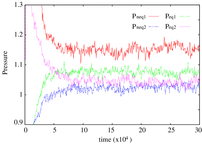
FIG. 2.: The time evolution of pressures in MD simulation where $P_{neq1}$ and $P_{eq1}$ are the result of the simulation for $T_{1}/T_{0}=4$, and $P_{neq2}$ and $P_{eq2}$ are the result for $T_{1}/T_{0}=1/4$.

In Fig.2, the suffices 1 and 2 in the figure correspond to the cases of $T_{1}/T_{0}=4$ and $T_{1}/T_{0}=1/4$. Our result is contrast to those of both SST[9] and the calculation by Kim and Hayakawa[10]. Here, the osmosis $\Delta P$ depends on the gradient of temperature in which $\Delta P$ becomes positive for $T_{1}/T_{0}=4$ and $\Delta P$ becomes negative for $T_{1}/T_{0}=1/4$. This simulation suggests that both SST and the calculation by Kim and Hayakawa cannot be used for Knudsen effect in physical situations.

There are two possibilities to have linear dependence of the osmosis $\Delta P$ on the temperature gradient: (i) Knudsen’s layer effect is important on the thermal wall, and (ii) the assumption of small Knudsen number is violated. As a result of finiteness of Knudsen number which is around 1/50-1/100, the temperature at the place deviated from the hole by the mean-free path is significantly different from the temperature at the hole. We believe that the second possibility plays a dominant role, because the gap of the pressure is enhanced when the nonequilibrium cell has higher temperature, i.e. larger mean-free path $l_{neq}=21.40d$ than that for low temperature nonequilibrium cell $l_{neq}=11.24d$. The details of MD simulation will be reported elsewhere.

V Conclusion

In conclusion, we have explained our recent finding of a new explicit solution of Boltzmann equation under the steady heat conduction. We apply the solution to examine the validity of SST and information theory, and find that both of them are not appropriate as they are. We also discuss the stability of the steady solution we have obtained, and confirmed stability at least for the case of no systematic flow. Through MD simulation of Knudsen effect under the heat conduction, we have obtained the result that $\Delta P$ depends on the direction of the temperature gradient. This indicates that our naive application of the steady solution of Boltzmann equation to Knudsen effect is not accurate. This also suggests that the basic assumption of SST cannot be valid if the influence of physical wall exists.

Acknowledgment: The authors wish to thank M. Fushiki for fruitful discussion and for his sending us the unpublished result of his simulation. This work is partially supported by the Grant-in-Aid of Ministry of Education, Culture, Sports, Science and Technology(MEXT), Japan (Grant No. 15540393) and the Grant-in-Aid for the 21st century COE ’Center for Diversity and Universality in Physics’ from MEXT, Japan.

TABLE I.: The number constants $b_{0r}$ in eq.(16)

$r$	$b_{0r}$	$b_{1r}$	$b_{2r}$
$0$	-	-	$-3.320\times 10^{-2}$
$1$	-	$1.025$	$-1.276\times 10^{-1}$
$2$	$4.380\times 10^{-1}$	$4.892\times 10^{-3}$	$6.414\times 10^{-2}$
$3$	$-5.429\times 10^{-2}$	$3.715\times 10^{-3}$	$5.521\times 10^{-3}$
$4$	$-4.098\times 10^{-3}$	$2.922\times 10^{-4}$	$4.214\times 10^{-3}$
$5$	$-3.184\times 10^{-4}$	$2.187\times 10^{-5}$	3.106$\times 10^{-5}$
$6$	$-2.087\times 10^{-5}$	$1.492\times 10^{-6}$	$1.861\times 10^{-6}$
$7$	-	$8.322\times 10^{-8}$	-

REFERENCES

- [1] S. Chapman and T. G. Cowling, The Mathematical Theory of Non-Uniform Gases , Third Edition (Cambridge University Press, 1970).
- [2] P. Résibois and M. de Leener, Classical Kinetic Theory of Fluids (John Wiley Sons, New York, 1977).
- [3] C. Cercignani, Mathematical Methods in Kinetic Theory(Plenum Press, New York, 1990).
- [4] D. Burnett, The Distribution of Molecular Velocities and the Mean Motion in a Non-Uniform Gas, Proc. Lond. Math. Soc. 1935, 40 (Nov.15), 382-435.
- [5] A. V. Bobylev, The Chapman-Enskog and Grad Method for solving Boltzmann equation, Sov. Phys. Dokl. 1982, 27, 29.
- [6] H. Struchtrup and M. Torrihon, Regularization of Grad’s 13 moment equation: Derivation and linear analysis, Phys. Fluids, 2003, 15 (9), 2668-2680.
- [7] H. Grad, On the kinetic theory of rarefied gas, Commun. Pure Appl. Math. 1949, 2 331-407.
- [8] J. Casas-Várquez and D. Jou, Temperature in non-equilibrium states: a review of open problems and current proporsal , Rep. Prog. Phys. 2003, 66, 1937-2023.
- [9] S. Sasa and H. Tasaki, Steady state thermodynamics, cond-mat/0411052, 2004. See also their previous version in cond-mat/0108365.
- [10] Kim Hyeon-Deuk and H. Hayakawa, Kinetic Theory of a Dilute Gas System under Steady Heat Conduction J. Phys. Soc. Jpn. 2003 , 72 (8), 1904-1916.
- [11] M. Fushiki, private communications. (and his unpublished result).
- [12] Kim Hyeon-Deuk and H. Hayakawa, Test of information theory on the Boltzmann equation J. Phys. Soc. Jpn. 2003 72, (10), 2473-2476.
- [13] Kim Hyeon-Deuk and H. Hayakawa, Contributions of steady heat conduction to the rate of chemical reaction, Chem. Phys. Lett. 2003, 372, (Nos.3-4) 314-319.
- [14] Kim Hyeon-Deuk, in preparation.
- [15] E. M. Lifshitz and Pitaevski, Physical Kinetics(Pergamon, Oxford, 1981).