Photoemission spectra of many-polaron systems

Abstract

The cross over from low to high carrier densities in a many-polaron system is studied in the framework of the one-dimensional spinless Holstein model, using unbiased numerical methods. Combining a novel quantum Monte Carlo approach and exact diagonalization, accurate results for the single-particle spectrum and the electronic kinetic energy on fairly large systems are obtained. A detailed investigation of the quality of the Monte Carlo data is presented. In the physically most important adiabatic intermediate electron-phonon coupling regime, for which no analytical results are available, we observe a dissociation of polarons with increasing band filling, leading to normal metallic behavior, while for parameters favoring small polarons, no such density-driven changes occur. The present work points towards the inadequacy of single-polaron theories for a number of polaronic materials such as the manganites.

I Introduction

In recent years, it has become widely accepted that electron-phonon (EP) interaction plays a crucial role in systems with strong electronic correlations, such as high-temperature superconducting cupratesBar-Yam et al. (1992) or colossal magnetoresistive manganites.Edwards (2002) A large amount of the available data on optical and transport properties has been interpreted in terms of polaronic states. In view of the complex underlying physics, however, the application of single-polaron theories seems to be problematic. On the other hand, a reliable theory of strongly coupled EP systems with finite carrier densities is not available yet. While limiting cases, such as weak coupling or large phonon frequencies—compared to the electronic bandwidth—can to some degree be described theoretically, especially the adiabatic regime of small phonon frequencies at intermediate-to-strong EP coupling constitutes a long-standing, open problem. Since analytical results can only be obtained at the expense of uncontrolled approximations, progress toward an understanding of many-polaron systems requires unbiased numerical methods. Owing to the availability of high performance computers, the latter can yield insight into the properties of basic microscopic models such as the spinless Holstein model considered here. Nevertheless, apart from work on the half-filled band case, where the physics is dominated by a cross over from a Luttinger liquid to a Peierls state, the many-polaron problem has received little attention in the past.

Motivated by this situation, in the present work, we address the important issue of the effect of carrier density on the character of the quasiparticles of the system. While for very strong couplings no significant changes are expected due to the existence of rather independent small (self-trapped) polarons with negligible residual interaction, a density-driven cross over from a state with large polarons to a metal with weakly dressed electrons may occur in the intermediate coupling regime. This problem has recently been investigated experimentally in terms of optical measurements on $\mathrm{La_{2/3}(Sr/Ca)_{1/3}MnO_{3}}$ films.Hartinger et al. (2004, unpublished) While small polarons have been identified as the charge carriers in the low-temperature metallic phase of the Ca doped system, the weaker electron-lattice coupling in the Sr doped system gives rise to large-polaron-like behavior of the optical conductivity. The effect of the finite carrier density on such extended polaronic quasiparticles has been analyzedHartinger et al. (2004, unpublished) using a recently developed weak-coupling theory.Tempere and Devreese (2001)

For the case of the Holstein model, the abovementioned density-driven transition from small to large polarons and finally to weakly EP-dressed electrons is expected to be possible only in one dimension (1D), where large polarons extending over more than one lattice site exist at weak coupling. Existing work indicates that in higher dimensions, the electrons remain quasifree at weak coupling, and become self-trapped above a critical value of the EP coupling strength.De Raedt and Lagendijk (1982, 1983); Kabanov and Mashtakov (1993); Fehske et al. (1995) By contrast, approximate variational calculations suggest that large polarons may also exist in $D>1$.Romero et al. (1999); Cataudella et al. (1999, 2001) The situation is different for Fröhlich-type modelsFröhlich (1954); Alexandrov and Kornilovitch (1999) with long-range EP interaction, in which large polaron states exist even for strong coupling and in higher dimensions.

Here, we make use of quantum Monte Carlo (QMC) and exact diagonalization (ED) methods, and calculate the photoemission spectra for finite clusters at zero and finite temperature. Due to the limitations of existing algorithms, we develop a new grand-canonical QMC approach which is free of autocorrelations and therefore enables us to study small phonon frequencies and low temperatures.

The organization of this paper is as follows. In Sec. II, we present the model and discuss previous work, while Sec. III contains details about the methods we employed. Section IV gives a discussion of our numerical data, and finally, we conclude in Sec. V. The new QMC technique is described in the Appendix.

II Model

The spinless Holstein model is defined by the Hamiltonian

$$H=-t\sum_{\langle i,j\rangle}c^{\dagger}_{i}c^{\phantom{{\dagger}}}_{j}+\omega_{0}\sum_{i}b^{\dagger}_{i}b^{\phantom{{\dagger}}}_{i}-g\omega_{0}\sum_{i}\hat{n}_{i}(b^{\dagger}_{i}+b^{\phantom{{\dagger}}}_{i})\,,$$ (1)

where $c^{\dagger}_{i}$ ($c^{\phantom{{\dagger}}}_{i}$) creates (annihilates) a spinless fermion at lattice site $i$, $b^{\dagger}_{i}$ ($b^{\phantom{{\dagger}}}_{i}$) creates (annihilates) a phonon of energy $\omega_{0}$ ($\hbar=1$) at site $i$, and $\hat{n}_{i}=c^{\dagger}_{i}c^{\phantom{{\dagger}}}_{i}$. While the first term describes hopping processes between neighboring lattice sites $\langle i,j\rangle$, the second term corresponds to the elastic and kinetic energy of the phonons. Finally, the last term in Eq. (1) represents a local coupling of the lattice displacement to the electron occupation $n_{i}=0,\,1$.

The parameters of the model are the hopping integral $t$, the phonon energy $\omega_{0}$, and the coupling constant $g$. The latter is related to the polaron binding energy $E_{\text{P}}$ via $g=\sqrt{E_{\text{P}}/\omega_{0}}$. By defining the dimensionless quantities $\lambda=E_{\text{P}}/2t\text{D}$, and $\overline{\omega}_{0}=\omega_{0}/t$, we are left with two independent parameters. In the sequel, we express all energies in units of $t$. The lattice constant is taken to be unity, and periodic boundary conditions are applied.

The Holstein Hamiltonian (1) represents a generic model for a many-polaron system. Due to the restriction to spinless fermions, on-site bipolaron formation is suppressed.Bonča et al. (2000)

Quantum fluctuations of the lattice enable the electrons to hop even in the strong-coupling regime, while in models with classical phonons translation symmetry is broken, so that no itinerant polaron states exist. Along this line, the half-filled spinless Holstein model has been studied in one dimension using QMC,Hirsch and Fradkin (1982, 1983); McKenzie et al. (1996) ED,Weiße and Fehske (1998) DMRGBursill et al. (1998) and variational methods.Zheng et al. (1989); Feinberg et al. (1990); Zheng and Avignon (1998); Wang et al. (2000); Perroni et al. (2003) Similar to the spinfull model at half filling, the spinless model with one electron per two lattice sites displays a quantum phase transition from a metallic state to a Peierls insulating state with charge-density-wave (CDW) order at $T=0$. While the insulating CDW state of the spinless model is stable for any $\lambda>0$ in the adiabatic limit $\overline{\omega}_{0}=0$, it can be destroyed by quantum phonon fluctuations for $\overline{\omega}_{0}>0$.Bursill et al. (1998) Capone et al. Capone et al. (1999) used ED to study the cross over from a single polaron to a many-electron system away from half filling. Although their work is actually for the Holstein-Hubbard model, results are very similar to the spinless Holstein model in the limit of large $U$ considered in Ref. Capone et al., 1999. The authors found that the critical coupling for polaron formation is unaffected by the electron density in the antiadiabatic regime. Finally, we would like to point out previous analytical efforts to take into account squeezing and correlation effects in many-polaron systems.Zheng et al. (1989); Feinberg et al. (1990); Fehske et al. (1994)

III Methods

In this work we use QMC, and ED in combination with the kernel polynomial method (KPM), to calculate, in particular, single-particle spectra. These two approaches are characterized by different advantages and shortcomings. ED in the form used here yields exact spectra at $T=0$ with extremely high energy resolution. However, even for relatively small clusters of ten sites—the size used here—this method requires parallel supercomputers to handle the enormous Hilbert space (matrix dimension $\approx 10^{7}$ – $10^{10}$). Consequently, the momentum resolution, determined by the cluster size, is rather crude.

In contrast, the grand-canonical QMC simulations can be performed on personal computers, and for larger clusters. The drawback is that (a) the method is limited to finite temperatures, and (b) the calculation of spectral properties requires the analytic continuation from imaginary time to real frequencies, which is an ill-conditioned problem. Therefore, regularization techniques such as the maximum entropy method (MEM) used here have to be applied, which offer only limited energy resolution and may introduce uncontrolled errors. For this reason, we will also present a direct comparison of ED and QMC results.

III.1 Quantum Monte Carlo

In applying existing QMC methods for the Holstein model to the parameter regime considered here, one faces extremely long autocorrelations times, as well as large statistical errors.Hohenadler et al. (2004) This makes it very difficult to obtain accurate results for spectral properties, due to the use of the MEM. To overcome these problems, the algorithm presented in the Appendix is based on the canonical Lang-Firsov transformation.Lang and Firsov (1962) The latter explicitly contains the shift of the lattice equilibrium position in the presence of an electron, which is favorable for the QMC simulations. Moreover, the absence of a direct coupling between the electron density and the lattice displacements in the transformed Hamiltonian (5) permits exact, uncorrelated sampling of the phonon degrees of freedom (momenta) in terms of principal components.

Here we have mainly used a value of $\beta t=8$ for the inverse temperature $\beta=1/k_{\text{B}}T$. For the critical parameters studied below, accurate simulations at even lower temperatures become very demanding due to a minus-sign problem (Sec. A.3). Nevertheless, we shall present results for the density of states at $\beta t=10$ and half filling but for a reduced cluster size. Note that already for $\beta t=8$ we have $k_{\text{B}}T/t=0.125<\overline{\omega}_{0}$ for the values $\overline{\omega}_{0}\geq 0.4$ used in the sequel, so that direct thermal excitation of phonons is expected to be rather unimportant.

For the Trotter decomposition, we chose $\Delta\tau=0.05$ (see Appendix) for static observables. Owing to the larger numerical effort associated with the calculation of dynamical properties, for the latter we use $\Delta\tau=0.1$—the larger error being small compared to the uncertainties introduced by the MEM inversion. The Trotter error in the Holstein model becomes important mainly for large phonon frequencies and very strong EP interaction.Kornilovitch (1997); Hohenadler et al. (2004) Since we do not consider this regime here, the abovementioned values of $\Delta\tau$ yield satisfactorily small systematic errors.

Away from half filling, the electron density has to be adjusted to the values of interest by varying the chemical potential $\mu$. Due to the computational effort associated with this trial-and-error procedure, the actual band filling $n^{\prime}$, say, is usually only very close to a desired value, e.g., $n=0.4$, but not exactly the same. Furthermore, within the QMC simulations, the filling can only be determined up to a statistical error $\Delta n^{\prime}$, similar to other observables. For the results presented here, the relative deviation $(n-n^{\prime})/n$ of the actual value in the QMC simulations from the value $n$ reported is always smaller than $5\times 10^{-3}$. The same is true for the relative statistical error $\Delta n^{\prime}/n$.

To perform the continuation of the one-electron Green function from imaginary time to real frequencies, we use the MEM (for a review see, e.g., Ref. Jarrell and Gubernatis, 1996). The algorithm employed here incorporates an improved evidence approximation,von der Linden et al. (1999) which is less susceptible to overfitting—resulting in peaks whose position, weights and even existence are not clear—than the conventional evidence approximation.Jarrell and Gubernatis (1996) On the other hand, groups of narrowly spaced peaks are represented by an envelope if the accuracy of the QMC data is not sufficient.

The proposal of an alternative evidence approximation—leading in general to stronger regularization and, consequently, lower energy resolution than the conventional approximation—may not seem advantageous at first. However, considering the great variety of different spectra compatible with the QMC data within the error bars due to the extremely ill-conditioned analytical continuation problem, we argue that it rather corresponds to choosing the “most uninformative” solution in the spirit of the maximum entropy principle. In fact, we found that the alternative evidence approximation yields much more consistent results than the “classic” evidence approximationJarrell and Gubernatis (1996) when we subjected artificial test data to different noise while keeping the signal-to-noise ratio fixed. A detailed comparison of different regularization schemes available will be presented elsewhere.

In order to scrutinize the resulting spectra, the following test has been performed. Following the idea of Silver et al.,Silver et al. (1990) the results from the MEM applied to the original QMC data $G(k,\tau)$ have been taken as an “exact” spectral function $A(k,\omega)$, from which mock data $\tilde{G}(k,\tau)$ for the imaginary-time Green function has been created by using Eq. (22) and adding Gaussian random noise of absolute size $10^{-3}$ – $10^{-4}$, comparable to the statistical errors of the QMC results. Again using the MEM to invert these data, the thereby obtained spectral function $\tilde{A}(k,\omega)$ allows to check the stability of the MEM result $A(k,\omega)$ with respect to statistical errors. We find that the features in our results for $A(k,\omega)$ remain stable if $G(k,\omega)$ varies within the statistical errors, so that the data presented below are satisfactorily reliable apart from the aforementioned broadening and the limited energy resolution.

While our method is completely free of autocorrelations between subsequent phonon configurations, results for the imaginary-time Green function at different times are usually not statistically independent.von der Linden et al. (1996) However, in the present case, owing to the exact sampling and the large number of measurements, these correlations are very small and have been neglected since they have negligible influence on the results. An additional, stringent test of the QMC results consists of a comparison to ED data which will be presented in Sec. IV.2.

Finally, we note that all QMC simulations have been run on personal computers (e.g., Intel XEON 2600 MHz), with CPU times varying between several hours and a couple of days.

III.2 Exact diagonalization

The combination of ED and KPM has been described in detail in Ref. Bäuml et al., 1998. In this work, we are mainly interested in the single-particle spectral functions

$$\begin{split}A^{+}(k,\omega)=\sum_{l}|&\langle\Psi_{l,k}^{(N_{\text{e}}+1)}|c^{\dagger}_{k-q}|\Psi_{0,q}^{(N_{\text{e}})}\rangle|^{2}\,\\ &\times\delta[\omega-(E_{l,k}^{(N_{\text{e}}+1)}-E_{0,q}^{(N_{\text{e}})})]\,,\end{split}$$

$$\begin{split}A^{-}(k,\omega)=\sum_{l}|&\langle\Psi_{l,k}^{(N_{\text{e}}-1)}|c^{\phantom{{\dagger}}}_{q-k}|\Psi_{0,q}^{(N_{\text{e}})}\rangle|^{2}\,\\ &\times\delta[\omega+(E_{l,k}^{(N_{\text{e}}-1)}-E_{0,q}^{(N_{\text{e}})})]\,,\end{split}$$ (2)

where $|\Psi^{(N_{\text{e}})}_{l,k}\rangle$ denotes the $l$th eigenstate with $N_{\text{e}}$ electrons, momentum $k$ and energy $E_{l,k}^{(N_{\text{e}})}$. The cluster size has been fixed at $N=10$, with as many as 15 dynamical phonons and resulting truncation errors $<10^{-6}$ for the ground-state energy.Bäuml et al. (1998) Additionally, the convergence with the number of phonons has been monitored by means of the phonon distribution function.Bäuml et al. (1998) It is important to point out that such a small number of dynamical phonons only yields accurate results for the parameters considered here if the symmetric phonon mode with $q=0$ is separated from the Hamiltonian analytically before the diagonalization.Robin (1997); Sykora et al. (2005) In the present case, this phonon mode—corresponding to a homogeneous shift of the oscillator equilibrium positions—together with that for $q=\pi$ represents the dominant contribution to phonon excitations, so that the separation is very efficient at reducing the computational effort. The largest matrix dimension in the present calculations was about $3\times 10^{8}$, running on six compute nodes of a Hitachi SR8000-F1. The energy resolution of the KPM spectral function with 512 moments has been enhanced by a factor of 8 by the MEM,Bäuml et al. (1998) resulting in a significantly better resolution compared to, e.g., the spectral decoding method. We would like to point out that in contrast to the case of QMC, the ED data to which the MEM is applied does not have a statistical error.

IV Results

It is long known that within the Holstein model (1), a single electron undergoes a cross over to a small polaron at a critical value of the EP coupling.De Raedt and Lagendijk (1982) The important question to be addressed here is what happens if the density of electrons (or polarons) is increased. We do not expect significant changes in the strong-coupling regime due to the rather “localized” nature of the small polaron state. On the contrary, for intermediate EP interaction and $\overline{\omega}_{0}<1$, each electron is surrounded by a phonon cloud extending over several lattice sites. Now, at larger densities, a substantial overlap of the single-particle wavefunctions occurs, leading to a dissociation of the individual polarons and finally to a restructuring of the whole many-particle ground state. Furthermore, it has been shown that squeezing effects reduce the polaronic band-narrowing in the many-electron case,Fehske et al. (1994) thereby favoring such a scenario. Since within the Holstein model, a large polaron state is expected to be stable in 1D, we will only consider this case in the sequel.

In view of the situation in most polaronic materials, we mainly consider the adiabatic regime, taking $\overline{\omega}_{0}=0.4$. To illustrate the important differences between $\overline{\omega}_{0}\ll 1$ and $\overline{\omega}_{0}\gg 1$, however, some results for the antiadiabatic value $\overline{\omega}_{0}=4$ will also be shown.

IV.1 Limiting cases

As we shall see below, the spectra in the intermediate coupling region turn out to have a fairly complex structure. It is therefore helpful to begin with the limiting cases of weak and strong EP coupling.

IV.1.1 Weak coupling

For weak coupling $\lambda=0.1$, the sign problem is not severe (Sec. A.3) and the QMC simulations can easily be performed for large lattices with $N=32$, thereby making the dispersion of quasiparticle features well visible. As indicated in Eq. (22), the MEM inversion yields $A(k,\omega-\mu)$, where $\mu$ denotes the chemical potential.

Figure 1: One-electron spectral function $A(k,\omega-\mu)$ from QMC for different band fillings $n$, $N=32$, $\beta t=8$, $\overline{\omega}_{0}=0.4$, and weak coupling $\lambda=0.1$.

Figure 1 shows the evolution of the one-electron spectral function $A(k,\omega-\mu)$ with increasing electron density $n$. At first sight, we see that the spectra bear a close resemblance to the free-electron case, i.e., there is a strongly dispersive band running from $-2t$ to $2t$. The latter can be attributed to weakly dressed electrons with an effective mass similar to the noninteracting case. As expected, the height (width) of the peaks increases (decreases) significantly in the vicinity of the Fermi momentum $k_{\text{F}}$, which is determined by the crossing of the band with the chemical potential.

Figure 2: One-electron density of states $\rho(\omega-\mu)$ from QMC for different band fillings $n$, $N=32$, $\beta t=8$, $\overline{\omega}_{0}=0.4$ and $\lambda=0.1$.

Since the peaks in Fig. 1 are generally very sharp, it is important to check the results from the inversion with the MEM. By computing the approximate number of electrons corresponding to the fillings $n=0.1$ – 0.4 of the 32-site system, we can roughly determine $k_{\text{F}}$. Although the nonzero EP interaction will affect the band dispersion $E(k)$, the weak coupling considered here justifies the use of a rigid band approximation, as reflected in the free-particle character of the spectra in Fig. 1.

For $n=0.1$, i.e., about three electrons for $N=32$, the Fermi momentum is expected to lie between $k=\pi/16$ and $k=\pi/8$, corresponding to the second and third curve from the top in Fig. 1(a). In fact, we see that the largest peaks are those for $k=\pi/16$ and $\pi/8$, having almost the same height. Above and below these momenta, the peaks are noticeably smaller. A similar analysis carried out for the other fillings in Figs. 1(b) – (d) also shows a very good agreement between the location of the highest peaks and the estimated values of $k_{\text{F}}$.

Finally, we would like to point out that the apparent absence of any phonon signatures in Fig. 1 is not a defect of the MEM, but results form the large scale of the $z$-axis chosen. As a consequence, the peaks running close to the bare band dominate the spectra and suppress any small phonon peaks present. If we enlarge the resolution, for all densities $n=0.1$ – 0.4, we observe the band flatteningStephan (1996); Wellein and Fehske (1997); Hohenadler et al. (2003) at large wavevectors which originates from the intersection of the approximately free-electron dispersion with the optical phonon energy occurring at $\omega-\mu=\omega_{0}$.

To complete our discussion of the weak-coupling regime, we show in Fig. 2 the one-electron density of states (DOS) $\rho(\omega-\mu)$ given by Eq. (25). Clearly, for small $n$, there is a peak with large spectral weight at the Fermi level. In contrast, for large $n$, the tendency toward formation of a Peierls– (band–) insulating state at $n=0.5$ suppresses the DOS at the Fermi level, although we are well below the critical value of $\lambda$ at which the cross over to the insulating state takes place at $T=0$.Bursill et al. (1998) The additional small features separated from $\mu$ by the bare phonon energy $\omega_{0}$ will be discussed in the intermediate coupling case below.

IV.1.2 Strong coupling

Figure 3: One-electron spectral function $A(k,\omega-\mu)$ from QMC for different band fillings $n$, $N=32$, $\beta t=8$, $\overline{\omega}_{0}=0.4$, and strong coupling $\lambda=2.0$.

We now turn our attention to the opposite limit of the spinless Holstein model, namely the case of strong EP coupling $\lambda=2$. While calculations with many other numerical methods such as, e.g., standard grand-canonical QMC or ED, become very difficult in this regime, the QMC approach used here yields quite accurate results even for large systems. The improved statistics in the strong-coupling regime is also reflected in the dependence of the average sign on $\lambda$ (cf. the discussion of Fig. 12 in the Appendix). As before, we study the dependence of the spectral function on the band filling, again for $N=32$. The results are depicted in Fig. 3.

In the low-density regime $n=0.1$ [Fig. 3(a)], we expect the well-known almost flat polaron band having exponentially reduced spectral weight (given by $e^{-g^{2}}$ in the single-electron, strong-coupling limit) which, nevertheless, can give rise to coherent transport at $T=0$. Unfortunately, the QMC/MEM has difficulties resolving such extremely weak signatures, especially at larger $n$, where the statistical errors are more noticeable, and for temperatures such that the thermal energy is comparable to the polaron band width. Therefore the polaron band can hardly be resolved in Figs. 3(a) or (b), and is not even detectable in Figs. 3(c) and (d). However, if we consider a density $n=0.05$, corresponding to a single electron on a cluster with $N=20$, at a lower temperature $\beta t=10$, the QMC results do indeed give a polaron band around $\mu$ (Fig. 4). Due to the sign problem, similar calculations for $n>0.1$ would be very demanding.

Besides, the spectrum consists of two incoherent features located above and below the chemical potential, which reflect the phonon-mediated transitions to high-energy electron states. Here, the maximum of the photoemission spectra ($\omega-\mu>0$) follows a tight-binding cosine dispersion. The incoherent part of the spectra is broadened according to the phonon distributions. We would like to mention that the spectrum of a single polaron at strong EP coupling has been studied analytically by Alexandrov and Ranninger.Alexandrov and Ranninger (1992)

Figure 4: Dispersion of the polaron band in $A(k,\omega-\mu)$ for $n=0.05$, $N=20$ and $\beta t=10$ (drawn to a larger scale as compared to Fig. 3). All other parameters as in Fig. 3.

With increasing band filling [see panels (b) and (c)], the chemical potential is shifted to lower energies $\propto E_{\text{P}}n$, but is expected to be still located in a narrow band with little spectral weight. Regardless of the aforementioned shortcomings, the QMC results provide a clear picture of the physics. There exists a finite gap to the photoemission (inverse photoemission) parts of the spectrum, so that the system typifies as a polaronic metal. We shall see below that a completely different behavior is observed at intermediate coupling. Notice that the incoherent inverse photoemission (photoemission) signatures are more pronounced at small (large) wavevectors.

Finally, for $n=0.4$ [Fig. 3(d)], the incoherent features lie rather close to the Fermi level, thus being accessible by low-energy excitations. Now, the photoemission spectrum for $k<\pi/2$ becomes almost symmetric to the inverse photoemission spectrum for $k>\pi/2$ and already reveals the gapped structure which occurs at $n=0.5$ due to the CDW-formation accompanied by a Peierls distortion.

As in the weak-coupling case discussed above, the properties of the system also manifest itself in the DOS, shown in Fig. 5. Owing to the strong EP interaction, the spectral weight at the chemical potential is exponentially small for all fillings $n$.

At half filling, the DOS exhibits particle-hole symmetry, and the system can be described as a Peierls insulator, consisting of a polaronic superlattice. In contrast to the weak-coupling case, the ground state is characterized as a polaronic insulator rather than a band insulator. Moreover, here the gap at the Fermi level persists even at the finite temperature used in the simulation, while for $\lambda=0.1$ and $n=0.5$ the insulating state found at $T=0$ is destroyed by thermal fluctuations (Fig. 2). Note that, owing to the sign problem, the result for $n=0.5$ in Fig. 5 is for a reduced cluster size $N=20$. However, in the strong-coupling regime considered here, finite-size effects are expected to be very small.

Figure 5: One-electron density of states $\rho(\omega-\mu)$ from QMC for different band fillings $n$ and cluster sizes $N$, $\beta t=8$, $\overline{\omega}_{0}=0.4$ and $\lambda=2.0$.

Figure 6: One-electron spectral function $A(k,\omega-\mu)$ from QMC for different band fillings $n$ and cluster sizes $N$, $\beta t=8$, $\overline{\omega}_{0}=0.4$, and intermediate coupling $\lambda=1.0$.

IV.2 Intermediate coupling

As discussed in the introduction, a cross over from a polaronic state to a system with weakly dressed electrons can be expected in the intermediate coupling regime. Here we choose $\lambda=1$, which corresponds to the critical value for the small-polaron cross over in the one-electron problem (cf., e.g., Fig. 5 in Ref. Hohenadler et al., 2004).

IV.2.1 Quantum Monte Carlo

We first discuss the QMC results. Owing to the sign problem, which is particularly noticeable for $\lambda=1$ (see Appendix), we have to decrease the system size as we increase the electron density $n$.

Figure 6 shows the spectral function for $\lambda=1$ and increasing band filling. Owing to the overlap of large polarons in the intermediate coupling regime, we start with the very low density case $n=0.05$ [Fig. 6(a)]. Compared to the behavior for $\lambda=2$ [Fig. 3(a)], we notice that the polaron band now lies much closer to the incoherent features, and that there is a mixing of these two parts of the spectrum at small values of $k$. Nevertheless, the almost flat polaron band is well visible for large $k$.

With increasing density, the polaron band merges with the incoherent peaks at higher energies. This is the above-anticipated density-driven cross over from a polaronic to a (diffusive) metallic state, with the main band crossing the Fermi level. At $n=0.4$, we find a band with large effective width ranging from $\omega\approx-4t$ to $\omega\approx 2t$. A more detailed discussion of the spectral function will be given below when we present ED results.

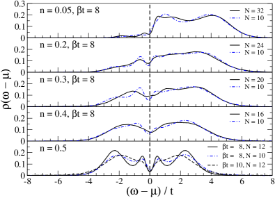
Figure 7: (color online) One-electron density of states $\rho(\omega-\mu)$ from QMC for different band fillings $n$, cluster sizes $N$ and inverse temperatures $\beta$. Here $\overline{\omega}_{0}=0.4$ and $\lambda=1.0$.

Further information about the density dependence can be obtained from the one-electron DOS. The latter is presented in Fig. 7 for different fillings $n=0.05$ – 0.5. As in Fig. 6, the cluster size is reduced with increasing $n$ in order to cope with the sign problem. To illustrate the rather small influence of finite-size effects, Fig. 7 also contains results for $N=10$.

For low density $n=0.05$, the DOS in Fig. 7 lies in between the results for weak and strong coupling discussed above. Although the spectral weight at the chemical potential is strongly reduced compared to $\lambda=0.1$, $\rho(0)$ is still significantly larger than for $\lambda=2.0$.

When the density is increased to $n=0.2$, the DOS at the chemical potential increases, as a result of the dissociation of the polarons. As we increase $n$ further, a pseudogap begins to form at $\mu$, which is a precursor of the CDW gap at half filling and zero temperature.

Finally, in the case of half filling $n=0.5$, the DOS has become symmetric with respect to $\mu$. There are broad features located either side of the chemical potential, which take on maxima close to $\omega-\mu=\pm E_{\text{P}}$. However, apart from the strong-coupling case, where the single-polaron binding energy is still a relevant energy scale, the position of these peaks is rather determined by the energy of the upper and lower bands, split by the formation of a Peierls state. The gap of size $\sim\lambda$ expected for the insulating charge-ordered state at $T=0$ is partially filled in due to the finite temperature considered here.

Furthermore, we find additional, much smaller features roughly separated from $\mu$ by the bare phonon frequency $\omega_{0}$, whose height decreases with decreasing temperature, as revealed by the results for $\beta t=10$ (Fig. 7). These peaks—not present at $T=0$ (see Ref. Sykora et al., 2005)—arise from thermally activated transitions to states with additional phonons excited, and are also visible in Figs. 2 and 5. While for weak coupling [$E_{\text{P}}=0.2$, $\lambda=0.1$, Fig. 2], the maximum of these features is almost exactly located at $|\omega-\mu|=\omega_{0}$, it moves to $|\omega-\mu|\approx 1.25\omega_{0}$ for intermediate coupling [$Ep=2$, $\lambda=1$, Fig. 7], and finally to $|\omega-\mu|\approx 2.5\omega_{0}$ for strong coupling [$E_{\text{P}}=4$, $\lambda=2$, Fig. 5]. Although the exact positions of the peaks are subject to uncertainties due to the MEM, this reflects the shift of the maximum in the phonon distribution function with increasing coupling. The MEM yields an envelope of the multiple peaks separated by $\omega_{0}$.

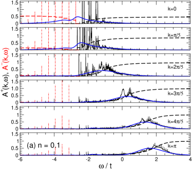
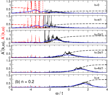
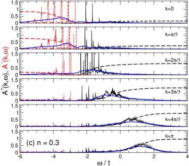
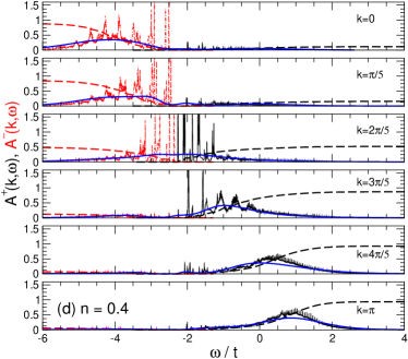
Figure 8: (color online) One-electron spectral functions $A^{-}(k,\omega)$ (red dot-dashed lines) and $A^{+}(k,\omega)$ (black thin solid lines) from ED for different band fillings $n$, $N=10$, $\overline{\omega}_{0}=0.4$, and intermediate coupling $\lambda=1.0$. Also shown are the integrated spectral weights of $A^{-}$ and $A^{+}$ (dashed lines), as well as $A(k,\omega)$ from QMC for $N=10$ and $\beta t=8$ (blue thick solid lines).

At this point, we would like to mention the exact relationKornilovitch (2002)

$$M_{1}(k)=\int_{-\infty}^{\infty}\,d\omega\,\omega\,A(k,\omega)=\varepsilon_{k}-\mu-2E_{\text{P}}n$$ (3)

for the first moment of the one-particle spectral function of the spinless Holstein model, with $\varepsilon_{k}=-2t\cos k$. While the zeroth moment is identical to the normalization of $A(k,\omega)$ for each $k$, $M_{1}(k)$ depends in a nontrivial way on the parameters of the system. In principle, Eq. (3) may be used as a boundary condition in the MEM.White (1991) However, in the present case, we have found that while the normalization is virtually exact for all results shown, the first moment deviates from the exact values. Moreover, the use of the exact values for $M_{1}$ as a condition in the inversion causes the MEM not to converge for some parameters. Additional calculations on small systems reveal that this disagreement results from the finite Trotter error, despite the relatively small value $\Delta\tau=0.1$ used. Away from parameters such that $M_{1}\approx 0$, $M_{1}$ as determined from the MEM spectra deviates from the exact values by maximally 10 – 20 percent. Nevertheless, the peak positions and weights in the spectra shown are fairly accurate, as illustrated by the comparison with ED below. Finally, we would like to point out that calculations of $A(k,\omega)$ for $\Delta\tau<0.1$ become very time-consuming due to the increasing requirement in disk space (see Appendix) and longer simulation times.

Despite the wealth of information contained in the QMC results presented so far, it is obvious that an interpretation of the various excitations is far from being easy. In addition to the finite temperature, the QMC method used here does not allow to separately calculate the photoemission and inverse photoemission parts $A^{-}$ and $A^{+}$, respectively. Moreover, the use of the MEM limits the energy resolution and introduces uncertainties concerning the positions and weights of structures in the spectra. These circumstances make it difficult, e.g., to distinguish between phononic and electronic contributions, especially if $\lambda\approx\overline{\omega}_{0}$. To gain further insight, we therefore supplement the QMC data with ED results.

IV.2.2 Exact diagonalization

In order to overcome the abovementioned limitations of QMC, here we use ED in combination with the KPM, as described in Sec. III.2, to calculate the one-particle spectral functions defined by Eq. (III.2). To test the quality of the QMC spectra, we directly compare the two methods, keeping in mind that the QMC calculations have been performed at a finite temperature, whereas ED yields ground-state results.

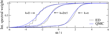
Figure 9: (color online) Comparison of the integrated spectral weight obtained from the QMC and ED data of Fig. 8(a) for three different momenta $k$.

Figure 8 displays the ED results for the same parameters as in Fig. 6, i.e., $\overline{\omega}_{0}=0.4$, $\lambda=1$, and $n=0.1$ – 0.4. Additionally shown are the integrated spectral weights of $A^{-}$ and $A^{+}$ (dashed lines), as well as QMC results for the same system size and $\beta t=8$ (solid thick lines), which have been shifted by $\mu$. The Fermi level lies between the highest-energy peak in $A^{-}$ and the lowest-energy peak in $A^{+}$.

We see from Fig. 8 that the QMC results are compatible with the ED data. Because of the finite temperature and the use of the MEM, QMC, of course, cannot reproduce the sharp ED peaks. To further test the agreement between the two methods, we compare in Fig. 9 the integrated spectral weight of the data shown in Fig. 8(a), and find a very satisfactory accord. Moreover, this agreement becomes even better for larger densities $n$, for which the sharp peaks in the ED data evolve into bands [see Fig. 8(b) – (d)].

In addition to the possibility of distinguishing between $A^{+}$ and $A^{-}$—crucial for an identification of polaron bands at intermediate coupling—the higher energy resolution of ED also allows to resolve signatures of phonon excitations.

Starting with the case $n=0.1$ [Fig. 8(a)], we notice that there is a polaron band at the Fermi level, excitations to/from which are given by the highest (lowest) peak of $A^{-}$ ($A^{+}$). The photoemission part $A^{-}$ reflects the Poisson-like phonon distribution of the one-electron ground state ($n=0.1$ and $N=10$). The integrated spectral weight gives a measure for the electronic weight of the various poles in the one-electron spectrum. For example, it reveals that the phonon peaks in $A^{-}$ have very little weight. In fact, the integrated weight jumps to a finite value at the first peaks near the Fermi level for $k=0$ and $k=\pi/5$, while it changes very little as one moves further down in energy. For $k>\pi/5$, the small spectral weight contained in $A^{-}$ is continuously distributed among the phonon peaks.

We also observe the well-known flattening of the polaron band at large values of $k$. Similar to the one-electron case,Hohenadler et al. (2003) the low-energy states have mostly electronic character at small $k$, and become mostly phononic at large values of $k$. While this effect is expected to occur in the low-density regime, we find that is persists even for $n=0.4$ [Fig. 8(d)]. Moreover, Fig. 8 reveals that the maximum in the incoherent contribution follows closely the free-electron dispersion for all densities $n=0.1$ – 0.4.

With increasing electron density, the equally spaced peaks in $A^{-}$ broaden significantly, until at $n=0.4$ they have merged to form a broad band. The polaron band is still visible at $n=0.2$ [Fig. 8(b)], but becomes indistinguishable from the incoherent excitations at even larger $n$. Eventually, at $n=0.4$ [Fig. 8(d)], we find an almost symmetric behavior of $A^{+}$ and $A^{-}$ with respect to the Fermi level at $k=2\pi/5$. Compared to the strong-coupling case [Fig. 3(d)], there exist incoherent excitations with almost zero energy. This indicates the metallic character of the system expected for large polaron densities and intermediate EP coupling.

IV.3 Antiadiabatic regime

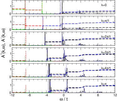
Figure 10: (color online) One-electron spectral functions $A^{-}(k,\omega)$ and $A^{+}(k,\omega)$ from ED for $N=10$, $\overline{\omega}_{0}=4.0$, and $\lambda=2.0$. Here $n=0.1$ ($A^{-}$: red dot-dashed lines, $A^{+}$: black solid lines) and $n=0.3$ ($A^{-}$: green dashed two-dotted lines, $A^{+}$: blue dotted lines). Dashed lines correspond to the integrated spectral weight of $A^{-}(k,\omega)$ and $A^{+}(k,\omega)$, respectively.

Until here, we have only presented results for the adiabatic case $\overline{\omega}_{0}=0.4$. Although the latter is most relevant for strongly correlated materials, it is important to compare the above findings to the antiadiabatic strong-coupling regime. To this end, we chose $\overline{\omega}_{0}=4$ as well as $\lambda=2$. The condition for the formation of a single small polaron in this case, however, is $g\gtrsim 1$, because the phonon frequency is the important energy scale. In contrast, the criterion $\lambda>1$ is purely based on the balance of kinetic and potential energy.Wellein and Fehske (1997); Capone et al. (1997); Ciuchi et al. (1997)

The spectral function for $n=0.1$ and $n=0.3$ is displayed in Fig. 10 for $g=1$, i.e., at the transition point where self-trapping occurs for a single particle. Contrary to the case $\lambda=1$ and $\overline{\omega}_{0}=0.4$ considered above, the absorption features are now separated by the phonon energy $\omega_{0}$, with their width being determined by electronic excitations.

A comparison of the spectral functions for $n=0.1$ and $n=0.3$ in Fig. 10 indicates that there is no density-driven cross over of the system as observed in the adiabatic case. In particular, owing to the large phonon energy, there are no low-energy excitations close to the polaron band, so that the latter remains well separated from the incoherent features even for $n=0.3$. Furthermore, the spectral weight of the polaron band also remains almost unchanged as we increase the density from $n=0.1$ to $n=0.3$. Consequently, almost independent small polarons are formed also at finite electron densities, in accordance with previous findings of Capone et al. Capone et al. (1999) for small systems.

IV.4 Kinetic energy

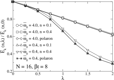
Figure 11: Normalized kinetic energy as a function of EP coupling $\lambda$ for different band fillings $n$ and adiabatic ratios $\overline{\omega}_{0}$. Also shown are the results for a single polaron, obtained with the method of Ref. Hohenadler et al., 2004. Errorbars are smaller than the symbols used and $\Delta\tau=0.05$.

Previously, the electronic kinetic energy has been studied extensively to monitor the polaron and bipolaron cross over in the Holstein model with one and two electrons (see, e.g., Refs. De Raedt and Lagendijk, 1982 and De Raedt and Lagendijk, 1986). Here, at least in the adiabatic regime, polaron formation manifests itself in a drop of the kinetic energy around the critical coupling. In the following, however, we illustrate that the kinetic energy [Eq. (19)] does not reflect the significant changes in the one-particle spectrum we found with increasing density in the intermediate coupling regime (see Sec. IV.2).

To compare different band fillings, we consider the normalized quantity $\overline{E}_{\text{k}}(n,\lambda)/\overline{E}_{\text{k}}(n,0)$, shown in Fig. 11 as a function of EP coupling for different fillings and phonon frequencies, for a fixed system size $N=16$ and $\beta t=8$.

In the adiabatic regime $\overline{\omega}_{0}=0.4$, owing to the overlap of the phonon clouds surrounding the individual quasiparticles, the carriers clearly become more mobile with increasing density, but the change in the kinetic energy is nevertheless surprisingly small. In addition to these two fillings, we have also included in Fig. 11 the result for a single polaron with the same parameters, calculated with the QMC method of Ref. Hohenadler et al., 2004, which is indistinguishable from the result for $n=0.1$.

As expected from the almost identical spectra for $n=0.1$ and 0.3 presented in Sec. IV.3 for the antiadiabatic regime, $\overline{E}_{\text{k}}$ is almost independent of $n$ in this case.

V Conclusions

Strongly correlated electron-phonon systems in dependence on the carrier density have been studied by means of unbiased numerical methods. Using exact diagonalization together with the kernel polynomial method, as well as a novel quantum Monte Carlo approach, we were able to present accurate results for the one-dimensional spinless Holstein model in the most difficult regime of small phonon frequencies and intermediate to strong electron-phonon interaction.

We have calculated the one-particle spectral function, the density of states and the electronic kinetic energy at different band fillings. While exact diagonalization is restricted to relatively small clusters, thereby limiting the momentum resolution of the spectra, quantum Monte Carlo can be used to study larger systems, but yields a lower energy resolution for dynamical quantities. The reliability of the results from the maximum entropy inversion has been scrutinized, and we find a very good agreement between the two methods.

In the adiabatic case, characteristic for, e.g., the manganites, we observe a carrier density-driven cross over from a polaronic state to a metallic system at weak and intermediate electron-phonon coupling. Note that the nature of the quasiparticles is changed in the course of this transition. This points toward an insufficiency of simple single-polaron theories to explain experimental results for polaronic materials. In fact, very similar effects due to carrier interaction have recently been observed experimentally for the manganites.Hartinger et al. (2004, unpublished)

On the contrary, for large phonon frequencies and strong coupling, the individual polarons remain virtually unaffected upon increasing the electron density. Consequently, the system remains polaronic even at large band fillings. Finally, the kinetic energy is shown to be too insensitive in order to reveal the above cross over.

For weak electron-phonon coupling, the system becomes a Peierls or band insulator at half filling, whereas for strong coupling a polaronic insulating state with an exponentially small polaron band at the Fermi level, and a finite gap to the incoherent excitations, prevails for all fillings.

Finally, reliable calculations of the optical conductivity are highly desirable in order to explain the large amount of available experimental data for polaronic materials. Work along this line is in progress.

Appendix A Quantum Monte Carlo

In this Appendix we extend the one-electron QMC algorithm developed in Ref. Hohenadler et al., 2004, henceforth also referred to as I, to the spinless Holstein model with many electrons. We begin by applying the Lang-Firsov transformationLang and Firsov (1962) $\hat{\nu}=\exp(\mathrm{i}\gamma\sum_{j}\hat{n}_{j}\hat{p}_{j})$ with $\gamma^{2}=4\lambda\text{D}/\overline{\omega}_{0}$ to the Hamiltonian (1) in first quantization and with dimensionless phonon variables $\hat{x}$ and $\hat{p}$, which takes the formHohenadler et al. (2004)

$$H=-t\sum_{\langle i,j\rangle}c^{\dagger}_{i}c^{\phantom{{\dagger}}}_{j}+\frac{\omega_{0}}{2}\sum_{i}(\hat{p}^{2}_{i}+\hat{x}^{2}_{i})-\alpha\sum_{i}\hat{n}_{i}\hat{x}_{i}\,.$$ (4)

The coupling constant $\alpha$ is related to that in Eq. (1) by $\alpha=\sqrt{2}g\omega_{0}$. Using the result $\tilde{H}=\hat{\nu}H\hat{\nu}^{\dagger}$ (see I), we define the grand-canonical Hamiltonian

$$\tilde{\mathcal{H}} = \tilde{H}-\mu\sum_{i}\hat{n}_{i}$$ (5)

$$= \underbrace{-t\sum_{\langle i,j\rangle}c^{\dagger}_{i}c^{\phantom{{\dagger}}}_{j}e^{\mathrm{i}\gamma(\hat{p}_{i}-\hat{p}_{j})}}_{\tilde{K}}+\underbrace{\frac{\omega_{0}}{2}\sum_{i}(\hat{p}^{2}_{i}+\hat{x}^{2}_{i})}_{P\equiv P_{p}+P_{x}}$$

$$-\underbrace{(E_{\text{P}}+\mu)\sum_{i}\hat{n}_{i}}_{\tilde{I}}\,,$$

where $\mu$ denotes the chemical potential and $E_{\text{P}}$ is the polaron binding energy.

For the case of a half-filled band, the chemical potential is given by $\mu=-E_{\text{P}}$. Away from $n=0.5$, $\mu$ has to be adjusted accordingly to yield the right density of electrons $n$.

We would like to point out that in the spinfull case, the transformed Hamiltonian would contain an attractive Hubbard term. For the determinant QMC method to be applicable, the latter has to be decoupled using auxiliary fields.von der Linden (1992) In contrast, for the spinless model considered here, the algorithm is almost identical to the one-electron case. The following derivation assumes a hypercubic lattice in D dimensions, consisting of $N^{\text{D}}$ sites.

A.1 Partition function

We use the Suzuki-Trotter decompositionvon der Linden (1992)

$$e^{-\beta\tilde{\mathcal{H}}}\approx\left(e^{-\Delta\tau\tilde{K}}e^{-\Delta\tau P_{\text{p}}}e^{-\Delta\tau P_{\text{x}}}e^{-\Delta\tau\tilde{I}}\right)^{L}\,,$$ (6)

with $\Delta\tau=\beta/L$. The trace appearing in the partition function $\mathcal{Z}=\text{Tr}\,e^{-\beta\tilde{\mathcal{H}}}$ can be split up into a bosonic and a fermionic component leading to

$$\mathcal{Z}_{L}= \text{Tr}\,_{\text{f}}\int\,dp_{1}dp_{2}\cdots dp_{L}$$

$$\times\prod_{i=1}^{L}\left\langle p_{i}\right|e^{-\Delta\tau\tilde{K}}e^{-\Delta\tau P_{\text{p}}}e^{-\Delta\tau P_{\text{x}}}e^{-\Delta\tau\tilde{I}}\left|p_{i+1}\right\rangle\,,$$

where $dp_{\tau}\equiv\prod_{i}dp_{i,\tau}$, and with periodic boundary conditions $p_{L+1}=p_{1}$. We have chosen the time ordering, which is arbitrary, in increasing order. The phonon coordinates $\hat{x}$ in $\mathcal{Z}_{L}$ can be integrated out analytically in the same manner as in I. Moreover, the momenta $\hat{p}$ can be replaced by their eigenvalues on each time slice, and the partition function takes the form

$$\mathcal{Z}_{L}=C\int\,\mathcal{D}p\,e^{-\Delta\tau S_{\text{b}}}\text{Tr}\,_{\text{f}}(\hat{B}_{1}\hat{B}_{2}\cdots\hat{B}_{L})$$ (7)

with $\mathcal{D}p=\prod_{\tau}dp_{\tau}$, $C=[2\pi/(\omega_{0}\Delta\tau)]^{NL/2}$ and

$$\hat{B}_{\tau}=e^{-\Delta\tau\tilde{K}_{0,\tau}}e^{-\Delta\tau\tilde{I}}\,,\quad\tilde{K}_{0,\tau}=-t\sum_{\langle i,j\rangle}c^{\dagger}_{i}c^{\phantom{{\dagger}}}_{j}e^{\mathrm{i}\gamma(p_{i,\tau}-p_{j,\tau})}\,.$$

The bosonic action $S_{\text{b}}$ may be expressed in terms of principal components (see I). The fermion degrees of freedom can be integrated out exactly leading toBlankenbecler et al. (1981)

$$\text{Tr}\,_{\text{f}}(\hat{B}_{1}\cdots\hat{B}_{L}) = \det(1+B_{1}\,\cdots\,B_{L})$$ (8)

$$\equiv \det(1+\Omega)\,,$$

where the $N^{\text{D}}\times N^{\text{D}}$ matrix $B_{\tau}$ is given by

$$B_{\tau}=D_{\tau}\,\kappa\,D^{\dagger}_{\tau}\,\mathcal{V}$$ (9)

with

$$\kappa_{ij}=(e^{\Delta\tau th^{\text{tb}}})_{ij} \,,\quad (D_{\tau})_{ij}=\delta_{ij}\,e^{\mathrm{i}\gamma p_{i,\tau}}\,,$$

$$\mathcal{V}_{ij} = \delta_{ij}\,e^{\Delta\tau(E_{\text{P}}+\mu)}\,.$$

Here $h^{\text{tb}}$ is the usual tight-binding hopping matrix.dos Santos (2003) To save computer time, we employ the checkerboard breakupLoh and Gubernatis (1992)

$$e^{\Delta\tau t\sum_{\langle i,j\rangle}c^{\dagger}_{i}c^{\phantom{{\dagger}}}_{j}}\approx\prod_{\langle i,j\rangle}e^{\Delta\tau tc^{\dagger}_{i}c^{\phantom{{\dagger}}}_{j}}\,.$$ (10)

Using Eq. (10), the numerical effort scales as $N^{2\text{D}}$ instead of $N^{3\text{D}}$, while the error due to this additional approximation is of the same order $(\Delta\tau)^{2}$ as the Trotter error in Eq. (6).

Defining the bosonic and fermionic weights $w_{\text{b}}=e^{-\Delta\tau S_{\text{b}}}$ and $w_{\text{f}}=\det(1+\Omega)$ respectively, the partition function finally becomes

$$\mathcal{Z}_{L}=C\,\int\,\mathcal{D}p\,w_{\text{b}}\,w_{\text{f}}\,.$$ (11)

One of the advantages of Blankenbecler et al.’sBlankenbecler et al. (1981) formalism as well as the current approach is the close relation to the one-electron Green function

$$G_{ij}=\langle\tilde{c}^{\phantom{{\dagger}}}_{i}\tilde{c}^{\dagger}_{j}\rangle+\langle\tilde{c}^{{\dagger}}_{i}\tilde{c}^{\phantom{{\dagger}}}_{j}\rangle\equiv G^{a}_{ij}+G^{b}_{ij}\,.$$ (12)

Working in real space and imaginary time, we haveBlankenbecler et al. (1981); Hirsch (1985)

$$G^{a}_{ij}=\langle\tilde{c}^{\phantom{{\dagger}}}_{i}\tilde{c}^{\dagger}_{j}\rangle=(1+\Omega)^{-1}_{ij}\,,$$ (13)

and

$$G^{b}_{ij}=\delta_{ij}-G^{a}_{ij}=(\Omega\,G^{a})_{ji}\,.$$ (14)

We would like to mention that despite the formal similarity to the method of Blankenbecler et al.,Blankenbecler et al. (1981) the numerical realization of the present approach is quite different. While the grand-canonical method of Ref. Blankenbecler et al., 1981 benefits enormously with respect to performance from a local updating scheme for the phonons, here we use a global updating in terms of the principal components together with the reweighting method described in I. Although this requires us to recalculate the full matrix $\Omega$ in each MC step, the resulting statistically independent configurations clearly outweigh the loss in performance, especially for small $\omega_{0}$ for which autocorrelation times can exceed $10^{5}$ sweeps when using the original grand-canonical QMC method.Blankenbecler et al. (1981) The approach proposed here allows one to perform uncorrelated measurements after each update. Moreover, our calculations show that numerical stabilization by means of a time-consuming singular value decomposition is not necessary for all parameters considered in Sec. IV. Finally, owing to the phase factors in the transformed hopping term, all the matrices become complex-valued. An important practical test in simulations therefore is the reality of expectation values of observables, i.e., the disappearance of the imaginary part within statistical errors.

The phase factors in the hopping term [Eq. (5)] give rise to a minus-sign problem, i.e., $w_{\text{f}}$ can take on negative values, whereas $w_{\text{b}}$ is always positive. While for a fixed number of electrons the sign problem diminishes with increasing system size,Hohenadler et al. (2004) the opposite is true if we fix the electron density. In that case, we find an exponential decrease of the average sign with increasing cluster size, and a strong dependence on the band filling (Sec. A.3).

A.2 Observables

The calculation of observables within the formalism presented here is similar to the standard determinant QMC method.Blankenbecler et al. (1981); Hirsch (1985); Loh and Gubernatis (1992) An important difference is that we have to use the Lang-Firsov-transformed operators, i.e.,

$$\langle O\rangle=\frac{1}{\mathcal{Z}}\text{Tr}\,(\hat{\tilde{O}}\,e^{-\beta\tilde{\mathcal{H}}})\,.$$ (15)

As mentioned above, the MC sampling is based purely on the bosonic weight $w_{\text{b}}$. This corresponds to a reweighting of the probability distribution so that the fermionic weight $w_{\text{f}}$ is treated as part of the observables.Hohenadler et al. (2004) As for a single electron,Hohenadler et al. (2004) the overlap of the probability distributions involved is large enough to permit this procedure. Hence, we have

$$\langle O\rangle=\frac{\langle Ow_{\text{f}}\rangle_{\text{b}}}{\langle w_{\text{f}}\rangle_{\text{b}}}\,,$$ (16)

where the expectation value $\langle O\rangle_{\text{b}}$ for an equal-time observable $\hat{O}$ is defined as

$$\langle O\rangle_{\text{b}}=\frac{\int\,\mathcal{D}p\,w_{\text{b}}w_{\text{f}}\text{Tr}\,_{\text{f}}(\hat{O}\hat{B}_{1}\cdots\hat{B}_{L})}{\int\,\mathcal{D}p\,w_{\text{b}}}\,.$$ (17)

A.2.1 Static quantities

We begin with the electron density

$$n=\frac{1}{N^{\text{D}}}\sum_{i}\langle\hat{n}_{i}\rangle\,.$$ (18)

The expectation value in Eq. (18) can be calculated from the diagonal elements of the Green function $G^{b}$ [Eq. (13)], i.e., $\langle\hat{n}_{i}\rangle=\langle G^{b}_{ii}\rangle$. Similarly, the absolute value of the electronic kinetic energy per site is given by

$$\overline{E}_{\text{k}}=\frac{t}{N^{\text{D}}}\sum_{\langle i,j\rangle}\langle G^{b}_{ji}\rangle\,.$$ (19)

Equal-time two-particle correlation functions such as $\rho(\delta)=\sum_{i}\langle\hat{n}_{i}\hat{n}_{i+\delta}\rangle$ may be calculated with the help of Wick’s Theorem.Blankenbecler et al. (1981); Hirsch (1985)

A.2.2 Dynamic quantities

An observable of great interest is the time-dependent one-particle Green function

$$G^{b}(\bm{k},\tau)=\langle c^{{\dagger}}_{\bm{k}}(\tau)c^{\phantom{{\dagger}}}_{\bm{k}}\rangle=\langle e^{\tau\mathcal{H}}c^{{\dagger}}_{\bm{k}}e^{-\tau\mathcal{H}}c^{\phantom{{\dagger}}}_{\bm{k}}\rangle$$ (20)

which is related to the spectral function

$$A(\bm{k},\omega-\mu)=-\frac{1}{\pi}\text{Im}\,G^{b}(\bm{k},\omega-\mu)$$ (21)

through

$$G^{b}(\bm{k},\tau)=\int_{-\infty}^{\infty}\,d\omega\,\frac{e^{-\tau(\omega-\mu)}A(\bm{k},\omega-\mu)}{1+e^{-\beta(\omega-\mu)}}\,.$$ (22)

The inversion of the above relation is ill-conditioned and requires the use of the MEM.Jarrell and Gubernatis (1996) Fourier transformation leads to

$$G^{b}(\bm{k},\tau)=\frac{1}{N}\sum_{ij}e^{\mathrm{i}\bm{k}\cdot(\bm{r}_{i}-\bm{r}_{j})}G^{b}_{ij}(\tau)\,.$$ (23)

The allowed imaginary times are $\tau_{l}=l\Delta\tau$, with nonnegative integers $0\leq l\leq L$. Within the QMC approach, we haveBlankenbecler et al. (1981); Hirsch (1985)

$$G^{b}_{ij}(\tau_{l})=(G^{a}B_{1}\cdots B_{l})_{ji}\,.$$ (24)

Another interesting quantity is the one-electron density of states

$$\rho(\omega-\mu)=-\frac{1}{\pi}\text{Im}\,G(\omega-\mu)\,,$$ (25)

where $G(\omega-\mu)=N^{-1}\sum_{\bm{k}}G(\bm{k},\omega-\mu)$. It may be obtained numerically via

$$\rho(\tau)=\frac{1}{N}\sum_{i}G^{b}_{ii}(\tau)\,,$$ (26)

and subsequent use of the MEM.

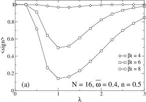
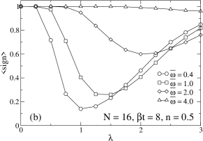
Figure 12: Average sign $\langle\text{sign}\rangle$ [Eq. (27)] of the fermionic weight $w_{\text{f}}$ as a function of electron-phonon coupling $\lambda$ in one dimension (a) for different inverse temperatures $\beta$, and (b) for different values of the adiabatic ratio $\overline{\omega}_{0}$. Here and in subsequent figures $\Delta\tau=0.05$, lines are guides to the eye only, and errorbars are suppressed if smaller than the symbols shown.

A.3 Sign problem

Since a possible sign problem crucially affects QMC simulations, this section is devoted to a detailed investigation of the dependence of the average sign on the various parameters.

While Hamiltonian (5) is symmetric with respect to a particle-hole transformation for $\mu=-E_{\text{P}}$ (half filling), this symmetry is broken if we use the checkerboard approximation (10), so that $n\neq 0.5$ for the above choice of the chemical potential. To simplify calculations, the results for the average sign at $n=0.5$ presented below have therefore been obtained using the exact hopping term. For general band fillings, we find that the checkerboard breakup requires different values of $\mu$ to perform simulations at the same electron densities, but results are identical within statistical errors if $\mu$ is adjusted accordingly.

The derivation of the QMC algorithm in Sec. A.1 is valid for any dimension D of the lattice under consideration. Nevertheless, here we only report results for the sign problem in $\text{D}=1$, the case considered in Sec. IV, and make some remarks about the influence of the dimensionality at the end.

The average sign is defined as

$$\langle\text{sign}\rangle=\frac{\langle w_{\text{f}}\rangle_{\text{b}}}{\langle|w_{\text{f}}|\rangle_{\text{b}}}\,,$$ (27)

with the fermionic weight in the present case given by $w_{\text{f}}=\det(1+\Omega)$ [Eq. (8)]. We begin with the dependence of $\langle\text{sign}\rangle$ on the electron-phonon coupling strength. For simplicity, we show results for $n=0.5$, while the effect of band filling will be discussed later. The choice $n=0.5$ is convenient since we know the chemical potential, and we shall see below that the sign problem is most pronounced for a half-filled band. Moreover, all existing QMC results for the spinless Holstein model are for half filling, so that it is interesting to see how the sign problem affects simulations within the current approach.

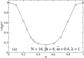
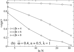
Figure 13: Average sign as a function of (a) band filling $n$, and (b) system size $N$.

Figure 12(a) reveals that the average sign takes on a minimum near the point where—depending on the filling—the cross over to small polarons or a CDW state occurs. In the adiabatic regime $\overline{\omega}_{0}<1$, the cross over condition is $\lambda>1$ [Fig. 12(a)], whereas for $\overline{\omega}_{0}>1$ we have $g>1$ [Fig. 12(b)]. At weak and strong coupling, the average sign is close to 1, so that accurate simulations can be carried out. As shown in Fig. 12(b), we find that $\langle\text{sign}\rangle$ becomes very small for $\overline{\omega}_{0}<1$ and intermediate $\lambda$, while it increases noticeably in the nonadiabatic regime $\overline{\omega}_{0}>1$. Owing to the absence of any autocorrelations in our approach, the present method therefore represents a significant improvement of existing algorithms, as the latter face severe autocorrelations even for $\overline{\omega}_{0}\gtrsim 1$, thereby limiting the temperature range and cluster size.

As illustrated in Fig. 13(a), the average sign depends strongly on the band filling $n$. While $\langle\text{sign}\rangle\approx 1$ in the vicinity of $n=0$ or $n=1$, a significant reduction is visible near half filling $n=0.5$. The minimum occurs at $n=0.5$, and the results display particle-hole symmetry as expected. Here we have chosen $\beta t=8$, $\overline{\omega}_{0}=0.4$ and $\lambda=1$, for which the sign problem is most noticeable according to Fig. 12. Note that there is no sign problem in simulations for, e.g., the Hubbard model at half filling, where the (fermionic) weights of the $\uparrow$ and $\downarrow$ electrons are equal and their product—entering the partition function—is positive.von der Linden (1992) This can also be expected within the current approach if we consider the half–filled spinfull Holstein or Holstein-Hubbard model, and work along this line is in progress.

Finally, in Fig. 13(b), we report the average sign as a function of system size, again for $n=0.5$. The behavior is strikingly different from the one-electron case considered in I. While in the latter $\langle\text{sign}\rangle\rightarrow 1$ as $N\rightarrow\infty$, here the average sign decreases nearly exponentially with increasing system size. Obviously, this limits the applicability of our method. However, as illustrated in Sec. IV, we can nevertheless obtain accurate results at low temperatures, small phonon frequencies, and over a large range of the electron-phonon interaction. Moreover, we would like to point out that for such parameters, existing methods suffer strongly from autocorrelations, rendering simulations extremely difficult.

The dependence of the sign problem on the dimension of the system is similar to the single-electron case.Hohenadler et al. (2004) For the same parameters $N$, $\overline{\omega}_{0}$, $\beta t$ and $\lambda$, the minimum in $\langle\text{sign}\rangle$ at intermediate $\lambda$ becomes more pronounced as one increases the dimension of the cluster.

To conclude with, we would like to point out that, in principle, the sign problem can be compensated by performing sufficiently long QMC runs, although we have to keep in mind that the statistical errors increase proportional to $\langle\text{sign}\rangle^{-2}$ (Ref. von der Linden, 1992). Owing to the purely phononic updates, the present algorithm is very fast and we have made up to about $2.6\times 10^{7}$ single measurements to obtain the results presented in Sec. IV. The use of the reweighting method requires us to store the measured values of observables in every MC step, and to perform the Jackknife error analysisDavison and Hinkley (1997) at the end of the run. For example, in the case of the Green function (20), $L+1$ complex numbers have to be stored for each momentum $k$ in every step. Depending on the observables of interest, this sets a practical limit for the maximal number of measurements due to restrictions in available disk space.

References

- Bar-Yam et al. (1992) Y. Bar-Yam, J. Mustre de Leon, and A. R. Bishop, eds., Lattice Effects in High Temperature Superconductors (World Scientific, Singapore, 1992).
- Edwards (2002) D. M. Edwards, Adv. Phys. 51, 1259 (2002).
- Hartinger et al. (2004) C. Hartinger, F. Mayr, J. Deisenhofer, A. Loidl, and T. Kopp, Phys. Rev. B 69, R100403 (2004).
- Hartinger et al. (unpublished) C. Hartinger, F. Mayr, A. Loidl, and T. Kopp, cond-mat/0406123 (unpublished).
- Tempere and Devreese (2001) J. Tempere and J. T. Devreese, Phys. Rev. B 64, 104504 (2001).
- De Raedt and Lagendijk (1982) H. De Raedt and A. Lagendijk, Phys. Rev. Lett. 49, 1522 (1982).
- De Raedt and Lagendijk (1983) H. De Raedt and A. Lagendijk, Phys. Rev. B 27, 6097 (1983).
- Kabanov and Mashtakov (1993) V. V. Kabanov and O. Y. Mashtakov, Phys. Rev. B 47, 6060 (1993).
- Fehske et al. (1995) H. Fehske, H. Röder, G. Wellein, and A. Mistriotis, Phys. Rev. B 51, 16 582 (1995).
- Romero et al. (1999) A. H. Romero, D. W. Brown, and K. Lindenberg, Phys. Rev. B 60, 14080 (1999).
- Cataudella et al. (1999) V. Cataudella, G. De Filippis, and G. Iadonisi, Phys. Rev. B 60, 15 163 (1999).
- Cataudella et al. (2001) V. Cataudella, G. De Filippis, and G. Iadonisi, Phys. Rev. B 63, 52406 (2001).
- Fröhlich (1954) H. Fröhlich, Adv. Phys. 3, 325 (1954).
- Alexandrov and Kornilovitch (1999) A. S. Alexandrov and P. E. Kornilovitch, Phys. Rev. Lett. 82, 807 (1999).
- Bonča et al. (2000) J. Bonča, T. Katrašnik, and S. A. Trugman, Phys. Rev. Lett. 84, 3153 (2000).
- Hirsch and Fradkin (1982) J. E. Hirsch and E. Fradkin, Phys. Rev. Lett. 49, 402 (1982).
- Hirsch and Fradkin (1983) J. E. Hirsch and E. Fradkin, Phys. Rev. B 27, 4302 (1983).
- McKenzie et al. (1996) R. H. McKenzie, C. J. Hamer, and D. W. Murray, Phys. Rev. B 53, 9676 (1996).
- Weiße and Fehske (1998) A. Weiße and H. Fehske, Phys. Rev. B 58, 13 526 (1998).
- Bursill et al. (1998) R. J. Bursill, R. H. McKenzie, and C. J. Hamer, Phys. Rev. Lett. 80, 5607 (1998); H. Fehske, M. Holicki, and A. Weiße, Adv. Solid State Phys. 40, 235 (2000).
- Zheng et al. (1989) H. Zheng, D. Feinberg, and M. Avignon, Phys. Rev. B 39, 9405 (1989).
- Feinberg et al. (1990) D. Feinberg, S. Ciuchi, and F. de Pasquale, Int. J. Mod. Phys. B 4, 1317 (1990).
- Zheng and Avignon (1998) H. Zheng and M. Avignon, Phys. Rev. B 58, 3704 (1998).
- Wang et al. (2000) Q. Wang, H. Zheng, and M. Avignon, Phys. Rev. B 63, 014305 (2000).
- Perroni et al. (2003) C. A. Perroni, V. Cataudella, G. De Filippis, G. Iadonisi, V. Marigliano Ramaglia, and F. Ventriglia, Phys. Rev. B 67, 214301 (2003).
- Capone et al. (1999) M. Capone, M. Grilli, and W. Stephan, Eur. Phys. J. B 11, 551 (1999).
- Fehske et al. (1994) H. Fehske, D. Ihle, J. Loos, U. Trapper, and H. Büttner, Z. Phys. B 94, 91 (1994); H. Fehske, Habilitation Thesis, University Bayreuth (1996).
- Hohenadler et al. (2004) M. Hohenadler, H. G. Evertz, and W. von der Linden, Phys. Rev. B 69, 024301 (2004).
- Lang and Firsov (1962) I. G. Lang and Y. A. Firsov, Zh. Eksp. Teor. Fiz. 43, 1843 (1962), [Sov. Phys. JETP 16, 1301 (1962)].
- Kornilovitch (1997) P. E. Kornilovitch, J. Phys.: Condens. Matter 9, 10675 (1997).
- Jarrell and Gubernatis (1996) M. Jarrell and J. E. Gubernatis, Phys. Rep. 269, 133 (1996).
- von der Linden et al. (1999) W. von der Linden, R. Preuss, and V. Dose, in Maximum Entropy and Bayesian Methods, edited by W. von der Linden, V. Dose, R. Fischer, and R. Preuss (Kluwer Academic Publishers, Dordrecht, 1999).
- Silver et al. (1990) R. N. Silver, D. S. Sivia, and J. E. Gubernatis, Phys. Rev. B 41, 2380 (1990).
- von der Linden et al. (1996) W. von der Linden, R. Preuss, and W. Hanke, J. Phys.: Condens. Matter 8, 3881 (1996).
- Bäuml et al. (1998) B. Bäuml, G. Wellein, and H. Fehske, Phys. Rev. B 58, 3663 (1998).
- Robin (1997) J. M. Robin, Phys. Rev. B 56, 13 634 (1997).
- Sykora et al. (2005) S. Sykora, A. Hübsch, K. W. Becker, G. Wellein, and H. Fehske, Phys. Rev. B 71, 045112 (2005).
- Stephan (1996) W. Stephan, Phys. Rev. B 54, 8981 (1996).
- Wellein and Fehske (1997) G. Wellein and H. Fehske, Phys. Rev. B 56, 4513 (1997).
- Hohenadler et al. (2003) M. Hohenadler, M. Aichhorn, and W. von der Linden, Phys. Rev. B 68, 184304 (2003).
- Alexandrov and Ranninger (1992) A. S. Alexandrov and J. Ranninger, Phys. Rev. B 45, 13 109 (1992).
- Kornilovitch (2002) P. E. Kornilovitch, Europhys. Lett. 59, 735 (2002).
- White (1991) S. R. White, Phys. Rev. B 44, 4670 (1991).
- Capone et al. (1997) M. Capone, W. Stephan, and M. Grilli, Phys. Rev. B 56, 4484 (1997).
- Ciuchi et al. (1997) S. Ciuchi, F. de Pasquale, S. Fratini, and D. Feinberg, Phys. Rev. B 56, 4494 (1997).
- De Raedt and Lagendijk (1986) H. De Raedt and A. Lagendijk, Z. Phys. B: Condens. Matter 65, 43 (1986).
- von der Linden (1992) W. von der Linden, Phys. Rep. 220, 53 (1992).
- Blankenbecler et al. (1981) R. Blankenbecler, D. J. Scalapino, and R. L. Sugar, Phys. Rev. D 24, 2278 (1981).
- dos Santos (2003) R. R. dos Santos, Braz. J. Phys. 33, 36 (2003).
- Loh and Gubernatis (1992) E. Y. Loh and J. E. Gubernatis (Elsevier Science Publishers, North-Holland, Amsterdam, 1992).
- Hirsch (1985) J. E. Hirsch, Phys. Rev. B 31, 4403 (1985).
- Davison and Hinkley (1997) A. C. Davison and D. V. Hinkley, Bootstrap Methods and their Application (Cambridge University Press, Cambridge, UK, 1997).