Optical orientation of electron spins in GaAs quantum wells

Abstract

We present a detailed experimental and theoretical analysis of the optical orientation of electron spins in GaAs/AlAs quantum wells. Using time and polarization resolved photoluminescence excitation spectroscopy, the initial degree of electron spin polarization is measured as a function of excitation energy for a sequence of quantum wells with well widths between $63$ Å and $198$ Å. The experimental results are compared with an accurate theory of excitonic absorption taking fully into account electron-hole Coulomb correlations and heavy-hole light-hole coupling. We find in wide quantum wells that the measured initial degree of polarization of the luminescence follows closely the spin polarization of the optically excited electrons calculated as a function of energy. This implies that the orientation of the electron spins is essentially preserved when the electrons relax from the optically excited high-energy states to quasi-thermal equilibrium of their momenta. Due to initial spin relaxation, the measured polarization in narrow quantum wells is reduced by a constant factor that does not depend on the excitation energy.

I Introduction

The optical excitation of semiconductors with circularly polarized light creates spin-polarized electrons in the conduction band. Dyakonov and Perel (1984) The degree of electron spin polarization obtainable by means of optical orientation can reach almost $100$%, depending on the conduction and valence band states involved in the optical transition. The intimate relation between electron spin and circularly polarized light has formed the basis for many of the pioneering experiments of semiconductor spintronics. Optical investigations demonstrated the efficient injection of spin polarized electrons,Oestreich et al. (1999); Fiederling et al. (1999) the transport of spin polarized electrons over macroscopical distances,Hägele et al. (1998); Kikkawa and Awschalom (1999) manipulation and storage of spin orientation,Salis et al. (2001) and the interaction with nuclear momenta Lampel (1968). Furthermore, the spin dependence of optical transitions can be utilized to switch the intensity and polarization of a semiconductor laser by changing the spin orientation of injected electrons.Hallstein et al. (1997) Recently, the reduction of the threshold in semiconductor lasers pumped with spin-polarized electrons was observed.Rudolph et al. (2003) But although optical orientation has proven to be a powerful tool to study electron spins in quasi-two-dimensional (quasi-2D) semiconductor systems, the present understanding of spin orientation is based on crude approximations. A direct comparison of experimentally determined degrees of spin orientation with an accurate theoretical treatment is still missing. The goal of this paper is thus to present a systematic experimental and theoretical study of the optical orientation of electron spins in quasi-2D systems.

In direct semiconductors like GaAs, the selection rules for optical transitions from the uppermost valence band to the lowest conduction band are commonly based on the simple picture that the electron states in the conduction band have spin $S=1/2$ whereas the hole states in the valence band have an effective spin $S=3/2$. The hole states with spin $z$-component $S_{z}=\pm 3/2$ are denoted heavy-hole (HH) states whereas the light-hole (LH) states have $S_{z}=\pm 1/2$. For absorption and emission of circularly polarized light we thus get the selection rules depicted in Fig. 1 (Ref. Dyakonov and Perel, 1984). According to this scheme, the transition probability from the HH states to the conduction band is three times larger than from the LH states. In bulk semiconductors, we thus expect that the maximum attainable degree of spin polarization is $P_{s}=0.5$, where $P_{s}$ is defined as

$$P_{s}=\frac{N_{+}-N_{-}}{N_{+}+N_{+}}\,,$$ (1)

and $N_{+}$ ($N_{-}$) is the number of electrons with spin up (down), respectively. In 2D systems the degeneracy of the HH and LH states is lifted as sketched in Fig. 1. For resonant excitation at the HH energy we thus expect a rise of the maximum attainable degree of polarization up to $P_{s}=1$.

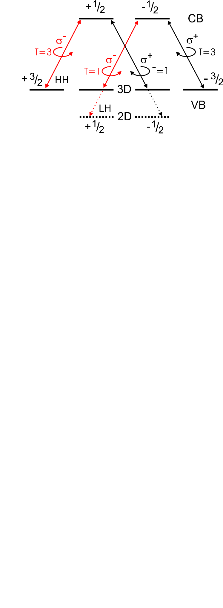
Figure 1: Selection rules and relative transition rates $T$ for optical transitions between valence band (VB) states having an effective spin $S=3/2$ and conduction band (CB) states with $S=1/2$ (Ref. Dyakonov and Perel, 1984). In bulk semiconductors the HH states ($S_{z}=\pm 3/2$) are degenerate with the LH states ($S_{z}=\pm 1/2$) whereas in quasi-2D systems the LH states (dotted bold lines) are lower in energy than the HH states.

Even in a single-particle picture for the optical excitation, the naive $3:1$ ratio of HH and LH transitions is obtained only if HH-LH coupling of the hole states at nonzero wave vectors $\bm{k}$ is neglected. Due to this HH-LH coupling, the hole states with $k>0$ are not spin eigenstates. Furthermore, a realistic treatment must take into account that optical absorption gives rise to the formation of excitons, i.e., Coulomb correlated electron-holes pairs. Thus even for excitations close to the absorption edge we get substantial HH-LH coupling because the exciton states consist of electron and hole states with $k$ of the order of $1/a_{\mathrm{B}}^{\ast}$, where $a_{\mathrm{B}}^{\ast}$ is the effective Bohr radius. The Coulomb coupling between electron and hole states yields a second contribution to the mixing of single particle states with different values of $S_{z}$. Finally, we must keep in mind that for higher excitation energies we get a superposition of exciton continua that are predominantly HH- or LH-like. These different excitons contribute oppositely to the spin orientation of electrons. We note that these arguments are valid for the optical excitation of bulk semiconductors and quasi-2D systems.

In early works, several groups Weisbuch et al. (1981); Masselink et al. (1984) reported on polarization resolved transmission and photoluminescence (PL) experiments on GaAs/AlGaAs quantum wells (QWs) under cw excitation. They measured the polarization as a function of excitation energy for a small range of excess energies. In later works, the electron spin polarization $P_{s}$ in quasi-2D systems was studied using time-resolved photoluminescence excitation spectroscopy. For excitation energies even slightly above the HH resonance, several authors Freeman et al. (1990); Dareys et al. (1993); Muñoz et al. (1995) observed a polarization $P_{s}$ that was significantly smaller than one. These measurements were carried out on fairly narrow GaAs/AlGaAs multiple QWs with well widths $w=40$ Å (Refs. Freeman et al., 1990; Dareys et al., 1993) and $77$ Å (Ref. Muñoz et al., 1995). A first well-width dependent study of optical orientation was performed experimentally by Roussignol et al., Roussignol et al. (1992) but only for excitation energies up to $30$ meV above the HH resonance. For energies near the HH resonance, Roussignol et al. found initial spin polarizations in the range $60-80$%, whereas they expected values between $85$ and $90$%. They argued that additional relaxation mechanisms were required to describe their results. Kohl et al. Kohl et al. (1991) studied the optical orientation in an $80$ Å wide GaAs QW for an excess energy of $\Delta E=60$ meV above the HH absorption edge. In contrast to our findings discussed below, they observed for this value of $\Delta E$ a rather large initial spin polarization close to $100$%.

Twardowski and Hermann Twardowski and Hermann (1987) as well as Uenoyama and Sham Uenoyama and Sham (1990) studied the polarization of QW PL theoretically, taking into account HH-LH coupling in the valence band. However, these authors neglected the Coulomb interaction between electron and hole states. On the other hand, Maialle et al. Maialle et al. (1993) investigated the spin dynamics of excitons taking into account the exchange coupling between electrons and holes, but they disregarded the HH-LH coupling in the valence band. Both the HH-LH coupling and the Coulomb coupling are known to be important for an accurate description of excitonic spectra. Winkler (1995) To the best of our knowledge, no systematic experimental or theoretical examination of $P_{s}$ for different well widths and a wide range of excitation energies has been reported so far.

In this work we experimentally analyze the energy dependence of the optical selection rules for the creation and recombination of spin polarized carriers by investigating the time-dependent polarized luminescence of seven $(100)$ GaAs/AlAs QWs with well widths from $63$ to $198$ Å and excitation energies between $1.529$ and $1.744$ eV. We compare these results with an accurate theory of excitonic absorption taking into account Coulomb coupling and HH-LH coupling between the subbands. Winkler (1995) The experimental results for a wide range of parameters are in good agreement with the parameter-free calculations. We find that the measured initial optical polarization of the luminescence follows closely the spin polarization of the optically excited electrons calculated as a function of energy. This implies that the orientation of the electron spins is essentially preserved when the electrons relax from the optically excited high-energy states to quasi-thermal equilibrium of their momenta. In narrow QWs, however, the measured polarization is reduced due to fast initial spin relaxation that is almost independent of the excitation energy.

The paper is organized as follows. Section II describes the experimental setup and the sample under investigation. In Sec. III, we first present the results for a $198$ Å wide QW where we obtain very good agreement between experiment and theory. Second, we discuss how the polarization observed in narrow QWs is reduced because of fast initial spin relaxation directly after laser excitation. Our theory for optical orientation is introduced in Sec. IV, where we give a detailed discussion of the influence of Coulomb coupling and HH-LH coupling for an accurate theoretical description of the optical orientation of electron spins. The conclusions are summarized in Sec. V.

II Experimental Methods

The sample under investigation is a high quality intrinsic GaAs/AlAs structure containing twelve single QWs with different well widths grown by MBE on a $(100)$ oriented GaAs substrate. Sogawa et al. (2001) The QWs are separated by a triple layer of $26$ Å AlAs, $27$ Å GaAs, and $26$ Å AlAs. In this work we present experimental data for the seven broadest QWs with well widths between $63$ and $198$ Å.wel The sample is mounted in a finger cryostat and all measurements were performed at a temperature of $4.2$ K. Pulses from a Kerr-lens mode-locked Ti:sapphire laser excite the sample with a repetition rate of $80$ MHz. We use a pulse shaper to reduce the spectral linewidth of the $100$ fs pulses to $0.8$ nm full width at half maximum (FWHM). The wavelength is tuned from $711$ nm to $811$ nm in steps of 1 nm. The maximum excitation power is limited to about $2$ mW, because most of the laser power is blocked by the pulse shaper. We estimate that the optically excited carrier density lies in the range $2\times 10^{8}-2\times 10^{9}$ cm^-2 depending on the QW width and the excitation energy. We carefully control the polarization of the exciting laser pulse by means of a Soleil-Babinet polarization retarder, taking into account the dependence of the retardation on the excitation wavelength. The retarder is readjusted for each excitation wavelength to achieve close to 100% circularly polarized light. The PL is measured in reflection geometry by a synchroscan streak camera providing a spectral and temporal resolution of $7$ meV and $15$ ps, respectively. We separately detect the two circularly polarized PL components $\sigma^{\pm}$ using an electrically tunable liquid-crystal retarder. Each QW emits light only at its energetically lowest excitonic resonance. Since the PL wavelengths of the QWs vary over a wide range and the liquid-crystal retarder shows a chromatic dependence of the retardation, the PL data were corrected independently for each QW according to the measured dispersion curve of the retarder.

We obtain the time dependent degree of optical polarization

$$P_{\mathrm{opt}}(t)=\frac{I_{+}(t)-I_{-}(t)}{I_{+}(t)+I_{-}(t)}$$ (2)

from the time resolved PL spectra, where $I_{\pm}(t)$ is the PL intensity of the $\sigma^{\pm}$ component. $P_{\mathrm{opt}}(t)$ is measured for each QW scanning the excitation energy from $1.529$ to $1.744$ eV. As an example, Fig. 2 shows $P_{\mathrm{opt}}(t)$ for the $152$ Å QW at an excitation energy of $1.744$ eV which corresponds to an excess energy of $209$ meV above the lowest HH resonance. We determine the initial degree of polarization by fitting $P_{\mathrm{opt}}(t)$ to

$$P_{\mathrm{opt}}(t)=P_{1}+P_{0}\exp(-t/\tau_{s})\,,$$ (3)

where $\tau_{s}$ is the decay time of $P_{\mathrm{opt}}(t)$. We identify $P_{0}$ with the optical polarization at $t=0$. $P_{1}$ corresponds to an offset in the measurement of usually below $0.02$ which is probably due to a slight linear polarization introduced by the liquid crystal retarder. The error $P_{1}$ is included in the error bars of $P_{0}$.

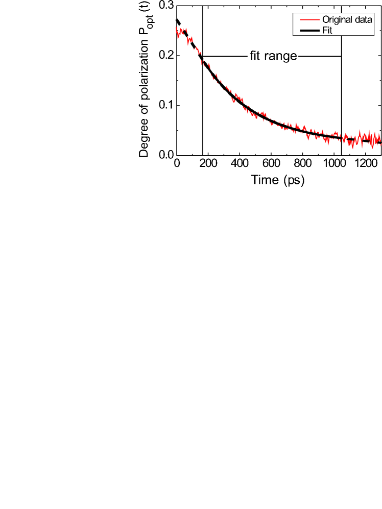
Figure 2: Time dependent degree of polarization $P_{\mathrm{opt}}(t)$ for the $152$ Å wide QW at an excitation energy of $1.744$ eV (red line) and exponential fit based on Eq. (3) (black line).

The central idea underlying the interpretation of our experiments is that we can identify the measured degree of optical polarization with the electron spin polarization, $P_{\mathrm{opt}}(t)=P_{s}(t)$. This association is based on the following arguments. First we recall that the electron spin relaxation is usually slow compared to the hole spin relaxation. Damen et al. (1991) Therefore, every electron can radiatively recombine with an appropriate hole state. Second we note that the measured PL reflects only the HH1:E1(1s) transition. [In this paper we label optical transitions by the hole (HH or LH) and electron (E) subbands contributing dominantly to the excitonic states. For a bound exciton we append in brackets the quantum number of the bound state. Winkler (1995) See also the discussion in Sec. IV.] Our calculations indicate that for this transition we have a strict one-to-one correspondence between the spin polarization and the degree of optical orientation, with completely spin polarized electrons giving rise to perfectly circularly polarized light. This is confirmed by the experiments showing a very high degree of optical polarization for the HH1:E1 transition. Third, we assume that the electron spin polarization is preserved during the first few ps after laser excitation while the electrons relax from the optically excited high-energy states to quasi-thermal equilibrium for the momenta. This assumption is best fulfilled in wide QWs, see our discussion of initial spin relaxation in Sec. III.2. Finally, we remark that the above arguments imply that the decay time $\tau_{s}$ in Eq. (3) can be identified with the spin relaxation time of the electrons.

III Results and discussion

III.1 Initial degree of polarization

In this section we will discuss optical spin orientation for the $198$ Å QW. Here, the excitation power is $200$ $\mu$W and the laser spot radius is approximately $125~{}\mu$m which creates a low carrier density of the order of $5\times 10^{8}$ cm^-2. We choose this low excitation power to avoid a spectral overlap of the PL from the substrate with the PL from the QW. Figure 3 shows the measured [Fig. 3(a)] and the calculated [Fig. 3(b)] degree of spin polarization as a function of excitation energy. For comparison, the solid line in Fig. 3(c) shows the calculated absorption spectrum $\alpha(\omega)$ for $\sigma^{-}$ polarized light. While the solid line contains contributions from all dipole allowed exciton states at energy $\hbar\omega$, the broken lines differentiate between the contributions of those states to $\alpha(\omega)$, whose electron spin is oriented either up or down. In agreement with Fig. 1, these contributions are essentially the same as the contributions of HH and LH states to $\alpha(\omega)$. The partitioning of $\alpha(\omega)$ combined with the calculated electron and hole subband energies allows us to label the peaks in the polarization spectra in Figs. 3(a) and 3(b) by the electron (E) and hole (HH or LH) subbands. The solid vertical lines in Fig. 3 indicate the identified peaks. A more detailed discussion of the labeling scheme will be given in Sec. IV.

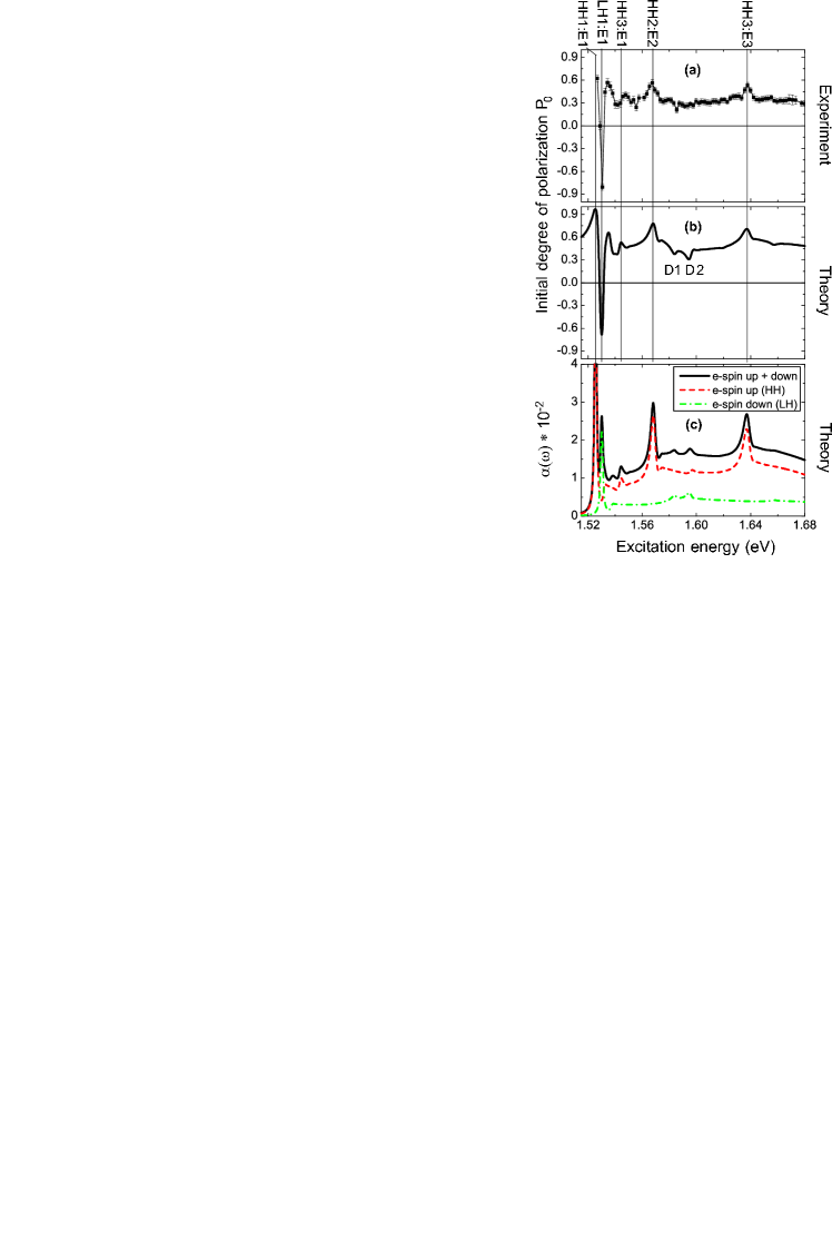
Figure 3: (a) Measured and (b) calculated initial degree of spin polarization $P_{0}$ as a function of excitation energy of the $198$ Å wide GaAs/AlAs QW. The vertical lines label the resonances in (a) and (b) according to the dominantly contributing electron (E) and hole (LH or HH) subbands as discussed in Sec. IV. The black line in (c) shows the calculated absorption coefficient $\alpha(\omega)$. The red dashed line (green dash-dotted line) in (c) shows how excitons containing spin up (spin down) electrons contribute to $\alpha(\omega)$.

The first positive peak at 1.525 eV corresponds to the HH1:E1(1s) transition. Next we find a narrow region around 1.53 eV with negative $P_{0}$ which we attribute to the LH1:E1(1s) transition. For the 198 Å wide QW investigated here the LH1:E1(1s) exciton is below the continuum of HH1:E1 excitons so that the LH1:E1(1s) exciton is a discrete state (i.e., not a Fano resonance). Therefore, $|P_{0}|$ is smaller than one only due to the homogenous broadening of the exciton states. The next peak at 1.535 eV reflects the absorption edge of the HH1:E1 exciton continuum. The LH component in Fig. 3(c) exhibits a minimum which explains the large positive value of $P_{0}$. The LH1:E1 absorption edge at 1.539 eV, along with the decreasing HH contribution, leads to a reduction of $P_{0}$ followed by a peak at 1.544 eV which corresponds to the HH3:E1(1s) transition. We attribute the following peak at 1.568 eV to the HH2:E2(1s) transition, while the peak at 1.637 eV corresponds to the HH3:E3(1s) transition. All these structures are found in both experiment and theory.

Interestingly, theory shows a dip of $P_{0}$ at 1.584 eV labeled D1 in Fig 3(b) which appears to be related to a transition from an LH state to the conduction band. However, unlike the transitions discussed above, it cannot be related to a particular pair of electron and hole subbands. Furthermore, we observe a dip of $P_{0}$ at 1.595 eV (D2) in Fig. 3(b). The calculations indicate that two excitons are almost degenerate at this energy, the LH2:E2(1s) and the HH4:E2 exciton with the latter being slightly higher in energy. (We remark that, strictly speaking, all excitons above the HH1:E1 absorption edge at $1.535$ eV are Fano resonances. Winkler (1995))

Finally we note that there is a very good agreement between experiment and theory not only for the individual features in the spectra, but also for the relative height of the peaks and the general trends of $P_{0}$ as a function of energy. The good agreement between the experimental data and the calculated results shows that our theory provides a realistic picture of the spin and energy dependent optical selection rules in GaAs QWs. In Sec. IV we show that it is vital for our quantitative theory to take into account both Coulomb coupling and HH-LH coupling. If these couplings are neglected, we get substantial deviations between experiment and theory.

III.2 Initial spin relaxation

In Sec. II we identified the measured degree of optical polarization with the spin orientation of excited electrons based on the assumption that the electron spin polarization is preserved when the electrons relax from high-energy states to thermal equilibrium. This assumption is well fulfilled for wide QWs (see Fig. 3) where we obtained good agreement between absolute values of the measured and calculated spin polarization $P_{0}$. Figure 4 shows the measured and calculated $P_{0}$ for the QWs with well widths between $152$ and $63$ Å and an excitation power of $1$ mW. Once again, we obtain good agreement between experiment and theory for many features in the spectra. The ratio between measured and calculated values decreases, however, with decreasing well width. The ratio is close to one for the $198$ Å wide QW, but becomes much smaller for the narrow QWs. Interestingly, this ratio is for each QW approximately constant for a large range of energies. We propose that the reduced value of $P_{0}$ is due to fast initial spin relaxation of the excited electrons prior to establishing thermal equilibrium for their momenta.

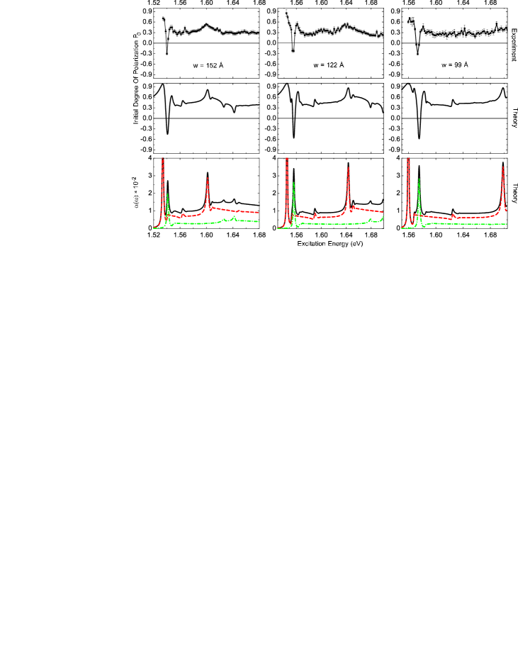
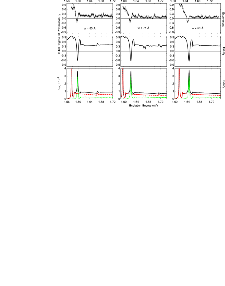
Figure 4: Initial degree of spin polarization $P_{0}$ as a function of excitation energy for GaAs/AlAs QWs with different well widths. The upper panels show experimental data measured at an excitation power of 1 mW, the central panels are calculated results. For comparison, the black lines in the lower panels show the calculated absorption coefficient $\alpha(\omega)$. The red dashed line (green dash-dotted line) in the lower panels show how excitons containing spin up (spin down) electrons contribute to $\alpha(\omega)$, see Eq. (14).

We assume that this mechanism is similar to the Dyakonov-Perel (DP) spin relaxation of electrons. Dyakonov and Perel (1972) An excitation with energies above the HH1:E1 resonance creates electrons with large wave vectors $\bm{k}_{\|}$. In these states, the electron spins are exposed to an effective magnetic field $\bm{\Omega}(\bm{k}_{\|})$ due to the conduction band spin splitting. While the electrons relax from the excited states to states in thermal equilibrium with smaller wave vectors $\bm{k}_{\|}$, the spins precess around the field $\bm{\Omega}(\bm{k}_{\|})$ so that the measured spin orientation is reduced. We call this process initial spin relaxation. Muñoz et al. (1995) We note that, in general, DP spin relaxation becomes more efficient for larger electron energies so that the time scale of the initial spin relaxation is shorter than the spin relaxation time $\tau_{s}$ at later times (compare Figure 2).

To obtain a qualitative estimate of how the initial spin relaxation influences the measured polarization $P_{0}$, we evaluate the average spin precession period $T_{z}$ of the optically excited electron states prior to the first scattering event. In the following, we consider only inelastic scattering processes with energy relaxation time $\tau_{E}$ and neglect the motional narrowing so that the calculated precession period $T_{z}$ is a lower bound for the time scale of the inital spin relaxation (cf. Sec. III.3). Furthermore, we neglect Coulomb coupling so that the electron states can be characterized by the in-plane wave vector $\bm{k}_{\|}$.

We start with the expression for the effective magnetic field vector in symmetric (100)-oriented QWs Kainz et al. (2003)

$$\bm{\Omega}(\bm{k}_{\|})=\frac{2\gamma}{\hbar}\left(\begin{array}[]{c}k_{x}\left(k_{y}^{2}-\langle k_{z}^{2}\rangle\right)\\[2.15277pt] k_{y}\left(\langle k_{z}^{2}\rangle-k_{x}^{2}\right)\\[2.15277pt] 0\end{array}\right),$$ (4)

where $\bm{k}_{\|}=(k_{x},k_{y},0)$ is the in-plane wave vector, $k_{z}$ is the quantized perpendicular component of $\bm{k}$, and $\gamma$ is the Dresselhaus coefficient. For an isotropic dispersion we obtain the average precession frequency $\langle\Omega_{z}\rangle(k_{\|})$ of electron spins polarized in $z$ direction by averaging $|\bm{\Omega}(\bm{k}_{\|})|$ over the polar angle $\phi$ of $\bm{k}_{\|}=k_{\|}(\cos\phi,\sin\phi,0)$

$$\langle\Omega_{z}\rangle(k_{\|})=\frac{1}{2\pi}\int_{0}^{2\pi}\mathrm{d}\phi\,\left|\Omega\left(\bm{k}_{\|}\right)\right|.$$ (5)

Assuming a parabolic dispersion of the electron excess energy, $\Delta E=\hbar^{2}k_{\|}^{2}/(2m^{\ast})$ with effective mass $m^{\ast}$, we can express the precession period $T_{z}=2\pi/\langle\Omega_{z}\rangle$ in terms of $\Delta E$.

The quantity $T_{z}$ provides an estimate for the timescale on which the optically induced spin orientation is lost. It competes with the timescale $\tau_{E}$ of the energy relaxation. We can estimate the ratio between the measured and the optically excited spin polarization by calculating

$$R(k_{\|}) = \begin{array}[t]{>{\displaystyle}r}\frac{1}{\tau_{E}(k_{\|})}\int\frac{\mathrm{d}\phi}{2\pi}\int_{0}^{\infty}\mathrm{d}t\,\exp\left[-t/\tau_{E}(k_{\|})\right]\\ \times\cos\left[|\Omega(\bm{k}_{\|})|\,t\right]\end{array}$$ (6c)

$$= \int\frac{\mathrm{d}\phi}{2\pi}\;\frac{1}{1+|\Omega(\bm{k}_{\|})|^{2}\,\tau_{E}^{2}(k_{\|})}\,,$$ (6d)

where we have assumed that the occupation of the initially excited states $\bm{k}_{\|}$ decreases exponentially with decay time $\tau_{E}$. For $\tau_{E}\ll T_{z}$ we obtain $R(k_{\|})\approx 1-(2\pi\tau_{E}/T_{z})^{2}$.

The spin precession period $T_{z}$ as a function of excess energy $\Delta E$ is shown in Fig. 5. For a more quantitative treatment of initial spin relaxation, we would need to know the energy relaxation time $\tau_{E}$. We cannot determine $\tau_{E}$ experimentally as it is shorter than the temporal resolution of our experimental setup. Furthermore, an estimate is hindered by the fact that $\tau_{E}$ depends not only on the wave vector $k_{\|}$ but also on other parameters such as the number of scattering centers, the carrier mobility and density. Therefore, a quantitative comparison of Eq. (6) with our experimental results is hardly possible. Nonetheless, we can draw the following qualitative conclusions from the above model.

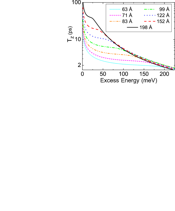
Figure 5: Average spin precession time $T_{z}=2\pi/\langle\Omega_{z}\rangle$ as a function of excess energy $\Delta E$ for different QWs with well widths between $63$ and $198$ Å.

First we discuss the regime of excess energies $\Delta E\leq 50$ meV. For wide QWs with well widths between $198$ and $122$ Å we obtain relatively large values of $T_{z}\gtrsim 10$ ps. Assuming a typical energy relaxation time $\tau_{E}\approx 200$ fs, Eq. (6) yields a maximum decrease of $P_{0}$ of $\lesssim 3$% so that the influence of initial spin relaxation can be neglected for these wide wells. Narrow QWs with well widths $\leq 71$ Å exhibit short precession times $T_{z}\lesssim 4$ ps. This is due to the increase of $\langle k_{z}^{2}\rangle$ with decreasing QW width, which causes a larger effective field $|\Omega(\bm{k}_{\|})|$ according to Eq. (4). Consistent with these results, Eq. (6) predicts a large decrease of $P_{0}$ of about $50$ % in narrow wells, in good qualitative agreement with the experimental findings.

For excess energies $\Delta E>50$ meV we obtain $T_{z}\approx\mathrm{const}$ for QW widths $\leq 83$ Å. Here the $k_{\|}$-linear terms in Eq. (5) are compensated by the $k_{\|}^{3}$ terms. This explains why the ratio between theoretical and experimental values of $P_{0}$ is approximately constant as a function of $\Delta E$. For the wide QWs, $T_{z}$ shows a decrease for $\Delta E>50$ meV. This is easily explained by the increasing contribution of the $k_{\|}^{3}$ terms in Eq. (5). If $k_{\|}^{2}\gg\langle k_{z}^{2}\rangle$ we expect therefore a strong influence of initial spin relaxation even for wide QWs. This, however, cannot be explored further in the present work, as the energy range is beyond what can be covered by our calculations.

Finally we note that we expect no influence of initial spin relaxation on the measured $P_{0}$ in symmetric (110)-oriented GaAs QWs since here the effective magnetic field is always pointing perpendicular to the plane of the QW. Winkler (2004); Döhrmann et al. (2004) Therefore, the optically oriented electron spins are parallel to the vector of the effective magnetic field so that the Dyakonov-Perel spin relaxation is suppressed. We have measured $P_{0}$ as a function of the excitation energy in a (110) GaAs multiple QW structure containing 10 wedge shaped QWs. For a well width of 47 Å the confinement energy in the (110)-oriented GaAs/Al_0.4Ga_0.6As QW is similar to the confinement energy of the 63 Å wide (100)-oriented GaAs/AlAs QW. While in the latter QW the measured degree of polarization above the LH1:E1 exciton is rather small (Fig. 4), we have obtained values of $P_{0}$ for the (110)-oriented QW which are comparable in magnitude to the calculated spin polarization at these excitation energies. This corroborates our conclusion that the measured polarization is reduced because of initial spin relaxation.

III.3 Dependence of optical orientation on excitation power

Figure 6 shows the measured degree of electron spin polarization $P_{0}$ as a function of the excitation power for the $122$ Å wide QW at an excess energy $\Delta E=176$ meV. We observe a significant increase of $P_{0}$ for larger excitation powers. In the following we explain this increase by more efficient motional narrowing during initial spin relaxation.

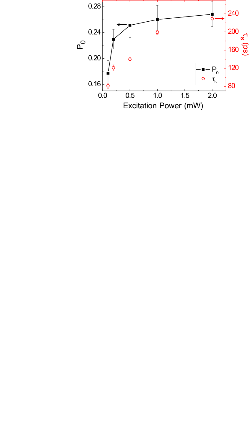
Figure 6: Initial spin polarization $P_{0}$ (black filled squares) and spin lifetime $\tau_{s}$ (red open circles) as a function of excitation power for the $122$ Å wide QW at an excess energy of $176$ meV. The black line is a guide to the eye.

In Sec. III.2 we obtained a qualitative estimate for the initial spin relaxation by evaluating the average spin precession period $T_{z}$ of the optically excited electron states prior to the first scattering event. In a more realistic picture, we must take into account multiple scattering events, too. Each time an electron is scattered from a state with in-plane wave vector $\bm{k}_{\|}$ to a state $\bm{k}_{\|}^{\prime}$, it is exposed to a differently oriented effective magnetic field $\bm{\Omega}(\bm{k}_{\|}^{\prime})$. Frequent momentum scattering events thus reduce the spin relaxation, which is known as motional narrowing. Slichter (1963); Dyakonov and Perel (1972) There are inelastic scattering events such as electron-phonon scattering, as well as elastic momentum scattering events which include, e.g., electron-impurity scattering and electron-electron scattering. While the former processes are approximately independent of the density of excited electrons, electron-electron scattering becomes more efficient with increasing electron density. For low excitation powers, momentum scattering is less efficient so that the initial spin relaxation is hardly reduced by motional narrowing. For the parameters of Fig. 6, we have a very short precession period $T_{z}\approx 2.5$ ps, see Fig. 5. The measured polarization $P_{0}$ is therefore very low due to effective initial spin relaxation. When the excitation power is increased, electron-electron scattering and motional narrowing become more efficient. Therefore, the initial spin relaxation is reduced and the measured spin polarization $P_{0}$ increases with excitation power. All data shown in Fig. 4 was obtained with an excitation power of $1$ mW where initial spin relaxation was partly suppressed by motional narrowing. Of course, electron-electron scattering and motional narrowing affect not only the initial spin relaxation but also the spin relaxation at later times, as described by $\tau_{s}$ in Eq. (3). Consistent with the above arguments, we obtain spin relaxation times $\tau_{s}$ which increase with excitation power, see the open circles in Fig. 6. Finally we note that for the low to moderate excitation powers considered here phase space filling of the exciton states is not important.

IV Theoretical Analysis

IV.1 Theoretical model

Our theory for the excitonic absorption follows Ref. Winkler, 1995. The main idea is to expand the exciton wave functions in terms of electron and hole states. The exciton Schrödinger equation is then solved in momentum space by means of a modified quadrature method. Finally we calculate the energy-dependent absorption coefficient using Fermi’s Golden Rule.

For both the electron and hole states we use an $8\times 8$ Kane multiband Hamiltonian Trebin et al. (1979) containing the lowest conduction band $\Gamma_{6}^{c}$, the topmost valence $\Gamma_{8}^{v}$ and the split-off valence band $\Gamma_{7}^{v}$. In the axial approximation, Winkler (2003) the single-particle states become

$$\psi_{n\bm{k}}(\bm{r})=\frac{1}{2\pi}\sum_{j}e^{i\bm{k}\cdot\bm{\rho}}\;e^{-iM_{j}\varphi}\>\xi^{j}_{nk}(z)\,u_{j}(\bm{r})\;,$$ (7)

where $\bm{r}=(\bm{\rho},z)$ is the position vector and $n$ is the subband index. In this section, $\bm{k}=(k\cos\varphi,k\sin\varphi)$ is the in-plane wave vector, i.e., we omit the index $\|$. The quantum number $M_{j}$ is the $z$ component of the angular momentum of the $j$th spinor component $\xi_{n\bm{k}}^{j}(z)$, i.e., in the $8\times 8$ model used here, $M_{j}$ generalizes the quantum number $S_{z}$ used in the preceding sections of this paper. Finally, $u_{j}(\bm{r})$ are bulk band edge Bloch functions. It is important to note that, due to the sum over $j$, the states (7) are not eigenstates of angular momentum. Only for $\bm{k}=0$ the hole states are pure HH or LH states. We thus label hole subbands as HH or LH-like according to the dominant spinor components at $\bm{k}=0$. Due to HH-LH mixing, we cannot distinguish between these subbands at large wave vectors $k$.

In the following, we consider only the optically active exciton states with center-of-mass momentum zero. Accordingly, the exciton states depend only on the relative coordinate $\bm{\rho}=\bm{\rho}_{e}-\bm{\rho}_{h}$, where the index $e$ ($h$) refers to electron (hole) states. In the axial approximation, the exciton states can be classified by $l$, the $z$ component of the total angular momentum. The exciton states then read

$$\Psi_{l\alpha}(\bm{\rho},z_{e},z_{h})=\frac{1}{(2\pi)^{3/2}}\sum_{n_{e},\,n_{h}}\sum_{j_{e},\,j_{h}}\int d^{2}k\>\phi_{l\alpha\,k}^{n_{e}n_{h}}\>e^{i\bm{k}\cdot\bm{\rho}}\>e^{i(l-M_{j_{e}}+M_{j_{h}})\varphi}\>\xi^{j_{e}}_{n_{e}k}(z_{e})\;\xi^{j_{h}\,\ast}_{n_{h}k}(z_{h})\;u_{j_{e}}(\bm{r})\,u_{j_{h}}^{\ast}(\bm{r})\,,$$ (8)

where $\phi_{l\alpha\,k}^{n_{e}n_{h}}$ are the expansion coefficients. The index $\alpha$ labels exciton states with the same value of $l$. Unlike the exciton states in simplified theories (see, e.g., Ref. Maialle et al., 1993), the exciton states (8) cannot be written as a direct product of electron and hole states with well-defined quantum numbers of angular momentum. In Eq. (8) only $l$ and $\alpha$ are good quantum numbers.

Using Fermi’s Golden Rule, the oscillator strength of the excitons per unit area is given by

$$f_{l\alpha}^{\,\hat{\bm{e}}}=\frac{1}{\pi\,m_{0}\,E_{l\alpha}}\;\bigg{|}\sum_{n_{e},\,n_{h}}\sum_{j_{e},\,j_{h}}\mathcal{P}_{l\alpha\,n_{e}n_{h}}^{j_{e}j_{h}}\bigg{|}^{2}\;,$$ (9a)

where $$E_{l\alpha} (l,\alpha)$$ is the energy of the exciton , and the components of the dipole matrix elements are

$$\mathcal{P}_{l\alpha\,n_{e}n_{h}}^{j_{e}j_{h}}=\delta_{l-M_{j_{e}}+M_{j_{h}},\,0}\;\int dk\,k\;\phi_{l\alpha\,k}^{n_{e}n_{h}}\>\int dz\;\xi^{j_{h}\,\ast}_{n_{h}k}(z)\>\xi^{j_{e}}_{n_{e}k}(z)\>\langle u_{j_{h}}|\,\hat{\bm{e}}\cdot\bm{p}\,|u_{j_{e}}\rangle\,.$$ (9b)

Here, $\bm{p}$ is the momentum operator and $\hat{\bm{e}}$ denotes the polarization vector of the incident light. We have $\hat{\bm{e}}=(1/\sqrt{2})(1,\pm i,0)$ for $\sigma^{\pm}$ polarized light. The matrix elements $\langle u_{j_{h}}|\,\bm{p}\,|u_{j_{e}}\rangle$ are the same as those momentum matrix elements in the $8\times 8$ Kane Hamiltonian which are responsible for the off-diagonal $\bm{k}\cdot\bm{p}$ coupling between conduction and valence bands. In our theoretical model, Eq. (9) replaces the selection rules depicted in Fig. 1. The Kronecker $\delta$ in Eq. (9b) is reminescent of the simple selection rules. For circularly polarized light (polarization $\sigma^{\pm}$) only excitons with $l=\pm 1$ are optically active.

The absorption spectrum is given by

$$\alpha_{\hat{\bm{e}}}\,(\omega)=\alpha_{0}\>\sum_{l,\alpha}f_{l\alpha}^{\,\hat{\bm{e}}}\>\delta(\hbar\omega-E_{l\alpha})\,,$$ (10)

where $\alpha_{0}=\hbar e^{2}\pi/(2m_{0}\varepsilon_{0}cn)$ with $n$ the index of refraction and $\hbar\omega$ is the excitation energy. In the numerical calculations we replace the delta functions by a phenomenological Lorentzian broadening.

The electron spin orientation induced by the optical creation of an exciton $(l,\alpha)$ is the expectation value of the electron spin operator $\hat{S}_{z}^{e}$

$$M_{l\alpha}^{e} = \langle\hat{S}_{z}^{e}\rangle_{l\alpha}$$

$$= \sum_{j_{e}}M_{j_{e}}\!\sum_{n_{e},\,n_{h}}\int dk\,k\;\big{|}\phi_{l\alpha\,k}^{n_{e}n_{h}}\big{|}^{2}\int dz_{e}\;\big{|}\xi^{j_{e}}_{n_{e}k}(z_{e})\big{|}^{2}\,.$$

The number of optically excited excitons $(l,\alpha)$ is proportional to the oscillator strength $f_{l\alpha}^{\,\hat{\bm{e}}}$. Accordingly, the spin polarization $S_{e}(\omega)$ of the electron systems is given by

$$S_{e}(\omega)=\frac{\alpha_{0}}{\alpha_{\hat{\bm{e}}}\,(\omega)}\sum_{l,\alpha}M_{l\alpha}^{e}\,f_{l\alpha}^{\,\hat{\bm{e}}}\>\delta(\hbar\omega-E_{l\alpha})\,.$$ (12)

It is the quantity $S_{e}(\omega)$ which we compare with the measured spin polarization $P_{0}$.

IV.2 Discussion

In Sect. III we demonstrated the good agreement between the measured data and the calculated spin polarization. In this section we will show that a detailed understanding of these results can be achieved based on a careful examination of the calculated spectra.

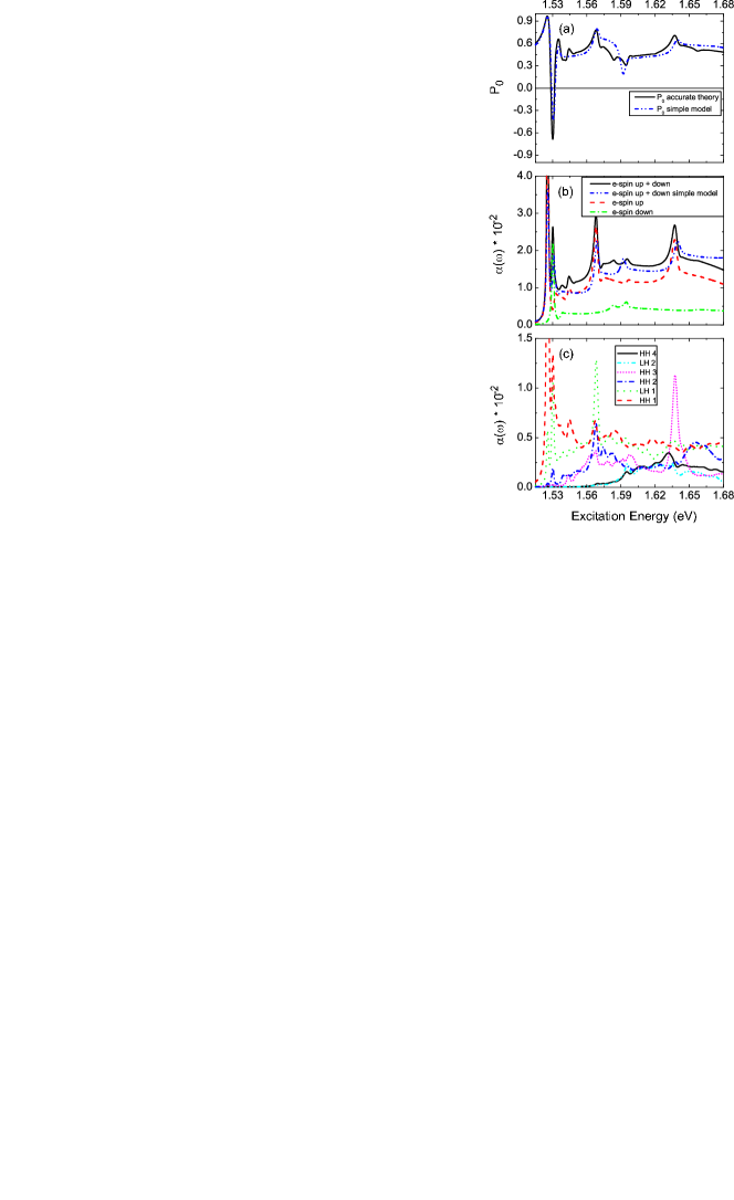
Figure 7: Calculated initial degree of polarization $P_{0}$ and absorption coefficient $\alpha(\omega)$ for circularly polarized light as a function of excitation energy for the 198 Å wide GaAs/AlAs QW. The black lines in (a) and (b) show $P_{0}$ and $\alpha(\omega)$ for the full theory, whereas the dashed-double-dotted lines show for comparison the results for a simplified model that neglects valence band mixing and HH-LH coupling. The red dashed line (green dash-dotted line) in (b) shows the partial absorption spectra for spin up (spin down) electrons. Panel (c) displays the hole subband contributions (13) to $\alpha(\omega)$ for the full theory.

As an example, we show in Fig. 7(a) the calculated electron spin polarization $S_{e}(\omega)$ and in Fig. 7(b) the absorption coefficient $\alpha(\omega)$ for the $198$ Å wide QW, see also Fig. 3. Frequently the interpretation of excitonic spectra is based on the simple and intuitive idea that the excitons giving rise to the peaks in the spectra can be attributed to pairs of individual electron and hole subbands. However, such a scheme must be used with caution because the spectra are often strongly affected by valence band mixing and Coulomb coupling between subbands. Winkler (1995) To illustrate the importance of these effects, the dashed-double-dotted lines in Figs. 7(a) and 7(b) show the results of a simplified calculation that neglects these couplings. Both the absorption coefficient and the initial spin polarization differ remarkably in these models. In particular, we find that the oscillator strength of the HH3:E1(1s) exciton is by a factor $\sim 50$ smaller if these couplings are neglected so that the peak cannot be resolved on the scale of Fig. 7. Furthermore, the peaks labeled HH2:E2(1s) and HH3:E3(1s) are shifted to higher energies.

In order to quantify the valence band mixing, we can evaluate the contribution of different hole subbands to the oscillator strengths $f_{l\alpha}^{\,\hat{\bm{e}}}$. We define the partial oscillator strengths

$$f_{l\alpha,n_{h}}^{\,\hat{\bm{e}}}=\frac{1}{\mathcal{N}}\,\bigg{|}\sum_{n_{e}}\sum_{j_{e},\,j_{h}}\mathcal{P}_{l\alpha\,n_{e}n_{h}}^{j_{e}j_{h}}\bigg{|}^{2}\;,$$ (13a)

where the normalization $$\mathcal{N}$$ is chosen such that we have

$$\sum_{n_{h}}f_{l\alpha,n_{h}}^{\,\hat{\bm{e}}}=f_{l\alpha}^{\,\hat{\bm{e}}}\;.$$ (13b)

Similar to Eq. (10) we then calculate partial spectra showing the contributions of each hole subband to the absorption coefficient, see Fig. 7(c). The complicated curves clearly illustrate that the labeling in terms of subbands is very problematic. For example, the contribution of the HH1 subband to the oscillator strength of the LH1:E1(1s) exciton is larger than the contribution of the LH1 subband. For comparison, we show in Fig. 8 the hole subband dispersion curves of the 198 Å wide QW.

Figure 8: Hole subband dispersion curves calculated for the 198 Å wide QW.

We suggest here a different approach for decomposing the spectra that yields a much clearer physical picture. We can identify whether the oscillator strength of an exciton is predominantly from the dipole matrix element (9b) between a hole and a spin-up or a spin-down electron state by evaluating the partial oscillator strengths

$$f_{l\alpha,j_{e}}^{\,\hat{\bm{e}}}=\frac{1}{\mathcal{N}}\,\bigg{|}\sum_{n_{e},\,n_{h}}\sum_{j_{h}}\mathcal{P}_{l\alpha\,n_{e}n_{h}}^{j_{e}j_{h}}\bigg{|}^{2}\;,$$ (14)

where the normalization $\mathcal{N}$ is choosen analogously to Eq. (13b). We then calculate partial spectra for the spin-up and spin-down spinor components $j_{e}$, see the dashed and dash-dotted lines in Fig. 7(b). For the different QWs investigated in this work, we show the partial oscillator strengths (14) in the bottom panels of Figs. 3 and 4.

For the eight-component spinors (7) we obtain eight partial oscillator strengths (14). However, for the electron states, the contributions of the valence band spinor components are very small so that they could not be resolved using the scale of Fig. 7. (Yet these spinor components are very important for the correct absolute values of the exciton energies. Winkler (1995)) The partial oscillator strengths $f_{l\alpha,j_{e}}^{\,\hat{\bm{e}}}$ for the spin-up and spin-down components of the electron states are essentially equivalent to the corresponding partial oscillator strengths $f_{l\alpha,j_{h}}^{\,\hat{\bm{e}}}$ of the HH and LH components of the hole states, see Fig. 1. These partial oscillator strengths would be strictly equal in a $6\times 6$ model that neglects the split-off valence band $\Gamma_{7}^{v}$.

Unlike for the partial oscillator strengths (13), we get from Eq. (14) a clear and simple decomposition of the spectra. In particular, a comparison between the partial spectra in Fig. 7(b) and the electron spin polarization in Fig. 7(a) shows that each resonance can be labeled as an excitation of either spin-up or spin-down electrons, consistent with Fig. 1. In spite of the strong admixture of different hole subbands visible in Fig. 7(c) it is either the electron spin-up or the spin-down component (i.e., the HH or the LH component) of an exciton that is optically active. The reason why we get much clearer results from Eq. (14) than from Eq. (13) lies in the fact that the labeling of hole subbands as HH- or LH-like (see Fig. 8) is not rigorously justified, but it reflects merely the dominant spinor component around $k=0$. For larger in-plane wave vectors, the subbands are strongly affected by HH-LH mixing. Yet the excitons (8) “try to avoid the HH-LH mixing by selecting the spinor components as a function of $k$ from different hole subbands.” This is also the reason why we can label most of the excitonic resonances by pairs of electron and hole subbands (Fig. 3). This scheme refers to the pairs of electron and hole subbands that contribute the largest around $k=0$. At larger wave vectors $k$ in the expansion (8), the exciton states contain large contributions from other subbands, too.

In spite of the fact that we can label the excitonic resonances by pairs of electron and hole subbands, the oscillator strengths of the individual resonances in Fig. 7(b) are very different from those in Fig. 1. To illustrate this point, Fig. 9(a) shows the oscillator strength of the HH1:E1(1s) and the LH1:E1(1s) exciton as a function of well width while Fig. 9(b) shows the ratio between these quantities. Only in the limit of very wide QWs we approach the bulk value 3. The ratio decreases with decreasing well width due to HH-LH coupling. For energies larger than the HH1:E1 absorption edge ($E>1.535$ eV for the $198$ Å wide QW), the individual peaks in the spectra are Fano resonances, i.e., they are degenerate with the continua of excitons from lower subband pairs. The peaks on top of the continua are thus less important for the electron spin polarization observed at these energies. The magnitude of the electron spin polarization in this regime is always smaller than one.

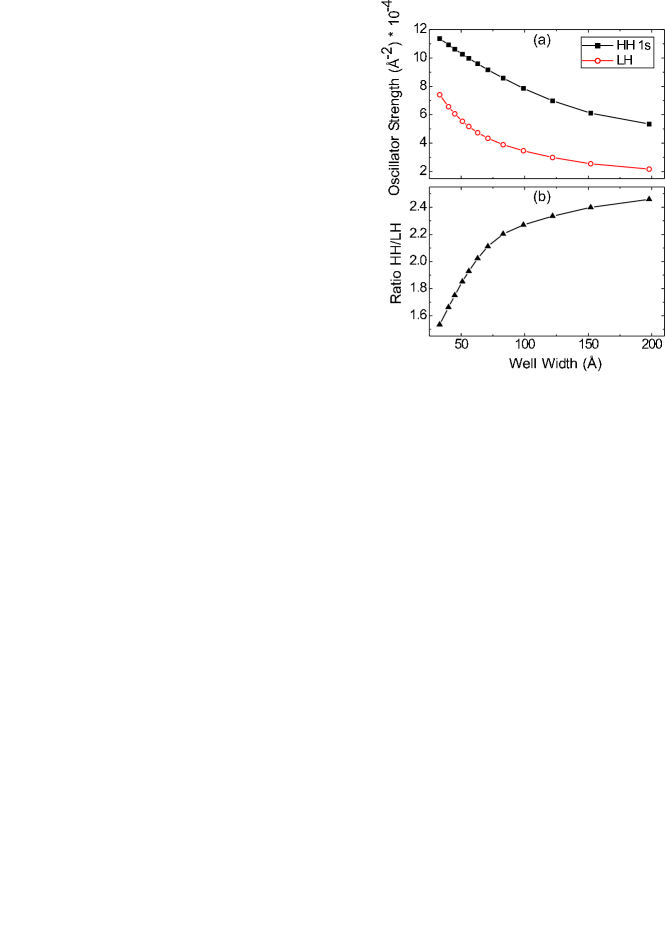
Figure 9: Calculated oscillator strength (a) for the HH and LH transitions as a function of the QW width. The ratio between the HH and LH oscillator strength is shown in (b).

The good agreement between the theory and the experimental data has been demonstrated in Figs. 3 and 4. It indicates that our basic assumption $P_{\mathrm{opt}}=P_{s}$ is justified. This implies that the orientation of the electron spins is essentially preserved when the electrons relax from the optically excited high-energy states to a thermal equilibrium for their momentum distribution. (Only in narrow QWs the measured optical polarization is smaller than the calculated electron spin polarization due to initial spin relaxation.)

At a first glance, our findings suggest that in our experiments electrons and holes relax independently from the optically excited state to quasi-thermal equilibrium, the reason being that in a single-particle picture the spin of the electrons is a good quantum number. alm On the other hand, only excitons with angular momentum quantum number $l=\pm 1$ can absorb or emit photons with polarization $\sigma^{\pm}$. With $\sigma^{+}$ polarized light we thus excite only excitons with angular momentum $l=+1$. If the excitons preserved the angular momentum quantum number $l$ while they relax from the optically excited states to thermal equilibrium, the measured optical polarization $P_{\mathrm{opt}}$ would be the same like the polarization of the exciting laser beam, independent of the energy of the laser. This disagrees clearly with our experimental findings. We note, however, that each dublet of optically active excitons with $l=\pm 1$ is almost degenerate with a dublet of optically inactive excitons with $l=\pm 2$ or $l=0$ (Refs. Winkler, 1995; exc, ). The latter dublet is related to the optically active excitons by a spin flip of the hole. The electron spin of the exciton state (but not $l$) can thus be preserved even if the hole spin of the exciton is flipped. Therefore, we cannot decide, based on our experiments whether electrons and holes relax independently or whether they relax as a Coulomb-correlated exciton state. Recently, two groups were able to gain information on exciton formation dynamics in GaAs quantum wells by using optical-pump THz-probe spectroscopy and time-resolved PL on a very high quality quantum well.Kaindl et al. (2003); Szczytko et al. (2004)

V Conclusions

Using time resolved photoluminescence excitation spectroscopy and a multiband envelope function theory of excitonic absorption based on the $8\times 8$ Kane Hamiltonian, we have studied the energy dependence of the initial degree of spin polarization of optically created electrons in GaAs QWs with different well widths. Taking into account Coulomb coupling and HH-LH coupling between subbands was shown to be essential to obtain good agreement between theory and experiment for a wide range of excitation energies. The calculated results differ significantly from the experimental data if a frequently used simplified exciton model is applied that neglects these couplings. This work therefore provides the first quantitative picture of the optical orientation of electron spins in GaAs QWs.

The good agreement between the measured degree of optical polarization $P_{\mathrm{opt}}$ and the calculated spin polarization $P_{s}$ of the electrons indicates that our basic assumption $P_{\mathrm{opt}}=P_{s}$ is justified. This implies that the orientation of the electron spins is (essentially) preserved when the electrons relax from the optically excited high-energy states to a thermal equilibrium for their momentum distribution. In narrow QWs the measured optical polarization is smaller than the calculated electron spin polarization due to initial spin relaxation. However, this process is found to be essentially independent of the energy of the exciting photons. Initial spin relaxation is most effective for small excitation powers. For larger excitation powers it becomes less important because of motional narrowing.