Stationary states and energy cascades in inelastic gases

Abstract

We find a general class of nontrivial stationary states in inelastic gases where, due to dissipation, energy is transfered from large velocity scales to small velocity scales. These steady-states exist for arbitrary collision rules and arbitrary dimension. Their signature is a stationary velocity distribution $f(v)$ with an algebraic high-energy tail, $f(v)\sim v^{-\sigma}$. The exponent $\sigma$ is obtained analytically and it varies continuously with the spatial dimension, the homogeneity index characterizing the collision rate, and the restitution coefficient. We observe these stationary states in numerical simulations in which energy is injected into the system by infrequently boosting particles to high velocities. We propose that these states may be realized experimentally in driven granular systems.

Energy dissipation has profound consequences in granular media. It is responsible for collective phenomena such as hydrodynamic instabilities gz ; km , shocks rbss ; slk ; bcdr , and clustering my ; ou ; mwl . The inelastic nature of the collisions remains crucially important in dilute settings and under vigorous forcing where, in contrast with molecular gases, there is no energy equipartition wp ; fm and the velocity distributions are typically non-Maxwellian kwg ; ep ; ve ; rm ; ao ; bbrtv . In this letter, we show that energy dissipation also results in self-sustaining stationary states where energy cascades from large velocity scales to small velocity scales, and we propose that these states may be realized experimentally in driven granular gases.

Hydrodynamic theory of granular flows is formulated using inelastic gases as a starting point pkh ; jr ; gzb ; bdks ; ig . Without forcing, dissipation is quantified via the energy balance equation, $dT/dt=-\Gamma$, where $T=\langle v^{2}\rangle$ is the temperature and $\Gamma$ the dissipation rate. Collisions involving a pair of particles with relative velocity $\Delta v$ occur with rate $\propto(\Delta v)^{\lambda}$ and result in energy loss $\propto(\Delta v)^{2}$. Assuming that a single velocity scale characterizes the system, $\Gamma\sim\langle(\Delta v)^{2+\lambda}\rangle\sim T^{1+\lambda/2}$, leads to Haff’s cooling law, $T\sim t^{-2/\lambda}$ (exponential decay occurs when $\lambda=0$). Hence, the temperature decays indefinitely and the velocity distribution $f(v)$ approaches the trivial steady-state $f(v)\to\delta(v)$ where all particles are at rest, a stationary state that can be considered as a dynamical fixed point. However, the energy balance equation assumes a finite dissipation rate. This need not be the case!

Our main result is that there is a general class of nontrivial stationary states where the velocity distribution has an algebraic high-energy tail

$$f(v)\sim v^{-\sigma}$$ (1)

as $v\to\infty$. First, we obtain this result in one-dimension and then, generalize it to arbitrary dimension.

Our system is an ensemble of identical particles that undergo inelastic collisions

$$v_{1,2}=pu_{1,2}+qu_{2,1}$$ (2)

with $u_{1,2}$ ($v_{1,2}$) the pre-collision (post-collision) velocities. The collision parameters $p$ and $q$ obey $p+q=1$ so momentum is conserved. In each collision, the relative velocity is reduced by the restitution coefficient $r=1-2p$ and the energy loss equals $pq(u_{1}-u_{2})^{2}$. We consider general collision rates $|u_{1}-u_{2}|^{\lambda}$ with $\lambda$ the homogeneity index. For particles interacting via the central potential $U(r)\sim r^{-a}$ then $\lambda=1-2\frac{d-1}{a}$ so $\lambda\leq 1$ rd . Hard-spheres, $\lambda=1$, model ordinary granular media. Maxwell molecules mhe , $\lambda=0$, model granular particles with dipole interactions, such as magnetic particles or particles immersed in a fluid ia .

We seek stationary velocity distributions $f(v)$ that obey the Boltzmann equation

$$\iint du_{1}\,du_{2}\,|u_{1}-u_{2}|^{\lambda}\,f(u_{1})f(u_{2})\qquad\qquad\qquad$$ (3)

$$\times\left[\delta(v-pu_{1}-qu_{2})-\delta(v-u_{1})\right]=0,$$

reflecting balance of gain and loss due to collisions.

The case $\lambda=0$ is instructive as the velocity distribution can be obtained explicitly. The Boltzmann equation is a simple convolution because the collision rate is constant, and it is conveniently studied using the Fourier transform $F(k)=\int dv\,f(v)\,e^{ikv}$ that satisfies the nonlinear, nonlocal equation $F(k)=F(pk)F(qk)$. Normalization implies $F(0)=1$. For elastic collisions ($p=0$) any distribution is stationary, but this is just a one-dimensional pathology. Generally, for any value of the restitution coefficient, there is a family of solutions $F(k)=\exp\big{(}-v_{0}|k|\big{)}$ with arbitrary typical velocity $v_{0}$. As a result, the velocity distribution is Lorentzian

$$f(v)=\frac{1}{\pi v_{0}}\frac{1}{1+(v/v_{0})^{2}}.$$ (4)

We note that this distribution is independent of the restitution coefficient. The typical velocity $v_{0}$ is finite, but the average energy is infinite.

This distribution does not evolve under the inelastic collision dynamics and in particular, the energy density remains constant. From the energy balance equation, one might have expected that the velocity distribution constantly narrows because particles dissipate energy, but quite surprisingly, the heavy tail of the velocity distribution acts as a heat bath, balancing the energy dissipation and maintaining a steady velocity distribution. We conclude that, in addition to the trivial state where all particles are at rest, there is another fixed point, a self-sustaining stationary state.

For general collision rules, the characteristic exponent $\sigma$ can be found analytically. For large $v$, the convolution in Eq. (3) is governed by the product $f(u_{1})f(u_{2})$ with one of the pre-collision velocities large and the other small because the distribution decays sharply at large velocities. The Boltzmann equation includes a loss term and a gain term. For the loss term, $u_{1}=v$ is large and $u_{2}$ is small. For the gain term, there are two separate contributions. Either $v=pu_{1}$ and then $u_{2}$ is small or $v=qu_{2}$ and then $u_{1}$ is small. In either case, the double integral separates. The integral over the smaller velocity equals one. With the remaining integral over the larger velocity, denoted by $u$, the nonlinear Boltzmann equation becomes linear for large $v$

$$\int\!du\,|u|^{\lambda}f(u)\left[\delta(v\!-\!pu)\!+\!\delta(v\!-\!qu)\!-\!\delta(v\!-\!u)\right]=0.\quad$$ (5)

Consequently, the tail of the distribution satisfies the functional equation

$$\frac{1}{p^{1+\lambda}}f\left(\frac{v}{p}\right)+\frac{1}{q^{1+\lambda}}f\left(\frac{v}{q}\right)-f(v)=0$$ (6)

describing cascade of energy from large velocities to small ones, $v\to(pv,qv)$. The power-law decay (1) satisfies this equation when $p^{\sigma-1-\lambda}+q^{\sigma-1-\lambda}=1$, and since $p+q=1$, the characteristic exponent is

$$\sigma=2+\lambda.$$ (7)

In one-dimension, $\sigma$ is independent of the restitution coefficient.

We comment that the full nonlinear Boltzmann equation assumes molecular chaos as the two-particle velocity distribution is a product of one-particle distributions. However, the equation governing the tail is linear and it is valid under less stringent conditions. The only requirement is that energetic particles are weakly correlated with slower ones.

In arbitrary dimension $d$, the collision law is

$${\bf v}_{1}={\bf u}_{1}-(1-p)({\bf u}_{1}-{\bf u}_{2})\!\cdot\!\hat{\bf n}\,\hat{\bf n}.$$ (8)

Momentum transfer occurs only along the normal direction with $\hat{\bf n}$ a unit vector parallel to the impact direction connecting the particles. The energy dissipation equals $p(1-p)|({\bf u}_{1}-{\bf u}_{2})\!\cdot\!\hat{\bf n}|^{2}$ and the collision rate is $|({\bf u}_{1}-{\bf u}_{2})\!\cdot\!\hat{\bf n}|^{\lambda}$.

We derive the linear equation governing the tail of the distribution directly from the collision rule. With the large velocity ${\bf u}$, its magnitude $u\equiv|{\bf u}|$ and $\mu=(\hat{\bf u}\cdot\hat{\bf n})^{2}$, the collision rate is $u^{\lambda}\mu^{\lambda/2}$. The cascade process is $v\to(\alpha v,\beta v)$ with the stretching parameters $\alpha=(1-p)\mu^{1/2}$ and $\beta=[1-(1-p^{2})\mu]^{1/2}$ for ${\bf v}=(1-p){\bf u}\cdot\hat{\bf n}\,\hat{\bf n}$ and ${\bf v}={\bf u}-(1-p){\bf u}\cdot\hat{\bf n}\,\hat{\bf n}$, respectively beta . Integrating over the impact angle $\hat{\bf n}$ and the velocity magnitude $u$, Eq. (5) generalizes as follows

$$\left<\int\!du\,u^{\lambda+d-1}\!f(u)\!\left[\delta(v\!-\!\alpha u)\!+\!\delta(v\!-\!\beta u)\!-\!f(v)\right]\!\mu^{\lambda/2}\!\!\right>\!=\!0.$$

Here, the brackets are used as shorthand for the angular integration, $\langle g\rangle=\int d\hat{\bf n}\,g(\hat{\bf n})$. Integrating over $u$ yields

$$\left<\left[\frac{1}{\alpha^{d+\lambda}}f\left(\frac{v}{\alpha}\right)+\frac{1}{\beta^{d+\lambda}}f\left(\frac{v}{\beta}\right)-f(v)\right]\!\mu^{\lambda/2}\!\right>=0.\quad$$ (9)

The power-law decay (1) satisfies this equation provided that the exponent $\sigma$ is root of the equation $\left<\left(1-\alpha^{\sigma-d-\lambda}-\beta^{\sigma-d-\lambda}\right)\mu^{\lambda/2}\right>=0$. The angular integration is performed using spherical coordinates. Given $\mu=\cos^{2}\theta$, then $d\hat{\bf n}\propto(\sin\theta)^{d-2}d\theta$, and $\langle\,g\,\rangle\propto\int_{0}^{1}d\mu\,\mu^{-{1\over 2}}(1-\mu)^{d-3\over 2}g(\mu)$. The equality for the exponent $\sigma$ can be written in terms of the gamma function and the hypergeometric function gr

$$\frac{1\!-\!{}_{2}F_{1}\!\left(\frac{d+\lambda-\sigma}{2},\frac{\lambda+1}{2},\frac{d+\lambda}{2},1\!-\!p^{2}\right)}{(1-p)^{\sigma-d-\lambda}}\!=\!\frac{\Gamma(\frac{\sigma-d+1}{2})\Gamma(\frac{d+\lambda}{2})}{\Gamma(\frac{\sigma}{2})\Gamma(\frac{\lambda+1}{2})}.\quad$$ (10)

In the cascade process $v\to(\alpha v,\beta v)$, the total velocity magnitude increases ($\alpha+\beta\geq 1$) even though the total energy decreases ($\alpha^{2}+\beta^{2}\leq 1$). Utilizing these inequalities, we deduce the bounds $1\leq\sigma-d-\lambda\leq 2$ from the embedded equation for the characteristic exponent. The lower bound (7) is realized in one-dimension where collisions are head-on ($\mu=1$). The upper bound is approached, $\sigma\to d+2+\lambda$, in the quasi-elastic limit, $r\to 1$. This, combined with the known Maxwellian distribution that occurs for elastic collisions, demonstrates the singular nature of the quasi-elastic limit. Interestingly, the energy may be either finite or infinite, depending on whether $\sigma$ is larger or smaller than $d+2$. In either case, the integral underlying the dissipation rate is divergent, a general characteristic of the stationary distributions.

Generally, the exponent $\sigma$ increases monotonically with the spatial dimension $d$, the homogeneity index $\lambda$, and the restitution coefficient $r$. For completely inelastic ($r=0$) hard spheres, we find $\sigma=4.14922$ and $\sigma=5.23365$ for $d=2$, $3$, respectively. The exponents for completely inelastic Maxwell molecules are $\sigma=3.19520$ and $\sigma=4.28807$ for $d=2$, $3$. These values provide lower bounds on $\sigma$ with respect to $r$, as shown in figure 1.

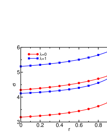
Figure 1: The exponent $\sigma$ as a function of the restitution coefficient $r$ for $\lambda=0$ (circles) and $\lambda=1$ (squares). The lower curves correspond to $d=2$ and the upper to $d=3$.

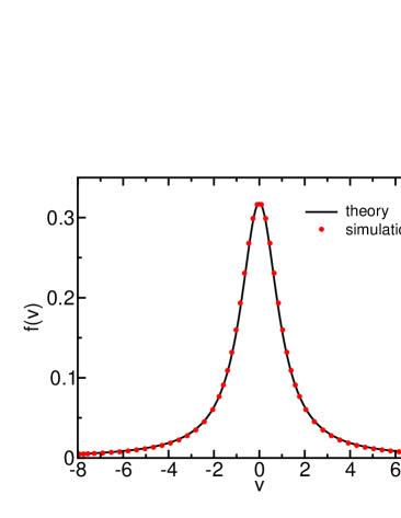
Figure 2: The velocity distribution $f(v)$ versus $v$ for Maxwell molecules in one-dimension. The velocity was rescaled to compare with an ordinary Lorentzian.

A remarkable feature is that the characteristic exponent changes continuously with the parameters $d$, $\lambda$, and $r$. Hence, the tails are not universal. The power-law decay stands in contrast with the stretched exponentials, $f(v)\sim\exp(-v^{\nu})$, with $\nu=\lambda$ and $\nu=1+\lambda/2$, respectively, for unforced and thermally forced inelastic gases ep ; ve ; rm ; ao . Previously, algebraic tails with different exponents were found but for non-stationary distributions describing freely cooling Maxwell molecules bk ; bmp ; eb .

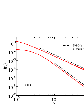
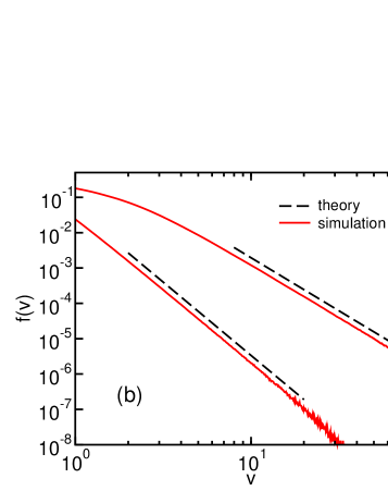
Figure 3: The velocity distribution $f(v)$ versus $v$ for Maxwell molecules (a) and hard spheres (b) in one-dimension (upper lines) and two-dimension (lower lines). The theoretical prediction is shown for reference.

These steady-state distributions can be realized, up to some cutoff, in finite systems of driven inelastic particles. The key is to inject energy at a very large velocity scale. Numerically, we used the following simulation. Initially, we start with an innocuous velocity distribution, uniform with support in $[-1:1]$. Particles collide inelastically, and an energy loss “counter” keeps track of the aggregate energy loss. With rate $\gamma$, small compared with the collision rate, a particle is selected at random and it is energized by an amount equal to the aggregate energy loss. Subsequently, the energy loss counter is reset to zero. The rationale behind this simulation is that the total energy remains practically constant and more importantly, that energy is injected only at the tail of the distribution. In effect, this procedure does not alter the purely dissipative dynamics, except for setting a scale for the most energetic particles.

We simulated completely inelastic hard-spheres and Maxwell molecules in one- and two-dimensions. We used $N=10^{7}$ ($N=10^{5}$) particles and injection rate $\gamma=10^{-4}$ ($\gamma=10^{-2}$) for $\lambda=0$ ($\lambda=1$). We verified that: (i) after a transient, the velocity distribution becomes stationary, (ii) the velocity distribution is Lorentzian for one-dimensional Maxwell molecules (figure 2), (iii) the velocity distribution has an algebraic tail, and (iv) $\sigma$ is consistent with theory (figure 3).

The very same stationary distributions can be reached using other simulation methods. For example, particles may be re-energized such that their velocity is drawn from a Maxwellian distribution with a typical energy proportional to the system size (the data presented for one-dimensional hard-spheres are from such a simulation). We conclude that the simulations confirm the existence of the nontrivial stationary states with power-law tails. These steady-states are stable fixed points as the system is driven into them even when starting from compact distributions. Moreover, stability analysis of the time dependent version of Eq. (9) shows that the stationary distribution (1) is stable with respect to perturbations consisting of steeper algebraic tails.

Clearly, if $f(v)$ is a steady-state so is $v_{0}^{-d}f(v/v_{0})$ for an arbitrary typical velocity $v_{0}$. The injection protocol selects $v_{0}$. Suppose that particles are boosted at rate $\gamma$ per particle to velocity $V$, a scale that sets an upper cutoff on the velocity distribution finite . The energy injection rate is $\gamma V^{2}$, and the energy dissipation rate is $\Gamma\sim\langle v^{2+\lambda}\rangle$ with $\langle g\rangle\equiv\int^{V}dv\,v^{d-1}f(v)g(v)$. Energy balance, $\Gamma\sim\gamma V^{2}$, relates the injection rate, the injection scale, and the typical velocity scale, $\gamma\sim V^{\lambda}(V/v_{0})^{d-\sigma}$.

In our simulations, energy is maintained constant, $\langle v^{2}\rangle\sim 1$. When $\sigma<d+2$, the constant energy constraint implies $V^{d+2-\sigma}\sim v_{0}^{d-\sigma}$, that combined with energy balance reveals how the maximal velocity, $V\sim\gamma^{-1/(2-\lambda)}$, and the typical velocity, $v_{0}\sim\gamma^{\frac{d+2-\sigma}{(\sigma-d)(2-\lambda)}}$, scale with the injection rate. When $\sigma>d+2$, the initial conditions set the typical velocity: $\langle v^{2}\rangle\sim v_{0}^{2}$ implies $v_{0}\sim 1$, and energy balance yields $V\sim\gamma^{-1/(\sigma-d-\lambda)}$. The simulations are consistent with these scaling laws. For example, $V\approx 10^{2}$ and $v_{0}\approx 10^{-2}$ for one-dimensional Maxwell-molecule simulations with $\gamma=10^{-4}$. This, combined with the simulations, demonstrates that finite energy and infinite energy cases differ quantitatively but not qualitatively.

In conclusion, we have shown that inelastic gases have nontrivial stationary states where the velocity distribution has an algebraic high-energy tail. These steady-states are generic in that they exist for arbitrary collision rates, arbitrary collision rules, and arbitrary spatial dimensions. Typically, energy is injected at large velocity scales, and it is dissipated over a range of smaller velocities. Qualitatively, this energy cascade picture is analogous to fluid turbulence. However, without energy conservation, there is an important difference with the conventional Kolmogorov spectra: the characteristic exponents are not universal and they do not follow from dimensional analysis zlf .

In an infinite system, there is perfect balance between collisional loss and gain and the high-energy tail enables the stationary state, while in finite systems, energy injection maintains the steady-state. The latter is relevant to granular gas experiments that are typically performed in steady-state conditions. We propose that stable distributions and energy cascades may be realized using an experimental set-up in which energy is added at large velocity scales via rare but powerful energy injections.

We thank A. Baldassarri, N. Menon, and H. A. Rose for useful discussions. We acknowledge DOE W-7405-ENG-36 and NSF DMR-0242402 for support of this work.

References

- (1) I. Goldhirsch, and G. Zanetti, Phys. Rev. Lett. 70, 1619 (1993).
- (2) E. Khain and B. Meerson, Europhys. Lett. 65, 193 (2004).
- (3) E. C. Rericha, C. Bizon, M. D. Shattuck, and H. L. Swinney, Phys. Rev. Lett. 88, 014302 (2002).
- (4) A. Samadani, L. Mahadevan, and A. Kudrolli, J. Fluid Mech. 452, 293 (2002).
- (5) E. Ben-Naim, S. Y. Chen, G. D. Doolen, and S. Redner, Phys. Rev. Lett. 83, 4069 (1999).
- (6) S. McNamara and W. R. Young, Phys Fluids A 4, 496 (1992).
- (7) J. S. Olafsen and J. S. Urbach, Phys. Rev. Lett. 81, 4369 (1998).
- (8) D. van der Meer, K. van der Weele, and D. Lohse, Phys. Rev. Lett 88, 174302 (2002).
- (9) R. D. Wildman and D. J. Parker, Phys. Rev. Lett. 88, 064301 (2002).
- (10) K. Feitosa and N. Menon, Phys. Rev. Lett. 88, 198301 (2002).
- (11) A. Kudrolli, M. Wolpert, and J. P. Gollub, Phys. Rev. Lett. 78, 1383 (1997).
- (12) S. E. Esipov and T. Pöschel, J. Stat. Phys. 86, 1385 (1997).
- (13) T. P. C. van Noije and M. H. Ernst, Gran. Matt. 1, 57 (1998).
- (14) F. Rouyer and N. Menon, Phys. Rev. Lett. 85, 3676 (2000)
- (15) I. S. Aranson and J. S. Olafsen Phys. Rev. E 66, 061302 (2002).
- (16) A. Barrat, T. Biben, Z. Rácz, E. Trizac, and F. van Wijland, J. Phys. A 35, 463 (2002).
- (17) P. K. Haff, J. Fluid Mech. 134, 401 (1983).
- (18) J. T. Jenkins and M. W. Richman, Phys. Fluids 28, 3485 (1985).
- (19) E. L. Grossman, T. Zhou, and E. Ben-Naim, Phys. Rev. E 55, 4200 (1997).
- (20) J. J. Brey, J. W. Dufty, C. S. Kim, and A. Santos, Phys. Rev. E 58, 4638 (1998).
- (21) I. Goldhirsch, Ann. Rev. Fluid. Mech. 35, 267 (2003).
- (22) P. Résibois and M. de Leener, Classical Kinetic Theory of Fluids (John Wiley, New York, 1977).
- (23) M. H. Ernst, Phys. Reports 78, 1 (1981).
- (24) I. S. Aranson, private communication.
- (25) The parameter is obtained by writing and employing the collision rule, and then using .
- (26) I. S. Gradshteyn and I. M. Ryzhik, Table of Integrals, Series, and Products, (Academic Press, New York, 1972).
- (27) E. Ben-Naim and P. L. Krapivsky, Phys. Rev. E 61, R5 (2000); P. L. Krapivsky and E. Ben-Naim, J. Phys. A 35, L147 (2002).
- (28) A. Baldassarri, U. M. B. Marconi, and A. Puglisi, Europhys. Lett. 58, 14 (2002).
- (29) M. H. Ernst and R. Brito, Europhys. Lett. 58, 182 (2002).
- (30) The system size must be large enough so that finite size scaling effects play no role.
- (31) V. Zakharov, V. Lvov, and G. Falkovich, Kolmogorv Spectra of Turbulence (Springer-Verlag, Berlin, 1992).