Resonating Valence Bond wave function: from lattice models to realistic systems

Abstract

Although mean field theories have been very successful to predict a wide range of properties for solids, the discovery of high temperature superconductivity in cuprates supported the idea that strongly correlated materials cannot be qualitatively described by a mean field approach. After the original proposal by Anderson [P. W. Anderson, Science 235, 1196 (1987)], there is now a large amount of numerical evidence that the simple but general resonating valence bond (RVB) wave function contains just those ingredients missing in uncorrelated theories, so that the main features of electron correlation can be captured by the variational RVB approach. Strongly correlated antiferromagnetic (AFM) systems, like $Cs_{2}CuCl_{4}$, displaying unconventional features of spin fractionalization, are also understood within this variational scheme. From the computational point of view the remarkable feature of this approach is that several resonating valence bonds can be dealt simultaneously with a single determinant, at a computational cost growing with the number of electrons similarly to more conventional methods, such as Hartree-Fock or Density Functional Theory. Recently several molecules have been studied by using the RVB wave function; we have always obtained total energies, bonding lengths and binding energies comparable with more demanding multi configurational methods, and in some cases much better than single determinantal schemes. Here we present the paradigmatic case of benzene.

1 Introduction

The variational approach, by providing an ansatz for the ground state (GS) wave function of a many body Hamiltonian, is one of the possible ways to analyze both qualitatively and quantitatively a physical system. Moreover, starting from the analytical properties of the variational wave function one is able in principle to understand and explain the mechanism underling a physical phenomenon. For instance, the many body wave function of a quantum chemical system can reveal the electronic structure of the compound and show what is the nature of its chemical bonds. On the other hand, a very good variational ansatz for a model Hamiltonian helps in predicting the ground state properties and the qualitative picture of the system. In particular, Pauling[1] in 1949 introduced for the first time the concept of the resonating valence bond (RVB) ansatz in order to describe the chemical structure of molecules such as benzene and nitrous oxide; the idea behind that concept is the superposition of all possible singlet pairs configurations which link the various nuclear sites of a compound. He gave a numerical estimate of the resonating energy in accordance with thermochemical data, showing the stability of the ansatz with respect to a simple Hartree Fock valence bond approach. Few decades later, Anderson [2] in 1973 developed a mathematical description of the RVB wave function, in discussing the ground state properties of a lattice frustrated model, i.e. the triangular two dimensional Heisenberg antiferromagnet for spin $S=1/2$. His first representation included an explicit sum over all the singlet pairs, which turned out to be cumbersome in making quantitative calculations, the number of configurations growing exponentially with the system size. Much later, in 1987, with the aim to find an explanation to high temperature (HTc) superconductivity by means of the variational approach, he found a much more powerful representation of the RVB state[3], based on the Gutzwiller projection $P$ of a BCS state

$$P|\Psi\rangle=P~{}\Pi_{\mathbf{k}}(u_{\mathbf{k}}+v_{\mathbf{k}}c^{\dagger}_{\mathbf{k},\uparrow}c^{\dagger}_{-\mathbf{k},\downarrow})|0\rangle,$$ (1)

which in real space and for a fixed number $N$ of electrons takes the form

$$P|\Psi\rangle=P~{}\Sigma_{\mathbf{r},\mathbf{r}^{\prime}}\left[\phi(\mathbf{r}-\mathbf{r}^{\prime})c^{\dagger}_{\mathbf{r},\uparrow}c^{\dagger}_{\mathbf{r}^{\prime},\downarrow}\right]^{N/2}|0\rangle,$$ (2)

where the pairing function $\phi$ is the Fourier transform of $v_{\mathbf{k}}/u_{\mathbf{k}}$. The Cooper pairs described by the BCS wave function are taken apart from each other by the repulsive Gutzwiller projection, which avoids doubly occupied sites; in this way the charge fluctuations present in the superconducting ansatz are frozen and the system can become an insulator even when, according to band theory, it should be metallic. The wave function (2) allows a natural and simple description of a superconducting state close to a Mott insulator, opening the possibility for a theoretical explanation of high temperature superconductivity, a phenomenon discovered in 1986[4], but not fully understood until now. Indeed, soon after this important experimental discovery, Anderson[3] suggested that the Copper-Oxygen planes of cuprates could be effectively described by an RVB state, and extensive developments along this lines have subsequently taken place[5]. From the RVB ansatz it is clear that the HTc superconductivity (SC) is essentially driven by the Coulomb and magnetic interactions, with a marginal role played by phonons, in spite of their crucial role in the standard BCS theory. As far as the magnetic properties are concerned, the RVB state is quite intriguing, because it represents an insulating phase of an electron model with an odd number of electrons per unit cell, with vanishing magnetic moment and without any finite order parameter, namely a completely different picture from the conventional mean field theory, where it is important to break the symmetry in order to avoid the one electron per unit cell condition, incompatible with insulating behavior. This rather unconventional RVB state is therefore called spin liquid.

The structure of the paper is organized as follows: in section 2 we present some numerical Monte Carlo studies of lattice models, where it is shown that, once the Jastrow factor is included, the RVB wave function is able to represent an exceptionally good ansatz for the description of the zero temperature properties of the systems studied, in very good agreement with the available experimental data. In section 3, we apply the same variational wave function to quantum chemical systems, in particular to benzene, where we exploit the Pauling’s idea to study in a more systematic way the role of the resonating valence bonds in this molecule, by performing realistic ab initio simulations. In the last section we make our final conclusions and highlight the perspectives of this study.

2 Lattice models

In order to mimic in a simple way the essential features of a real strongly correlated material, a lot of lattice models have been conceived so far. One of the most important is the $t-J$ model, which takes into account not only the charge degrees of freedom but also the magnetic superexchange interactions:

$$H=J\sum_{<i,j>}\left(\mathbf{S}_{i}\cdot\mathbf{S}_{j}-\frac{1}{4}n_{i}n_{j}\right)-t\sum_{<i,j>,\sigma}\tilde{c}^{\dagger}_{i,\sigma}\tilde{c}_{j,\sigma}+H.c.,$$ (3)

where $\tilde{c}_{i,\sigma}=c_{i,\sigma}(1-n_{i,\sigma})$, $\langle\ldots\rangle$ stands for nearest neighbor sites, and $n_{i}$ and $\textbf{S}_{i}$ are density and spin at site $i$, respectively. In this case, the RVB wave function has shown to be an accurate ansatz both for the chain, the two-leg ladder and the two dimensional (2D) square lattice[6], once a long range Jastrow factor has been included besides the Gutzwiller projector. In particular for the 2D lattice, there is a rather clear evidence that the GS of the doped model is superconducting, with an optimal doping around $\delta\sim 0.18$; this result has been obtained by performing Green function Monte Carlo (GFMC) simulations within the fixed node (FN) approximation up to 242 sites at various doping, and by calculating the order parameter $P_{d}=2~{}\lim_{r\rightarrow\infty}\sqrt{|\Delta(r)|}$, where $\Delta(r)$ is the pair-pair correlation function. If the state is a d-wave superconductor, $P_{d}$ must be non vanishing in the thermodynamic limit. At the variational level, the RVB state gives a $P_{d}$ only 30 % higher than the most accurate result calculated (see Fig. 1); therefore the superconducting long range order is expected to remain stable against the projection towards the GS of the system. Moreover, the RVB state is accurate not only for SC but also for magnetic systems as well. Indeed, it is able to capture both the quasi long range antiferromagnetic order of the $t-J$ chain and the spin gapped behavior of the two-leg ladder. While the BCS part can allow strong superconducting charge fluctuations, the Gutzwiller and Jastrow parts control the charge correlation respectively at short and long distance, allowing a quantitative description of the magnetic behavior in low dimensional systems.

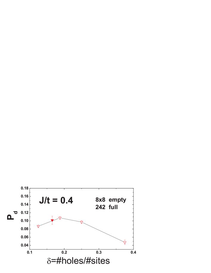
Figure 1: Superconducting order parameter $P_{d}$ for the 2D $t-J$ model as a function of doping, at $J/t=0.4$, calculated using variance extrapolation, using the projected BCS wave function defined in the text as an initial guess. Data taken from Ref. [6]

One of the most non trivial questions which arise in a strongly correlated regime is whether the ground state of a system containing only repulsive interaction can be superconductor. Surely such a state will not be found by any mean-field theory, which needs an explicit or effective attractive interaction in order to display a pairing strength among the electrons. Instead this question can be addressed at least at the variational level, dealing directly with strongly correlated variational wave functions which may exhibit a superconducting behavior and be close to the true GS of the system. Of course a clear indicator of the presence of superconductivity is the SC order parameter $P_{d}$, but since its value is of the same order as the quasiparticle weight, it can be too small to be detected with a reasonable numerical precision. Therefore, with the aim of finding a good probe for superconductivity, E. Plekhanov et al. [7] defined a new suitable quantity $Z_{c}$, which measure the pairing strength between two electrons added to the GS wave function,

$$Z_{c}=|F(\mathrm{shortest~{}distance})|/\sqrt{\sum_{all~{}distances}F^{2}(R)},$$ (4)

where $F(R)$ is related to the real space anomalous part of the equal time Green function at zero temperature:

$$F(R)=\langle N-2|c_{i,\uparrow}c_{i+R,\downarrow}+c_{i+R,\uparrow}c_{i,\downarrow}|N\rangle.$$ (5)

For instance $Z_{c}=0$ for Fermi liquids, instead $Z_{c}\neq 0$ for superconductors but also for non BCS systems which involve any kind of pairing. The authors in Ref. [7] applied this scheme to the 2D Hubbard model

$$H=-t\sum_{<i,j>,\sigma}\tilde{c}^{\dagger}_{i,\sigma}\tilde{c}_{j,\sigma}+h.c.+U\sum_{i}n_{i,\uparrow}n_{i,\downarrow}-\mu N,$$ (6)

where $\mu$ is the chemical potential and $N$ is the total number of particles. Carrying out a projection Monte Carlo technique based on auxiliary fields, they found that the GS of the undoped 2D Hubbard model at half filling has a non vanishing pairing strength, although the system is an insulator with antiferromagnetic long range order. This means that it is not a band insulator, for which $Z_{c}$ should be zero, but an RVB Mott insulator with a strong d–wave pairing character: indeed the RVB variational wave function is very close to the projected GS, giving the same pairing strength and a good variational energy. Moreover, the pairing strength decreases with increasing doping, but it is still positive for the lightly doped Hubbard model, suggesting that the system is ready to become superconductor, once the pairs can condense and phase coherence can take place in the GS.

The accuracy of the RVB ansatz close to the Mott insulator transition (MIT) has been pointed out also by Capello et al. [8], who undertake a variational Monte Carlo study of the phases of the $t-t^{\prime}$ 1D Hubbard model with nearest and next nearest neighbor hopping terms. The phase diagram of this model is known from bosonization and density-matrix renormalization group calculations, therefore it represents a good test case for the RVB variational wave function. When $t^{\prime}/t\lesssim 0.5$, the presence of a long range Jastrow factor acting on a BCS state is a crucial ingredient to recover the insulator with one electron per unit cell and without a broken translational symmetry, i.e. an highly non trivial charge gapped state. On the other hand, once $t^{\prime}/t\gtrsim 0.5$ and $U/t$ is small, the same wave function after optimization is able to describe the metallic state with strong superconducting fluctuations, namely a state with a finite spin gap. The distinction between the metallic and the insulating state can be made both by using the Berry phase[9] and by analyzing the behavior of the spin and charge structure factor as $q\rightarrow 0$; in all cases, the RVB state with an appropriate Jastrow factor reproduces very well the known phases.

Not only the conducting properties of a strongly correlated model can be reproduced by the RVB ansatz, but also the magnetic behavior. For instance, in the case of the $t-t^{\prime}$ 1D Hubbard model, the variational wave function drives the transition from the metallic to a dimerized insulator once $U/t$ increases. For the 2D spin 1/2 AFM Heisenberg model on a triangular lattice

$$H=J~{}\sum_{<i,j>}\mathbf{S}_{i}\cdot\mathbf{S}_{j}+J^{\prime}~{}\sum_{<<i,j>>}\mathbf{S}_{i}\cdot\mathbf{S}_{j},$$ (7)

with $J$ being the intra chain coupling and $J^{\prime}$ the inter chain one, the RVB wave function displays a stable spin liquid behavior, due to the strong frustration of the system in the regime with $J^{\prime}/J=0.33$. Moreover for $J=0.374meV$, the model is able to represent a real system, the $Cs_{2}CuCl_{4}$ compound studied by Coldea et al.[10, 11] who performed neutron scattering experiments in order to determine the low lying magnetic excitations. It turns out that the experimental data show an unconventional behavior of the magnetic structure of the compound, with spin-1/2 fractionalized excitations and incommensurability. The numerical study carried out in Ref. [12] highlights that the incommensurability comes from the frustration of the system and it is well described by the RVB ansatz. The most impressive correspondence between the experimental data and the numerical simulations is in the spin-1 excitation spectrum (see Fig.2), obtained by GFMC calculations with an RVB state used as a guiding function. As also shown in the same Fig. 2, it is evident that size effects are small and the comprairson between the numerical simulation and the experiment is particularly meaningful in this case. This is possible within a Quantum Monte Carlo (QMC) scheme that allows to work with large enough systems sizes.

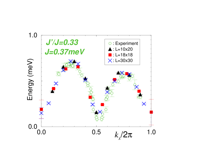
Figure 2: Comparison of the lowest triplet excitations, evaluated by neutron scattering experiments on $Cs_{2}CuCl_{4}$ compound[11], with the QMC results, obtained using the lattice fixed node approximation and the projected BCS state to approximate the signs of the ground state wave function[12]. There is no fitting parameter in the above comparison.

3 Realistic systems

As we have seen in the preceding section, the RVB wave function can represent very well the GS of some strongly correlated systems, which are described by a suitable lattice model, as in the case of $Cs_{2}CuCl_{4}$. Furthermore, following the seminal idea of Pauling, the applicability of the RVB ansatz is not limited to the strongly correlated regime close to the Mott transition or to spin frustrated models, but can be extended to describe the electronic structure and the properties of realistic systems. Indeed the quantum chemistry community has quite widely used the concept of pairing in order to develop a variational wave function able to capture the most significant part of the electronic correlation. Although only in 1987 Anderson discovered the link between the explicit resonating valence bond representation and the projected-BCS wave function, already in the 50’ s Hurley et al. [13] introduced the product of pairing functions as ansatz in quantum chemistry. Their wave function was called antisymmetrized geminal power (AGP) that has been shown to be the particle conserving version of the BCS ansatz [14]. It includes the single determinantal wave function, i.e. the uncorrelated state, as a special case and introduces correlation effects in a straightforward way, through the expansion of the pairing function (in this context called geminal): therefore it was studied as a possible alternative to the other multideterminantal approaches, but his success to describe correlation was very much limited, because - we believe - the Jastrow term was not included.

For an unpolarized system containing $N$ electrons (the first $N/2$ coordinates are referred to the up spin electrons) the AGP wave function is a $\frac{N}{2}\times\frac{N}{2}$ pairing matrix determinant, which reads:

$$\Psi_{AGP}(\textbf{r}_{1},...,\textbf{r}_{N})=\det\left(\Phi_{AGP}(\textbf{r}_{i},\textbf{r}_{j+N/2})\right)~{}~{}{\rm for}~{}1\leq i,j\leq N/2,$$ (8)

and the geminal function is expanded over an atomic basis:

$$\Phi_{AGP}(\textbf{r}^{\uparrow},\textbf{r}^{\downarrow})=\sum_{l,m,a,b}{\lambda^{l,m}_{a,b}\phi_{a,l}(\textbf{r}^{\uparrow})\phi_{b,m}(\textbf{r}^{\downarrow})},$$ (9)

where indices $l,m$ span different orbitals centered on atoms $a,b$, and $i$,$j$ are coordinates of spin up and down electrons respectively. It is possible to generalize the AGP many body wave function in order to deal also with a polarized system. The geminal function may be viewed as an extension of the simple HF wave function and in fact it coincides with HF only when the number $M$ of non zero eigenvalues of the $\lambda$ matrix is equal to $N/2$. It should be noticed that Eq. 9 is exactly the pairing function in Eq. 2, apart from the inhomogeneity of the former which reflects the absence of the translational invariance of a generic molecular compound. One of the main advantages of dealing with an AGP wave function is its computational cost. Indeed one can prove that expanding the geminal by adding more terms in the sum of Eq. 9 is equivalent to introduce more Slater determinants in the many body wave function, i.e. to have a multireference total wave function, similar to those obtained in configuration interaction (CI) or coupled cluster (CC) theories. But the computational cost of the AGP ansatz still remains the same, since one needs to compute always just a single determinant. This property is expected to be important for large scale simulations, since the number of determinants necessary for a satisfactory accuracy increases fast with the system size, limiting very much the applicability of CI and CC methods.

The simplest example which shows the essence of the AGP ansatz is the $H_{2}$ molecule. It is well known from textbooks that molecular orbital (MO) theory at the HF level fails in predicting the binding energy and the bond length of $H_{2}$, just because it overestimates the ionic terms contribution in the total wave function if the antibonding molecular orbitals are not included. In spite of this, the correct geminal expansion reads

$$\Phi_{AGP}(\textbf{r},\textbf{r}^{\prime})=\lambda\phi^{A}_{1s}(\textbf{r})\phi^{A}_{1s}(\textbf{r}^{\prime})+\phi^{A}_{1s}(\textbf{r})\phi^{B}_{1s}(\textbf{r}^{\prime})+A\leftrightarrow B,$$ (10)

where $\lambda$ can be tuned to regulate the weight of the different resonating contributions and fulfill the size consistency when the two nuclei are infinitely apart from each other ($\lambda\rightarrow 0$). Notice also that the chemical bond is represented in the geminal by a non vanishing value of $\lambda$ between the orbitals centered on the two different sites between which the bond is formed.

Let us consider now a gas of hydrogen dimers: in this case the geminal will contain not only the terms in Eq. 10, valid for just two sites, but also the contributions from all the nuclei in the system. It is clear that the AGP wave function will allow strong charge fluctuations around each $H$ pair, and therefore molecular sites with zero and four electrons are permitted, leading to poor variational energies. For this reason, the AGP alone is not sufficient, and it is necessary to introduce a Gutzwiller-Jastrow factor in order to dump the expensive charge fluctuations. Moreover only the AGP-Jastrow (AGP-J) wave function is the real counterpart of the RVB ansatz of strongly correlated lattice models, since the projection is essential to get the correct distribution of the pairing in the compound. The AGP-J wave function has shown to be effective both in atomic [15] and in molecular systems[16]. Both the geminal and the Jastrow play a crucial role in determining the remarkable accuracy of the many body state: the former permits the correct treatment of the nondynamic correlation effects, the latter allows the local conservation of charge in a complex molecular system and also to fulfill the cusp conditions which make the geminal expansion rapidly converging to the lowest possible variational energies.

The study of the AGP-J variational ansatz with the inclusion of two and three body Jastrow factors is possible by means of QMC techniques, which can deal explicitly with correlated wave functions. The optimization procedure, necessary to reach the lowest variational energy within the given variational freedom, is feasible also in a stochastic Monte Carlo framework, after the recent developments in this field ([17, 18]).

Benzene is the largest compound we have studied so far; in order to represent its ${}^{1}A_{1g}$ GS we have used a very simple one particle basis set: for the AGP, a 2s1p double zeta (DZ) Slater set centered on the carbon atoms and a 1s single zeta (SZ) on the hydrogen. For the 3-body Jastrow, a 1s1p DZ Gaussian set centered only on the carbon sites has been chosen. We started from a non resonating 2-body Jastrow wave function, which dimerizes the ring and breaks the full rotational symmetry, leading to the Kekulé configuration. As we expected, the inclusion of the resonance between the two possible Kekulé states lowers the variational Monte Carlo (VMC) energy by more than 2 eV. The wave function is further improved by adding another type of resonance, that includes also the Dewar contributions connecting third nearest neighbor carbons. As reported in Tab. 1, the gain with respect to the simplest Kekulé wave function amounts to 4.2 eV, but the main improvement arises from the further inclusion of the three body Jastrow factor, which allows to recover the $89\%$ of the total atomization energy at the VMC level. The main effect of the three body term is to keep the total charge around the carbon sites to approximately six electrons, thus penalizing the double occupation of the $p_{z}$ orbitals.

Table 1: Binding energies in $eV$ obtained by variational ($\Delta_{VMC}$) and diffusion ($\Delta_{DMC}$) Monte Carlo calculations with different trial wave functions for benzene. In order to calculate the binding energies yielded by the two–body Jastrow, we used the atomic energies reported in Ref. [15]. The percentages ($\Delta_{VMC}(\%)$ and $\Delta_{DMC}(\%)$) of the total binding energies are also reported. Data are taken from Ref. [16].

	$\Delta_{VMC}$	$\Delta_{VMC}(\%)$	$\Delta_{DMC}$	$\Delta_{DMC}(\%)$
Kekulé + 2body	-30.57(5)	51.60(8)	-	-
resonating Kekulé + 2body	-32.78(5)	55.33(8)	-	-
resonating Dewar Kekulé + 2body	-34.75(5)	58.66(8)	-56.84(11)	95.95(18)
Kekulé + 3body	-49.20(4)	83.05(7)	-55.54(10)	93.75(17)
resonating Kekulé + 3body	-51.33(4)	86.65(7)	-57.25(9)	96.64(15)
resonating Dewar Kekulé + 3body	-52.53(4)	88.67(7)	-58.41(8)	98.60(13)
full resonating + 3body	-52.65(4)	88.869(7)	-58.30(8)	98.40(13)

A more clear behavior is found by carrying out diffusion Monte Carlo (DMC) simulations: the interplay between the resonance among different structures and the Gutzwiller-like correlation refines more and more the nodal surface topology, thus lowering the DMC energy by significant amounts. Therefore it is crucial to insert into the variational wave function all these ingredients in order to have an adequate description of the molecule. For instance, in Fig. 3 we report the density surface difference between the non-resonating 3-body Jastrow wave function, which breaks the $C_{6}$ rotational invariance, and the resonating Kekulé structure, which preserves the correct $A_{1g}$ symmetry: the change in the electronic structure is significant. The best result for the binding energy is obtained with the Kekulé Dewar resonating 3 body wave function, which recovers the $98,6\%$ of the total atomization energy with an absolute error of 0.84(8) eV. As Pauling [1] first pointed out, benzene is a genuine RVB system, indeed it is well described by the AGP-J wave function.

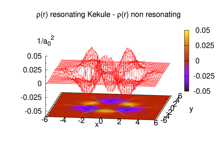
Figure 3: Electron density (atomic units) projected on the plane of $C_{6}H_{6}$. The surface plot shows the difference between the resonating valence bond wave function, with the correct $A_{1g}$ symmetry of the molecule, and a non-resonating one, which has the symmetry of the Hartree–Fock wave function.

4 Conclusions

In this paper we have described a very powerful variational ansatz that has been introduced to understand the properties of strongly correlated materials just after the discovery of HTc superconductivity. We have shown that the RVB wave function paradigm is not only useful for describing the GS and low lying excitations of lattice models, such as Heisenberg or $t-J$ model, but is also suited for approaching realistic systems, by considering explicitly the long range Coulomb repulsion and the full quantum mechanical interaction among electrons within the Born-Oppenheimer approximation. Moreover, by using the same type of wave function both for lattice model and realistic system, it is possible to have some insight in the electron correlation behind the latter and to check the reliability of the model in predicting the properties of a real compund. For instance the benzene molecule can be idealized by a six site ring Heisenberg model with one electron per site, in order to mimic the out of plane bonds of the real molecule, coming from the $p_{z}$ electrons and leading to an antiferromagnetic superexchange interaction between nearest neighbor carbon sites. We have studied in this case the spin–spin correlations

$$C(i)=\langle S^{z}_{0}S^{z}_{i}\rangle,$$ (11)

where the index $i$ labels consecutively the carbon sites starting from the reference $0$, and the dimer–dimer correlations

$$D(i) = D_{0}(i)/C(1)^{2}-1,$$

$$D_{0}(i) = \langle(S^{z}_{0}S^{z}_{1})(S^{z}_{i}S^{z}_{i+1})\rangle.$$ (12)

Both correlation functions have to decay in an infinite ring, when there is neither magnetic ( $C(i)\to 0$ ), nor dimer ($D(i)\to 0$) long range order as in the true spin liquid ground state of the 1D Heisenberg infinite ring.

Indeed, as shown in the inset of Fig.(4), the dimer–dimer correlations of benzene are remarkably well reproduced by the ones of the six site Heisenberg ring, whereas the spin–spin correlation of the molecule appears to decay faster than the corresponding one of the model. Though it is not possible to make conclusions on long range properties of a finite molecular system, our results suggest that the benzene molecule can be considered closer to a spin liquid, rather than to a dimerized state, because, as well known, the Heisenberg model ground state is a spin liquid and displays spontaneous dimerization only when a sizable next-nearest frustrating superexchange interaction is turned on.[19]

Figure 4: Spin–spin correlation function for benzene (full squares) and for the Heisenberg model (empty circles). In the inset, also the dimer–dimer correlation function is reported with the same notation. For the benzene molecule, these correlation are obtained by a coarse grain analysis in which the “site” is defined to be a cylinder of radius $1.3~{}a_{0}$ centered on the carbon nuclei, with a cut off core (i.e. we considered only the points with $|z|>0.8~{}a_{0}$). All the results are pure expectation values obtained from forward walking calculations.

As any meaningful variational ansatz, the RVB approach naturally brings a new way of understanding the many-body problem, as for instance the Hartree-Fock theory helped to interpret the periodic table of elements, or to establish on theoretical grounds the band theory of insulators. With the RVB paradigm, many unusual phenomena now appear to be possibly explained in a simple and consistent framework: the role of correlation in Mott insulators, or the explanation of HTc superconductivity, and finally the fractionalization of spin excitations, which was supposed to take place only in quasi-one dimensional systems, and instead it has been recently detected in higher dimensions.[10] All these phenomena cannot be understood not even qualitatively within a mean field Hartree–Fock theory, as the important ingredient missing in the latter approach is just the correlation, that can lead to essentialy new effects.

In our opinion the RVB wave function is a natural extension of the Hartree-Fock one, to which it reduces whenever the correlation term is switched off. In some sense the determinantal part is useful to represent the electronic density and all the one body properties of an electronic system. On the other hand the Jastrow term is necessary to take correctly into account the density–density correlation, $N(r)=<n_{0}n_{r}>$. The long range behavior of $N(r)$ discriminates a metal, displaying Friedel oscillations at $4k_{F}$ where $k_{F}$ is the Fermi momentum, from an insulator, which shows an exponentially localized correlation $N(r)\simeq\exp(-r/\xi)$, where $\xi$ is the corresponding characteristic length. The Jastrow correlation can become non trivial when the determinantal part acquires a non conventional meaning. For instance, the determinantal part in the RVB wave function could describe a superconductor or a metal, but the presence of the Jastrow factor is able to turn the system into an insulator, by correlating the electrons in a non trivial way. On the other hand, superconductivity can naturally become stable in a system with only repulsive interactions, despite the BCS theory would require an effective attraction mediated by the phonons.

For all the above reasons we believe that it is the right time to make an effort to study complex electronic systems by means of this new paradigm, especially for discovering new challenging effects in which the role of correlation is dominant.

References

- [1] L. Pauling, The nature of the chemical bond, Cornell University Press, Ithaca, New York, Third edition.
- [2] P. W. Anderson, Mater. Res. Bull. (8) (1973) 153.
- [3] P. W. Anderson, Science (235) (1987) 1196.
- [4] J. G. Bednorz, K. A. Muller, Z. Phys. (B64) (1986) 189.
- [5] P. W. Anderson, P. A. Lee, M. Randeria, T. M. Rice, N. Trivedi, F. C. Zhang, cond-mat/0311467.
- [6] S. Sorella, G. B. Martins, F. Becca, C. Gazza, L. Capriotti, A. Parola, E. Dagotto, Phys. Rev. Lett. (88) (2002) 117002.
- [7] E. Plekhanov, F. Becca, S. Sorella, cond-mat/0404206.
- [8] M. Capello, F. Becca, M. Fabrizio, S. Sorella, E. Tosatti, cond-mat/0403430.
- [9] R. Resta, S. Sorella, Phys. Rev. Lett. (74) (1995) 4738.
- [10] R. Coldea, D. A. Tennant, A. M. Tsvelik, Z. Tylczynski, Phys. Rev. Lett (86) (2001) 1335.
- [11] R. Coldea, D. A. Tennant, Z. Tylczynski, Phys. Rev. B (68) (2001) 134424.
- [12] S. Yunoki, S. Sorella, Phys. Rev. Lett (92) (2004) 157003.
- [13] A. C. Hurley, J. E. Lennard-Jones, J. A. Pople, Proc. R. Soc. London (Ser. A 220) (1953) 446.
- [14] J. R. Schrieffer, The Theory of Superconductivity, Addison–Wesley, 5th printing, 1994.
- [15] M. Casula, S. Sorella, J. Chem. Phys. (119) (2003) 6500.
- [16] M. Casula, C. Attaccalite, S. Sorella, cond-mat/0409644.
- [17] S. Sorella, Phys. Rev. B (64) (2001) 024512.
- [18] F. Schaultz, C. Filippi, J. Chem. Phys. (120) (2004) 10931.
- [19] S. White, I. Affleck, Phys. Rev. B (54) (1996) 9862.