Distribution Functions, Loop Formation Probabilities and Force-Extension Relations in a Model for Short Double-Stranded DNA Molecules

Abstract

We obtain, using transfer matrix methods, the distribution function $P(R)$ of the end-to-end distance, the loop formation probability and force-extension relations in a model for short double-stranded DNA molecules. Accounting for the appearance of “bubbles”, localized regions of enhanced flexibility associated with the opening of a few base pairs of double-stranded DNA in thermal equilibrium, leads to dramatic changes in $P(R)$ and unusual force-extension curves. An analytic formula for the loop formation probability in the presence of bubbles is proposed. For short heterogeneous chains, we demonstrate a strong dependence of loop formation probabilities on sequence, as seen in recent experiments.

The physics of bending and loop formation in DNA is key to a variety of regulatory processes within the cell. Loop formation in DNA is believed to be central to enhancer action, while the compactness of DNA packaging within the nucleosome necessitates the bending of DNA over length scales of a few tens of base pairs kadonaga-98 ; alberts . In a broader context, the modelling of bending and looping in biopolymers at length scales over which intrinsic stiffness plays a dominant role is a problem of general relevance.

Worm-like chain (WLC) models of DNA elasticity incorporate semi-flexibility, describing the chain in terms of a persistence length $l_{p}$, the length-scale at which tangent vectors to the polymer are decorrelated doi-ed . On scales smaller than $l_{p}$, bending energy dominates and the chain is relatively stiff. It has conventionally been assumed that the relatively large energy required to bend short double stranded (ds) DNA of length $L\sim 100$  base-pairs (bp) into loops necessitates the intervention of DNA-binding proteins. Recent DNA cyclization experiments of Cloutier and Widom (CW) which study relatively small, isolated  dsDNA sequences question this assumption cw . In the CW experiments, DNA molecules that are 94 bp in length, comparable to sharply looped DNAs in vivo, spontaneously cyclize with a large probability. Theories of DNA elasticity based on the homogeneous WLC model predict cyclization probabilities three to four orders of magnitude smaller than those obtained experimentally shimada-yamakawa , indicating, in the words of Cloutier and Widom, “a need for new theories of DNA bending” cw .

The problem posed by these experiments has stimulated much recent work on modelling loop formation in short DNA moleculesyan-marko ; wiggins-nelson-kink . An attractive explanation for this discrepancy is the existence of “bubbles”, localized regions of large flexibility induced by the opening of a few base pairs of dsDNA in thermal equilibrium yan-marko . (Alternatively, it has been argued that non-linear elastic effects relevant at high curvature might induce a kinking transitionwiggins-nelson-kink .) Bubbles (or kinks) are argued to greatly increase the flexibility of the WLC in their vicinity, thereby enhancing the cyclization probabilityyan-marko ; wiggins-nelson-kink . Recent transfer-matrix based calculations implement this idea, but restrict themselves to the computation of the cyclization probabilityyan-marko .

In this Letter we report the first calculation of the distribution function of the end-to-end distance $P(R)$ in a model for short dsDNA fragments with equilibrium bubbles. We propose an analytic formula describing the loop formation probability density $P(0)$ in such fragments and compare this formula with results from numerical calculations. Varying the chemical potential for bubbles leads to behaviour which interpolates between fully flexible, semiflexible and rigid rod limits, resulting in a variety of non-trivial force-extension curves. Simple extensions of our model which simulate DNA heterogeneity indicate that such heterogeneities can be important determinants of the cyclization probability in small chains.

We use the well-known connection of the WLC model, with hamiltonian $H_{WLC}=\kappa/2\int_{0}^{L}ds\left(\partial{\bf t}(s)/\partial s\right)^{2}$ constrained by $|{\bf t}^{2}(s)|=1$, to the Heisenberg spin model  fisher ; bensimon . Here ${\bf t}(s)\equiv\partial{\bf r}(s)/\partial s$ is the unit tangent vector and $\kappa$ is the bending stiffness. The persistence length is $l_{p}=\beta\kappa$ with $\beta=1/k_{B}T$. Mapping the continuum model to the discrete one requires that a minimum coarse-graining length scale be specified. We fix this to be $b=1$ nm (3 bp’s). (This also represents the scale at which the smallest bubbles appear.) Thus, a 150 bp chain is represented by an L=50 site spin model. In what follows, both $L$ and $l_{p}$ are dimensionless numbers representing the physical chain length and persistence length in units of this basic scale. The bending stiffness and the coupling constant in the spin model are related through $J=\kappa/b$. In the WLC model, the distribution function of the end-to-end vector $P({\bf R})$ characterizes the conformations of the polymer; it depends only on the ratio $L/l_{p}$. Rotational invariance imposes $P({\bf R})=P(|{\bf R}|)=P(R)$.

The energetics of ds DNA in the presence of bubbles in equilibrium is modelled via the following hamiltonianyan-marko

$$H=\sum_{i=1}^{N-1}\left[\tau_{i}J_{s}(1-\hat{\bf t}_{i}\cdot\hat{\bf t}_{i+1})+(1-\tau_{i})J_{d}(1-\hat{\bf t}_{i}\cdot\hat{\bf t}_{i+1})\right]-{\mathrm{\mu}}\sum_{i=1}^{N-1}(1-\tau_{\mathrm{i}}).$$ (1)

Here $\tau_{i}$ is a local variable which specifies whether a given bond forms part of a bubble or not: $\tau_{i}=1$ if the site $i$ is a part of the bubble, otherwise $\tau_{i}=0$. A chemical potential $\mu$ controls the energetics of the $\tau_{i}$ variable and hence the number of bubbleslavery . The bending stiffness of double-stranded and bubble regions map to coupling constants $J_{d}$ and $J_{s}$ respectively.

The distribution function $P({\bf R})$ of the end-to-end vector ${\bf R}=\sum_{i=1}^{N}\hat{{\bf t}}_{i}$ is

$$P({\bf R})=\mathcal{N}\int d{\bf t}_{1}\ldots\int d{\bf t}_{N}\sum_{\tau_{1}=0}^{1}...\sum_{\tau_{N-1}=0}^{1}e^{-\beta H}\delta(\sum_{i}^{N-1}{\hat{\bf t}}_{i}-\bf{R}),$$ (2)

where ${\mathcal{N}}$ fixes $\int d{\bf R}P(R)=1$. With one end of the polymer at ${\bf R}=0$, the probability $p(z)$ for the other to be in a given $z$-plane is related to $P({\bf R})$ through $p(z)=\int d{\bf R}P(R)\delta(R_{3}-z)$, where ${\bf R}=R_{1}\hat{e}_{x}+R_{2}\hat{e}_{y}+R_{3}\hat{e}_{z}$. Defining a generating function $\tilde{p}(f)$ sam through $\tilde{p}(f)=\int_{-L}^{L}dz~{}\exp(fz)p(z)$, yields, upon substituting definitions of $p(z)$ and $P(R)$, the relation $\tilde{p}(f)=Z(f)/Z(f=0)$, where $Z(f)=\int d{\bf t}_{1}\ldots\int d{\bf t}_{N}\sum_{\tau_{1}=0}^{1}...\sum_{\tau_{N-1}=0}^{1}\exp{(-\beta H+f\sum_{i=1}^{N}\hat{t}_{i}^{z}))}$. After performing the $\tau_{i}$ summation, $Z(f)$ can be computed using transfer matrices blume . Once $Z(f)$ is known, $\tilde{p}(f)$ and $p(z)$ can be computed. $P(R)$ is then finally obtained, exploiting the tomographic methods outlined in Ref. sam and symmetry arguments, from $P(R)=(-1/2\pi z)dp(z)/dz|_{z=R}$. We can either allow the tangent vectors at the two ends to fluctuate independently, corresponding to free boundary conditions on the tangent vectors, or require that they be equal, a boundary condition believed to be appropriate to the CW experiments.

We benchmark our methods by computing $P(R)$ for a homogeneous semiflexible polymer in the absence of bubbles, (i.e. $\mu=\infty$), at various $L/l_{p}$ values. Our approach yields results which are fully consistent with previous work, reproducing known answers from simulations and analytic work marko-siggia ; frey . In addition, for $L/l_{p}=3.85$, we recover the double hump feature in the distribution function reported recently abhishek ; sam . We have also computed the loop formation probability density $P(0)$ (defined as $P(R=0)$) for the entire range of $L/l_{p}$ values, obtaining results which agree well with the Shimada-Yamakawa formulashimada-yamakawa .

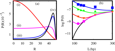
Figure 1: (a) $P(R)$ calculated for a $150$ bp DNA fragment with $\beta J_{d}=50$ and $\beta J_{s}=1$ for (i)$\beta\mu=6$, (ii) $\beta\mu=7$ and (iii) $\beta\mu=9$. The curve (iv) is $P(R)$ from the WLC calculations($\beta\mu=\infty$). (b) $P(0)$ from the transfer matrix calculation (points) compared to the predictions of the aproximate formula of Eq. 4 (lines). The curves from top to bottom are for $\beta\mu=10,12,15,18$ and $\infty$.

To incorporate bubble formation, we fix $\beta J_{d}=50$ for the double stranded region and $\beta J_{s}=1$ for the bubble region, consistent with measures of the persistence length notewell . Our results for $L=50$ are plotted in Fig. 1(a) for $\beta\mu=6,7$ and $9$. (The free energy cost in units of temperature $\beta\mu$ to form a $3$bp bubble can be estimated to lie between $6$ and $15$ depending on the sequence yan-marko ). For $\beta\mu=6$ the distribution function peaks at $R=0$. Remarkably, for $\beta\mu=9$, the distribution function alters completely, with the peak shifting to near $R=L$. For intermediate values of $\mu$, the peak of $P(R)$ interpolates between $R=0$ and $R\simeq L$. For $L/l_{p}=1$, $P(R)$ exhibits a double hump feature when $\beta\mu=6.9$, as described earlier for semiflexible chains in the regime in which $L/l_{p}\sim 3.85$.

The loop formation probability density $P(0)$ is experimentally accessible. Fig. 1(b) shows $P(0)$ (symbols) at different values of $\mu$, as $L$ is varied. The boundary condition imposed allows the tangent vectors at the chain ends to fluctuate independently. The lines through the data points are predictions of the analytic theory described below. At large $\mu$, the results asymptote to those obtained for $\mu\rightarrow\infty$. As $\mu$ is decreased from infinity, bubbles are favoured and $P(0)$ increases sharply at small $L$.

We have specialized our calculations to allow for the insertion of a single bubble at arbitrary points along the chain. This allows us to check for the optimal bubble location. We compute $P(R)$ for the case in which a single bubble is placed at the centre ($L/2)$ as well as at positions which deviate from the central position by one and two sites on both sides, as shown in Fig. 2. At the parameter values $\beta J_{d}=L=50$, the distribution function is peaked sharply near $L$. Allowing for a single bubble at the centre transforms $P(R)$ completely, shifting the peak to $R=0$. The peak of the distribution function moves away from $R=0$, as the bubble position moves off-centre, with $P(R)$ peaking near $R=L$ as the bubble position shifts to the chain end. We plot $P(0)$ as a function of the bubble position in the inset to Fig 2. As the bubble position moves 3 units away from the center, $P(0)$ drops by one order of magnitude. This peak at $L/2$ becomes sharper for small $L$, implying that the principal contribution to the loop forming probability density for short chains comes from bubbles positioned at the chain center.

This observation justifies a simple analytic approach to $P(R)$ and the loop formation probability density: The distribution function $P(R)$ for short DNA molecules ($L\ll l_{p}$, so they may be assumed to be rigid to a first approximation) with one bubble in the middle can be represented in terms of two infinitely rigid rods of length $L/2$ connected with a flexible hinge. In the limit where the bending energy cost at the hinge is zero, the probability distribution function is that of a random walk with two steps of equal size $L/2$. This yields $P(R)=1/(2\pi L^{2}R)$, a behavior similar to that obtained from the transfer matrix calculation; see the top curve of Fig. 2 (main panel).

Analytic results beyond the assumption of rigid rod behaviour can be derived for the loop formation probability density at large $\mu$, at which the effects of a single bubble dominate. We have found that the distribution function of the end-to-end vector $P({\bf R},L,l_{p})$ for a semiflexible chain of length $L$ with a persistence length $l_{p}$ in a regime relevant to the DNA molecules in the CW experiment, is dominated by the weighted sum of two terms. The first term, $P_{0}(l_{p},L)$, is the contribution in the absence of bubbles, while the second, $P_{1}(l_{p},L)$, reflects the contribution from a single bubble placed at the centre of the chain. Thus, $P({\bf R},L,l_{p})$ in the limit ${\bf R}\rightarrow 0$, the loop formation probability density, is then

$$P(0)\simeq\frac{1}{1+2l_{p}e^{-\beta\mu}}\left[P_{0}(l_{p},L)+2l_{p}e^{-\beta\mu}P_{1}(l_{p},L)\right].$$ (3)

(The factors of $2l_{p}e^{-\beta\mu}$ are fixed by the normalization appropriate to the calculation of the loop formation probability density from the spin model.) The Shimada-Yamakawa theory of the cyclization of semiflexible polymers provides quantitative estimates of $P_{0}(l_{p},L)$shimada-yamakawa in the limit relevant to the Cloutier-Widom experiments.

The term $P_{1}(l_{p},L)$ represents the loop forming probability density of a chain of length $L$ with a flexible hinge in the center. We exploit an accurate variational expression for the end-to-end distribution function of a semiflexible chain of length $L$ thirumalai-ha : $P({\bf R},L)=\frac{C(g)}{L^{3}}\left[\frac{1}{1-(R/L)^{2}}\right]^{9/2}\exp\left[\frac{g}{1-(R/L)^{2}}\right]$ with $g=9L/8l_{p}$, and obtain $P(0)$ from an integral over the product of $P({\bf R},L)$’s of the form $\int d{\bf R}P({\bf R},L/2)P(-{\bf R},L/2)$. This leads to $P_{1}(l_{p},L)=\left(\frac{32\pi C^{2}(g/2)}{L^{3}}\right)\int_{0}^{1}dxe^{f(x)}$, where $x=2R/L$ and $f(x)=2\ln x-9\ln(1-x^{2})-g/(1-x^{2})$, and $C(g/2)$ is a normalization factor thirumalai-ha . The integral is first approximated by saddle point techniques. We then multiply the resulting analytic expression by a further constant factor of 2.273, to match with results obtained through numerical integration. This procedure yields near perfect agreement with numerics in the range $0<L/l_{p}<3$; a range over which the integral varies across 12 orders of magnitude. Further specializing the resulting expression to the $L/l_{p}$ regime explored in the CW experiments yields a single formula for $P(0)$, involving $\beta\mu$ and $l_{p}$:

$$P(0) = \frac{1}{1+2l_{p}e^{-\beta\mu}}\left[112.04\frac{l_{p}^{2}}{L^{5}}e^{-14.055\frac{l_{p}}{L}+0.246\frac{L}{l_{p}}}\right.$$ (4)

$$+ \frac{18.31}{\pi^{\frac{3}{2}}l_{p}^{3}}~{}(2l_{p}e^{-\mu})\left.\frac{y^{2}{(1-y^{2})}^{\frac{-15}{2}}(1+\frac{16l_{p}}{3L}+\frac{320l_{p}^{2}}{27L^{2}})^{-2}e^{\frac{-9L}{8l_{p}}\left(\frac{y^{2}}{1-y^{2}}\right)}}{\left(36y^{4}-36y^{2}+\frac{27}{4}y^{2}\frac{L}{l_{p}}+\frac{9L}{4l_{p}}\right)^{\frac{1}{2}}}\right],$$

where $y^{2}=1.037-0.1667L/l_{p}$. This formula is compared to the results of the transfer matrix calculations in Fig. 1. The agreement is satisfactory, particularly at large $\mu$, where the “single bubble” approximation is expected to be accurate.

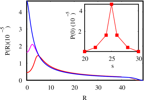
Figure 2: $P({\bf R})$ for homogeneous dsDNA of length $L=50$ computed with a single bubble placed at L/2 (top curve), $L/2\pm 1$ (middle curve) and $L/2\pm 3$ (bottom curve). The inset shows $P(0)$ as a function of bubble position, illustrating how this quantity peaks sharply when the bubble is placed at the centre.

Variations in $P(R)$ as a consequence of bubble formation should be reflected in experimentally measurable force extension (FE) relations. Experiments typically measure the average force required to maintain the two ends of the polymer at a fixed separation $R$. This average force is $\langle f\rangle=-\partial\log{(P(R))}/\partial R$. Since our calculations access $P(R)$ directly, we can calculate this average force as a function of extension in all the cases discussed earlier. We find that the FE curves are strongly ensemble dependent for small chains – FE relations in the fixed force ensemble are always monotonicwiggins-nelson-kink , while non-monotonic relations can be obtained in the fixed extension ensemble. Such non-monotonicity disappears in the $L\rightarrow\infty$ limit, where FE curves calculated in both ensembles coincide, as expected. Fig. 3 shows plots for homogeneous chains setting $\beta J=50$ and $\beta\mu=6$ and $9$, of $\langle f\rangle$ vs. R, in the constant extension ensemble (plots (b) and (a), respectively), as well as in the constant force ensemble, in which $\langle R\rangle$ vs. f is calculated (see plots (c) and (d)), illustrating these conclusions.

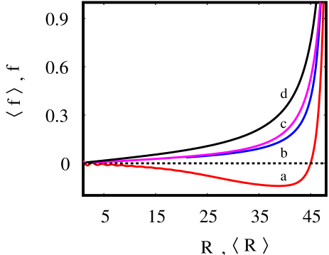
Figure 3: Force extension relation for homogeneous dsDNA of length $L=50$ at parameter values $\beta J=50$ with $\beta\mu=6$ and $\beta\mu=9$. The curves (a) and (b) are computed in the fixed-extension ensemble whereas the curves (c) and (d) are computed in the fixed force ensemble.

We have also investigated the effects of sequence heterogeneity on the loop formation probability density and $P(R)$. The energy to break paired bases is strongly sequence dependent, and alters the local value of $J$. (It is known that A-T bonds are more easily broken than G-C bonds alberts ; libchaber-bubble .) Intuitively, regions of reduced bending rigidity should play a role similar to that played by bubbles, reducing the energy required to bend the chain at specific locations. We have experimented with 50:50 mixtures of bonds with strength $\beta J=40$ (weak) and $\beta J=60$ (strong) in a system of size $L=100$ and arranged in the following way: (a) two equal stretches of strong bonds at each end, separated by 50 weak bonds in the central region (b) two equal stretches of weak bonds at each end, separated by 50 strong bonds in the central region and (c) a typical random sequence formed by laying weak and strong bonds down at random, subject to the constraint that they are equal in number. We have checked that in the limit of large chains, the results for a typical random sequence of weak and strong bonds are close to those obtained from the homogeneous case with $\beta J=50$.

Our results are the following: as is intuitively clear, the case in which the stretch of weak bonds is placed in the centre, case (a), yields the largest values for $P(0)$ while the case in which strong bonds populate the centre, case(b), yields the smallest. The random chain result, case (c), is close to the result for the homogeneous case. The variation in $P(0)$ spans a full order of magnitude or more for short chains at these parameter values, indicating the importance of sequence heterogeneity for loop formation.

In conclusion, we have computed a wide range of physical properties of a simple model for short dsDNA molecules which incorporates the presence of bubbles in equilibrium. We point out that several physical properties of short dsDNA molecules, as reflected in $P(R)$, are strongly affected by bubble formation. Our model is easily extended to account for sequence heterogeneity. The unusual force-extension relations in diverse ensembles exhibited here may have implications for loop formation in vivo.

We thank M. Rao and R. Siddharthan for discussions and J. Widom for sending us a copy of Ref.cw . PR acknowledges discussions with J. Marko and S. Sankararaman. This work was partially supported by the CSIR (India).

References

- (1) E. M. Blackwood and J. T. Kadonaga, Science, 281 60 (1998)
- (2) B. Alberts et. al., Molecular Biology of the Cell 4th ed, (Garland Science, 2002)
- (3) M. Doi and S.F Edwards, The Theory of Polymer Dynamics (Claredon Press, Oxford, 1986)
- (4) T. E. Cloutier and J. Widom Mol. Cell,14 355 (2004)
- (5) J. Shimada and H. Yamakawa, Macromolecules, 17, 689, (1984)
- (6) J. Yan and J. F. Marko, Phys. Rev. Lett., 93, 108108 (2004)
- (7) P. A. Wiggins, R. Phillips and P. C. Nelson, http://arxiv.org/abs/cond-mat/0409003
- (8) Regions of large curvature might favour bubble formation, a non-linear coupling which we ignore for simplicity; see J. Ramstein and R. Lavery, Proc. Natl. Acad. Sci. USA, 85, 7231, (1988).
- (9) M. E. Fisher, Am. J. Phys. 32 343 (1964)
- (10) D. Bensimon, D. Dohmi and M. Mézard, Europhys. Lett., 42(1), 97-102 (1998)
- (11) J. Samuel and S. Sinha, Phys. Rev. E 66, 050801(R) (2002)
- (12) M. Blume, P. Heller and N. A. Lurie, Phys. Rev. B 11 4483 (1975)
- (13) J. F. Marko and E. D. Siggia, Macromolecules, 28, 8759 (1995)
- (14) J. Wilhelm and E. Frey, Phys. Rev. Lett. 77, 2581 (1996).
- (15) A. Dhar and D. Chaudhuri, Phys. Rev. Lett. 89, 065502 (2002).
- (16) The measured of dsDNA is approximately while that of single stranded DNA is roughly . See e.g. S. B. Smith, Y. Cui, and C. Bustamante, Science, 271, 795 (1996).
- (17) D. Thirumalai and B.-Y. Ha, in Theoretical and Mathematical Models in Polymer Research, A. Grosberg, ed. (Academic Press, San Diego, CA, 1998).
- (18) G. Altan-Bonnet, A. Libchaber and O. Krichevsky, Phys. Rev. Lett. 90, 138101 (2003)