Capillary waves in a colloid–polymer interface

Abstract

The structure and the statistical fluctuations of interfaces between coexisting phases in the Asakura–Oosawa (AO) model for a colloid–polymer mixture are analyzed by extensive Monte Carlo simulations. We make use of a recently developed grand canonical cluster move with an additional constraint stabilizing the existence of two interfaces in the (rectangular) box that is simulated. Choosing very large systems, of size $L\times L\times D$ with $L=60$ and $D=120$, measured in units of the colloid radius, the spectrum of capillary wave–type interfacial excitations is analyzed in detail. The local position of the interface is defined in terms of a (local) Gibbs surface concept. For small wavevectors capillary wave theory is verified quantitatively, while for larger wavevectors pronounced deviations show up. For wavevectors that correspond to the typical distance between colloids in the colloid–rich phase, the interfacial fluctuations exhibit the same structure as observed in the bulk structure factor. When one analyzes the data in terms of the concept of a wavevector–dependent interfacial tension, a monotonous decrease of this quantity with increasing wavevector is found. Limitations of our analysis are critically discussed.

I Introduction

By adding non–adsorbing polymers to a colloidal suspension, phase separation may be induced. This leads to the formation of two coexisting phases, one with high colloid density and one with low colloid density, separated by an interface. The interface is not flat, but subject to thermally driven density fluctuations known as capillary waves. Capillary waves were first predicted by Smoluchowski von Smoluchowski (1908), and have since then been studied using light and X-ray diffraction Doerr et al. (1999); Fradin et al. (2000); Mora et al. (2003); Li et al. (2004), theoretical methods Huse et al. (1985); van Leeuwen and Sengers (1989); Sengers and van Leeuwen (1989); Napiórkowski and Dietrich (1993); Dietrich and Napiórkowski (1991); Mecke and Dietrich (1999), and computer simulations Schmid and Binder (1992); Werner et al. (1997); Stecki (1998); Binder and Müller (2000); Stecki (2001); Vink and Horbach (2004a). Recently, capillary waves were even visualized directly, close to single particle resolution, in a colloid–polymer mixture Aarts et al. (2004).

Figure 1: Schematic representation of an interface within the framework of capillary wave theory. The mesh shows the local interface position $z=h(x,y)$, which is assumed to be a smooth function of the lateral coordinates $x$ and $y$. The surface $h(x,y)$ then separates phase A (shaded lower region) from phase B (upper region).

Unlike critical fluctuations, capillary waves survive deep into the two–phase region of the phase diagram, and strongly influence all quantities that depend on transversal degrees of freedom. For example, the capillary contribution to the width of the interface diverges logarithmically with the lateral system size. As a consequence, the apparent width of the interface depends on the length scale on which it is studied. This effect is well described by capillary wave theory (CWT) Buff et al. (1965); Safran (1994), which consequently plays an important role in the modern treatment of interfaces. The key assumption is that a smooth local interface position can be defined, see Fig. 1. Clearly, away from any critical point, and for long wavelength capillary variations, this assumption is reasonable. However, at short wavelengths, say of the order of the particle diameter, the concept of a smooth local interface, and hence CWT, breaks down. Naturally, much effort has been devoted to extend CWT, in order to yield a valid description at short wavelengths Dietrich and Napiórkowski (1991); Napiórkowski and Dietrich (1993); Mecke and Dietrich (1999). The task is challenging, because a correct theory must interpolate between the continuum (long wavelength) CWT limit, to the microscopic (single–particle) limit at short wavelengths. In simulations and experiments, the situation is slightly less problematic. Here, model interfaces are readily prepared, and their properties can be probed relatively easily, on a wide range of different length scales.

In this work, Monte Carlo simulations are used to study capillary waves in a simple model of a colloid–polymer mixture. Our first aim is to test the long wavelength predictions of CWT. One of these predictions relates the capillary spectrum to the interfacial tension. The CWT estimate of the interfacial tension, is then compared to independent estimates, obtained by us in previous work. Next, we consider the short wavelength limit of the capillary spectrum. In this limit, we observe that the capillary spectrum approaches the static structure factor of the bulk liquid. Moreover, we find that the transition from the long wavelength CWT limit of the spectrum, to the short wavelength limit, is smooth. Our findings are then discussed in light of the Mecke–Dietrich theory Mecke and Dietrich (1999) for interfaces, and the recent experiment of Ref. Aarts et al., 2004.

The outline of this paper is as follows. We first discuss CWT. Next, we introduce the colloid–polymer model, and describe the simulation method. We then describe how the local interface position is extracted from raw simulation data. Finally, we present our results, and finish with a number of conclusions in the last section.

II Capillary wave theory

As stated before, the key assumption in CWT is the notion of a smooth interface, see Fig. 1. The local interface position $h(x,y)$ is written as a function of the lateral coordinates $x$ and $y$. By lateral, we mean those directions parallel to the plane containing the interface. The other important direction is the perpendicular direction. In this work, the lateral coordinates $(x,y)$ are restricted to the interval $[0,L]$, with $L$ the lateral dimension of the system. The perpendicular coordinate $z$ is restricted to $[0,D]$, with $D$ the perpendicular dimension of the system.

II.1 Capillary spectrum

The first step in deriving the capillary wave spectrum, is to write down the energy cost ${\cal H}_{\rm cw}$ of having a non–flat (or undulated) interface with respect to a perfectly flat one. Here, the subscript “cw” emphasizes that the energy cost is due to capillary waves. The energy can be expressed as the product of the interfacial tension $\gamma$ and the excess area $\Delta A$. The excess area is defined as the area of the undulated surface $h(x,y)$ minus the area of a perfectly flat interface, leading to Widom (1972); Weeks (1977); Rowlinson and Widom (1982); Jasnow (1984)

$$\frac{{\cal H}_{\rm cw}}{\gamma}=\Delta A=\int_{0}^{L}\int_{0}^{L}\sqrt{\nabla h\cdot\nabla h+1}\hskip 2.84526pt{\rm d}x\hskip 2.84526pt{\rm d}y-L^{2},$$ (1)

with gradient operator $\nabla=(\partial/\partial x,\partial/\partial y)$. As a first approximation, we assume $|\nabla h|\ll 1$, and thus

$${\cal H}_{\rm cw}\approx\frac{\gamma}{2}\int_{0}^{L}\int_{0}^{L}\nabla h\cdot\nabla h\hskip 2.84526pt{\rm d}x\hskip 2.84526pt{\rm d}y,$$ (2)

which defines the capillary wave Hamiltonian. Next, the local interface position is expressed as a two-dimensional Fourier series

$$h(x,y) = A_{00}$$

$$+ \sum_{n,m}A_{nm}\cos(\vec{x}\cdot\vec{q}_{nm})+B_{nm}\sin(\vec{x}\cdot\vec{q}_{nm}),$$

with $\vec{x}\equiv(x,y)$ and wavevector $\vec{q}_{nm}\equiv(2\pi n/L,2\pi m/L)$. In the above and following equations, the summation is over all pairs of integers $(n,m)$, with $n\geq 0$ and $m\geq 0$, excluding the pair $(0,0)$. The Fourier amplitudes are given by

$$A_{nm} = \frac{1}{L^{2}}\int_{0}^{L}\int_{0}^{L}h(x,y)\cos(\vec{x}\cdot\vec{q}_{nm})\hskip 2.84526pt{\rm d}x\hskip 2.84526pt{\rm d}y,$$ (4)

$$B_{nm} = \frac{1}{L^{2}}\int_{0}^{L}\int_{0}^{L}h(x,y)\sin(\vec{x}\cdot\vec{q}_{nm})\hskip 2.84526pt{\rm d}x\hskip 2.84526pt{\rm d}y.$$ (5)

The capillary wave Hamiltonian of Eq.(2) now takes the quadratic form

$${\cal H}_{\rm cw}=\frac{\gamma L^{2}}{4}\sum_{n,m}\left(A_{nm}^{2}+B_{nm}^{2}\right)q_{nm}^{2},$$ (6)

i.e. an infinite set of decoupled harmonic oscillators, and we can use the equipartition theorem to obtain the corresponding expectation values

$$L^{2}\langle C^{2}\rangle=\frac{2}{\gamma\beta q^{2}},$$ (7)

where we introduced $C^{2}\equiv(A^{2}+B^{2})/2$, and dropped the subscripts $nm$. Here, $q$ denotes the magnitude of the wavevector, $\beta=1/k_{\rm B}T$, $k_{\rm B}$ the Boltzmann constant, and $T$ the temperature. Note that $|\nabla h|\ll 1$ is assumed. One should therefore interpret Eq.(7) as the limiting form of the capillary spectrum for $q\to 0$.

II.2 Interface broadening

An important quantity in the investigation of interfaces, is the average density profile $\rho(z)$, measured in a direction perpendicular to the interface. In standard mean–field theory, $\rho(z)$ is given by Widom (1972); Rowlinson and Widom (1982); Jasnow (1984)

$$\rho(z)=\frac{\rho_{A}+\rho_{B}}{2}+\frac{\rho_{A}-\rho_{B}}{2}\tanh\left(\frac{z-z_{0}}{W_{0}}\right).$$ (8)

Here, $\rho_{A}$ ($\rho_{B}$) denotes the bulk density of phase A (B), $z_{0}$ the location of the interface, and $W_{0}$ the intrinsic width. In this approach, the interface is assumed to be perfectly flat, ignoring therefore capillary waves.

Clearly, in order to describe capillary waves, mean–field theory alone is not sufficient. In the presence of capillary waves, the interface is no longer flat, but possesses a finite mean–squared width. The mean–squared width of the local interface position is defined as $W_{\rm cw}^{2}\equiv\langle h^{2}\rangle-\langle h\rangle^{2}$. If we assume that the modes are decoupled, we obtain

$$W_{\rm cw}^{2} = \sum_{n,m}\langle A^{2}\rangle+\langle B^{2}\rangle$$ (9)

$$= \frac{1}{2\pi\beta}\int_{\Lambda_{\rm min}}^{\Lambda_{\rm max}}\frac{{\rm d}q}{\gamma q}$$ (10)

$$= \frac{1}{2\pi\gamma\beta}\ln\left(\frac{{\Lambda_{\rm max}}}{{\Lambda_{\rm min}}}\right),$$ (11)

where Eq.(7) was also used. The mean–squared width thus diverges, both in the limit ${\Lambda_{\rm min}}\to 0$ and ${\Lambda_{\rm max}}\to\infty$. In a finite system, the magnitude of the smallest wavevector is set by the lateral system size: ${\Lambda_{\rm min}}=2\pi/L$. Similarly, one assumes that below some coarse graining length $a$, the notion of a local interface position $h(x,y)$ breaks down: ${\Lambda_{\rm max}}=2\pi/a$. The fact that the notion of a local interface position on too small scales makes no sense, is easily recognized in the example of the $d=2$ Ising model near its critical point Huse et al. (1985). Of course, one can clearly define the contour separating the region where up spins percolate, from the region where down spins percolate. However, the contour contains many overhangs and hence is not a single valued function. For the capillary width we thus write

$$W_{\rm cw}^{2}=\frac{1}{2\pi\gamma\beta}\ln(L/a),$$ (12)

where one must keep in mind that $a$ is not precisely known.

In a realistic interface at finite temperature, the intrinsic width $W_{0}$ and the capillary contribution $W_{\rm cw}$ are combined. One way to incorporate this into Eq.(8), is via the convolution approximation Jasnow (1984); Werner et al. (1997). Here, one assumes that the functional form of the density profile in the presence of capillary waves is still given by Eq.(8), but with a broadened interfacial width $W$ given by

$$W^{2}=W_{0}^{2}+\pi W_{\rm cw}^{2}/2=W_{0}^{2}+\frac{1}{4\gamma\beta}\ln(L/a).$$ (13)

In the above equation, the intrinsic width $W_{0}$ is entangled with the cut–off contribution $a$. As a consequence, this equation cannot be used to extract $W_{0}$ from profiles obtained in simulations or experiments Werner et al. (1997). In simulations, however, Eq.(13) is still useful because, by varying $L$, the interfacial tension can be measured.

II.3 Beyond capillary wave theory

The discussion of interface broadening is essentially based on Eq.(7), valid only in the limit $q\to 0$. Therefore, a cross–over wavevector $q_{\rm S}$ can be identified, above which the spectrum is no longer adequately described by Eq.(7). In this limit, higher order terms, involving for example the bending rigidity of the interface, become important. For even larger wavevectors, another cross–over wavevector $q_{\rm T}$ may be identified. It corresponds to wavelengths that probe the interface on single particle resolution and smaller. Clearly, on such short length scales, the concept of a smooth local interface position $h(x,y)$ breaks down. We thus identify the following limits:

1. Long wavelength limit $q<q_{\rm S}$. The interface is well described by a local interface position $h(x,y)$ and the capillary spectrum accurately follows Eq.(7).

2. Medium wavelength limit $q_{\rm S}<q<q_{\rm T}$. The interface is still described by a local interface position, but corrections to Eq.(7) are important.

3. Short wavelength limit $q>q_{\rm T}$. Complete breakdown of the local interface position concept. The microscopic (single–particle) nature of the interface cannot be ignored.

There is consensus regarding the long wavelength limit. For example, both Eq.(7) and the predicted interface broadening, are quantitatively confirmed by simulations Müller and Schick (1996); Werner et al. (1999); Sides et al. (1999); Binder and Müller (2000); Vink and Horbach (2004a). Quite the reverse is true in the medium wavelength limit. Here, corrections to Eq.(7) become important, usually quantified in terms of the $q$–dependent interfacial tension

$$\gamma(q)=\frac{2}{\beta}\frac{1}{L^{2}\langle C^{2}\rangle q^{2}}.$$ (14)

The deviations from Eq.(7) at large $q$, now show up as deviations of $\gamma(q)$ from a constant. Note that $\gamma(q)$ is also accessible in experiments, using X-ray or neutron scattering at grazing incidence, which probe the height–height correlation function Dietrich and Haase (1995).

One can conceive $\gamma(q)$ as an expansion in terms of $q$. According to the Helfrich Hamiltonian Helfrich (1973), the next order term involves the bending rigidity $\kappa$, and one obtains

$$\gamma(q)=\gamma_{0}+\kappa q^{2}+{\cal O}(q^{4}),$$ (15)

with $\gamma_{0}$ the macroscopic interfacial tension. There is much controversy regarding the sign of $\kappa$. For simple fluids, Mecke and Dietrich Mecke and Dietrich (1999) developed a theory for $\gamma(q)$. The theory predicts an initial decrease of $\gamma(q)$, followed by a sharp increase of the form $\kappa q^{2}$, implying a positive bending rigidity $\kappa$ at large $q$. As a result, $\gamma(q)$ contains a minimum. Note that for $\kappa>0$, the integration in Eq.(10) can formally be extended to infinity, thereby eliminating ${\Lambda_{\rm max}}$ from the theory. In recent experiments Fradin et al. (2000); Mora et al. (2003); Li et al. (2004), a minimum in $\gamma(q)$ was indeed observed, commonly regarded as evidence for the Mecke–Dietrich theory.

The above state of affairs, however, is by no means satisfactory. For example, recent Monte Carlo simulations Müller and MacDowell (2000); Milchev and Binder (2002) did not produce any evidence for the existence of a minimum in $\gamma(q)$. Instead, a monotonic decay in $\gamma(q)$ over one order of magnitude is observed. Simulations thus yield negative values for the bending rigidity, see also Ref. Stecki, 1998, as would be expected on theoretical grounds for systems with short–ranged interactions Parry and Boulter (1994).

In order to better understand the capillary spectrum, it is essential to also consider the short wavelength limit. In this limit, the interface is probed on single particle length scales and smaller, and will be very rough as a result. The concept of a smooth local interface position thus breaks down. For theories based on the concept of a smooth interface, it will be difficult to describe the transition to the short wavelength limit because the microscopic structure of the fluid becomes important then. In experiments and simulations, the situation is less problematic: one can simply decrease the wavelength, and record how the spectrum changes.

This approach was tried to some extent by Stecki Stecki (1998), who noted that certain features in the capillary spectrum at large $q$, are closely related to the structure factor $S(q)$ of the bulk liquid. This is to be expected. On short length scales, the interface, an essentially macroscopic object, cannot be probed. Instead, one picks up the most dominant bulk fluctuations in that case, which for a fluid–vapor interface stem from the liquid. The simulations presented in this work confirm this picture. More precisely, we find that, beyond the first peak in the structure factor, the capillary wave amplitudes and the structure factor are essentially the same: $\langle C^{2}\rangle\sim S(q)$. Note that $S(q)$ approaches unity, implying $\gamma(q)\propto 1/q^{2}$ in the limit $q\to\infty$.

Furthermore, our simulations indicate that the bounds, $q_{\rm S}$ and $q_{\rm T}$, are not sharp but somewhat arbitrary. We find that $\gamma(q)$ evolves smoothly from its constant value $\gamma_{0}$ at low $q$, to its limiting form $1/q^{2}$ at large $q$, where $\langle C^{2}\rangle$ essentially follows the structure factor. We thus conclude that, only in the long wavelength limit, does $\gamma(q)$ reflect a true interfacial property. At short wavelengths, $\gamma(q)$ is largely determined by bulk fluctuations. Since the transition is smooth, this implies that in the medium wavelength limit, $\gamma(q)$ is governed by a combination of bulk and interfacial fluctuations.

III Model and simulation method

Table 1: Bulk properties of the AO model with $R_{\rm p}/R_{\rm c}=0.8$ for several values of $\eta_{\rm p}^{\rm r}$. Listed are the colloid and polymer packing fractions in the colloidal vapor and the colloidal liquid phase, as well as the interfacial tension $\gamma$. All values were obtained using histogram reweighting Vink and Horbach (2004b).

$\eta_{\rm p}^{\rm r}$	colloid vapor phase		colloid liquid phase		$\gamma$
	$\eta_{\rm c}$	$\eta_{\rm p}$	$\eta_{\rm c}$	$\eta_{\rm p}$
0.9	0.0141	0.8339	0.2970	0.0583	0.0383
1.0	0.0062	0.9671	0.3271	0.0344	0.0712
1.1	0.0030	1.0826	0.3485	0.0220	0.1049
1.2	0.0018	1.1902	0.3647	0.0153	0.1389

In this work, the phenomena described in the previous section are investigated in a model colloid–polymer mixture, using grand canonical Monte Carlo simulations. Since it recently became possible to visualize the capillary waves in such systems directly Aarts et al. (2004), a simulation in this direction seems the most rewarding. Note that colloid–polymer interfaces are analogous to fluid–vapor interfaces, albeit on a much larger length scale. A comparison of our findings, to the abundant literature on the fluid–vapor interface in atomic systems, is therefore still warranted.

To describe the particle interactions, we use the so–called Asakura–Oosawa (AO) model Asakura and Oosawa (1954); Vrij (1976). In this model, colloids and polymers are treated as spheres with respective radii $R_{\rm c}$ and $R_{\rm p}$. Hard sphere interactions are assumed between colloid–colloid and colloid–polymer pairs, while polymer–polymer pairs can interpenetrate freely. Since all allowed configurations have zero potential energy, the temperature plays a trivial role. Throughout this work, we consider a size ratio $R_{\rm p}/R_{\rm c}=0.8$, and put $R_{\rm c}\equiv 1$ to set the length scale. For $R_{\rm p}/R_{\rm c}=0.8$, the AO model phase separates into a colloid dense (liquid) and colloid poor (vapor) phase, provided the fugacity of the polymers $z_{\rm p}$ is sufficiently high. Following convention, we use the parameter $\eta_{\rm p}^{\rm r}=z_{\rm p}(4\pi R_{\rm p}^{3}/3)$ to express the polymer fugacity, rather than $z_{\rm p}$ itself. To make the analogy to atomic systems, $\eta_{\rm p}^{\rm r}$ may be regarded as the inverse temperature. We also introduce the packing fractions $\eta_{i}\equiv(4\pi R_{i}^{3}/3)\rho_{i}$, with $\rho_{i}=N_{i}/V$ the number density of species $i\in({\rm c,p})$, and $V$ the volume of the simulation box.

In Ref. Vink and Horbach, 2004b, the unmixing behavior of the AO model with $R_{\rm p}/R_{\rm c}=0.8$ was studied using histogram reweighting in the grand canonical ensemble. The binodal can be found in the same reference, the properties of the state–points relevant to this work are listed in Table 1. Inside the phase–separated region, two coexisting bulk phases separated by an interface can be observed. It is in this region where the predictions of CWT can be tested, and where the simulations of this work are consequently carried out. More specifically, we consider state–points with an overall packing fraction $\eta_{\rm c}=0.134$, and $\eta_{\rm p}^{\rm r}$ ranging from $0.9$ to $1.2$, which is well away from the critical point.

The simulations of the AO model are performed in a rectangular box spanned by the vectors $L\hat{x}$, $L\hat{y}$ and $D\hat{z}$, using periodic boundary conditions in all three directions. Here, $\hat{x}$, $\hat{y}$ and $\hat{z}$ are unit vectors in the $x$, $y$ and $z$ direction, respectively. In the following, we always use $D>L$, so the interface with the smallest area (and thus lowest free energy) is oriented perpendicular to the elongated $\hat{z}$ direction. By using an elongated box, we make sure that the interface forms parallel to the $(xy)$-plane, such that $L$ can safely be regarded as the lateral length scale, in accord with Fig. 1. Note that because of periodic boundary conditions two interfaces will actually form.

To simulate the AO model, we first choose a state–point of interest somewhere in the phase–separated region of the phase diagram. Next, $N_{\rm c}$ colloidal particles are randomly distributed around the center of the simulation box, with the constraint that colloid–colloid overlaps are forbidden. This leads to a bare colloidal system without any polymers. The polymers enter the system by virtue of a recently developed grand canonical cluster move Vink and Horbach (2004b); Vink (2004). The characteristic feature of the grand canonical ensemble is that the number of particles in the system is a fluctuating quantity. The idea of the cluster move is to insert a number of polymers for each colloid that is removed, and vice versa. The polymers thus enter the simulation box via a repeated application of cluster moves. To keep the colloid packing fraction fixed at $\eta_{\rm c}=0.134$ (and hence stabilize the interface), we additionally restrict the cluster moves such that only configurations with $N_{\rm c}$ and $N_{\rm c}+1$ colloids are accepted. No constraint is put on the number of polymers though. Note that the acceptance probability of the cluster move depends on the fugacity of both the colloids and the polymers Vink and Horbach (2004b), and this is where $\eta_{\rm p}^{\rm r}$ comes into play. The colloid fugacity is tuned such that the states with $N_{\rm c}$ and $N_{\rm c}+1$ are visited equally often on average.

This procedure provides a rather unbiased way to study phase separation. By starting with a random configuration of colloids, we make sure that any observed phase–separation is thermodynamically driven, and not some simulation artifact. Moreover, we do not specify the coexistence densities of the phases in any way. Instead, these densities are an output of the simulation, and should agree with the densities of the bulk phase diagram obtained, for instance, from histogram reweighting. This is used as a test for equilibration. After equilibration, we continue to simulate until around 100 uncorrelated configurations have been obtained. The resulting configurations are then used for the interface analysis to be discussed next. During the simulations, the grand canonical cluster moves are used in conjunction with random displacements of single particles, typically attempted in a ratio (5:1), respectively.

IV Interface extraction

By using the method outlined in the previous section, large numbers of phase–separated colloid–polymer configurations can be generated. In this section, we explain how the local interface position $h(x,y)$ is extracted from these configurations, using the block analysis method Werner et al. (1999); Binder and Müller (2000). This method was used successfully before in the study of interfaces in polymer blends.

IV.1 Global interface localization

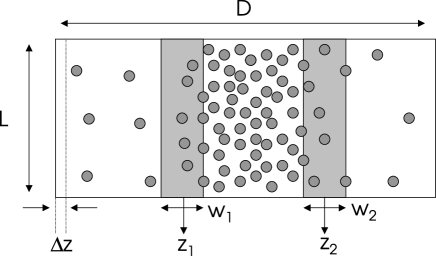
Figure 2: Schematic representation of a phase–separated colloid–polymer mixture. Colloidal particles are drawn as circles, the polymers are not shown. The colloid dense phase is centered around the middle of the box at $z=D/2$. The shaded regions represent interfaces, located around $z_{1}$ and $z_{2}$, and respective widths $w_{1}$ and $w_{2}$. See also details in text.

Before applying the block analysis method, the interfaces in the configuration are isolated from the bulk regions. In doing so, we ensure that the local interface position $h(x,y)$ is not influenced by density fluctuations that occur deep inside the bulk. A schematic representation of a phase–separated configuration is shown in Fig. 2. The colloids are drawn as circles, the polymers are for clarity not shown.

The use of periodic boundary conditions leads to the formation of two interfaces. The interface regions are shaded gray in Fig. 2. One interface is located around $z_{1}$, the other around $z_{2}$. The respective widths are $w_{1}$ and $w_{2}$. To obtain numerical values for the interface locations and the widths, we divide the box into $N$ equal slabs perpendicular to the $\hat{z}$ direction. Each slab has area $L^{2}$ and width $\Delta z=D/N$. The colloid density profile along the $\hat{z}$ direction is now estimated by $\rho(z)=n/(\Delta zL^{2})$, with $n$ the number of colloids in the slab centered around $z$. A similar expression holds for the polymer density profile.

Figure 3: Profile of the colloid packing fraction (solid line) and polymer packing fraction (dashed line) along the elongated $\hat{z}$ direction at $\eta_{\rm p}^{\rm r}=1.1$. The profiles were obtained from a single configuration of size $\{L=60;D=120\}$. This corresponds to approximately 13,000 colloidal particles and 130,000 polymers. The number of slabs used in calculating the profiles was $N=100$. The horizontal dotted lines represent the bulk packing fractions obtained from histogram reweighting taken from Table 1. Arrows mark the bounds of the interface regions obtained by fitting to Eq.(8). Each interface region contains around 2000 colloids and 16,000 polymers.

Typical profiles for the AO model obtained in this way are shown in Fig. 3, with density converted to packing fraction. The solid line shows the colloid packing fraction as a function of $z$, the dashed line shows the corresponding polymer packing fraction. Important in these profiles is the height of the plateaus, which must be in agreement with the bulk packing fractions obtained from histogram reweighting. The latter values are listed in Table 1, and represented in Fig. 3 by the horizontal lines. We observe that the plateaus are in good agreement with Table 1, indicating that the configuration has reached thermal equilibrium.

Next, we fit the hyperbolic tangent of Eq.(8) to the profiles of Fig. 3. We emphasize that these are two–parameter fits in the width and interface location only. For the coexistence densities, one uses the values of the bulk phase diagram. To measure the location $z_{1}$ of the left interface and its width $w_{1}$, the range of the fit is set to $0<z<D/2$. For the right interface, the appropriate range is $D/2<z<D$. One still has the choice to fit to the colloid profile, or to the polymer profile. Since the number of polymers is much larger than the number of colloids, a fit to the polymer profile seems to be the most sensible. To ensure that the entire interface region is captured, we multiply the width $W$ obtained from the fit by a factor $\alpha>1$. The bounds of the interface region are thus written as:

$$z_{\pm}=z_{0}\pm\alpha W.$$ (16)

As an illustration, the best fit parameters for the polymer profile in Fig. 3 are $\{z_{0}=36.5;W=2.37\}$ (left) and $\{z_{0}=83.5;W=2.86\}$ (right). The corresponding bounds are marked by the arrows in Fig. 3, where we used $\alpha=3$.

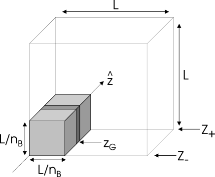
Figure 4: Schematic illustration of the block analysis method. The interface region is divided into rectangular segments. In each segment, the Gibbs surface defines a local interface position $z_{G}$. See details in text.

Figure 5: Schematic density profile (colloid or polymer) along the $\hat{z}$ direction in a single segment. The Gibbs surface is located at $z_{G}$, such that areas A and B are equal.

IV.2 Block analysis

Having identified the interface regions in a single configuration, the next task is to extract the local interface position $h(x,y)$. For this we use the block analysis method, which is schematically illustrated in Fig. 4. The figure shows one of the interface regions, and contains all those particles whose $z$ coordinates are between $z_{-}<z<z_{+}$. Note that in Fig. 4, the elongated $\hat{z}$ direction points into the plane of the paper. The interface region is split up into rectangular segments of size $(L/n_{\rm B})\times(L/n_{\rm B})\times(z_{+}-z_{-})$. Here, the parameter $n_{\rm B}$ is an integer called the block factor. The total number of segments thus equals $n_{\rm B}^{2}$. An example of one such segment is also shown in Fig. 4.

We now assign a local interface position $z_{G}$ in each segment, in spirit of the Gibbs surface. To this end, we assume that the colloid (polymer) density profile $\rho_{s}(z)$, along the $\hat{z}$ direction in a single segment, is similar to Eq.(8). The Gibbs surface runs perpendicular to the $\hat{z}$ direction, such that the shaded regions in Fig. 5 have equal area. For the areas A and B we may write

$$A=\int_{z_{-}}^{z_{G}}\rho_{s}(z){\rm d}z-\rho_{A}(z_{G}-z_{-}),$$ (17)

$$B=\rho_{B}(z_{+}-z_{G})-\int_{z_{G}}^{z_{+}}\rho_{s}(z){\rm d}z,$$ (18)

with $\rho_{A}$ and $\rho_{B}$ the density of the colloids (polymers) in the vapor and liquid phase, respectively. Equating the above two expressions, and multiplying by the lateral area of a single segment, we obtain

$$n(n_{\rm B}/L)^{2}=\rho_{A}(z_{G}-z_{-})+\rho_{B}(z_{+}-z_{G}),$$ (19)

with $n$ the number of colloids (polymers) in the segment. This equation is easily solved for $z_{G}$, because $\rho_{A}$ and $\rho_{B}$ are known from the phase diagram. One attractive feature of Eq.(19) is that the precise form of the density profile need not be specified. This is also required, if the short wavelength limit is to be probed. Large block factors $n_{\rm B}$ must then be used, and the number of particles in a single segment will predominantly be zero or one. Obviously, with such low numbers, a smooth profile cannot be defined in any case. We emphasize that by using Eq.(19), two estimates for $z_{G}$ may be obtained: one determined by the number of colloids, and one by the number of polymers. Note also that $z_{G}$ may well be located outside the region bounded by $z_{-}$ and $z_{+}$.

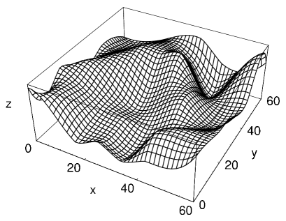
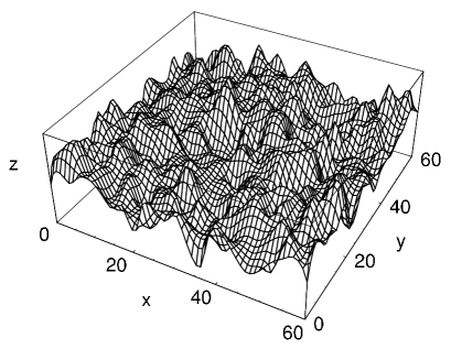
Figure 6: Influence of the block factor $n_{\rm B}$ on the local interface position $h(x,y)$. Each of the above $h(x,y)$ was extracted from the same AO configuration at $\eta_{\rm p}^{\rm r}=1.1$ and box size $\{L=60;D=120\}$. The top frame shows $h(x,y)$ obtained using $n_{\rm B}=8$, and the lower frame using $n_{\rm B}=24$.

Figure 7: Capillary amplitudes, calculated using Eq.(4) and Eq.(5), for several values of the block factor $n_{\rm B}$. The data were obtained in simulations of the AO model at $\eta_{\rm p}^{\rm r}=1.2$ and box size $\{L=60;D=120\}$. Averages over approximately 100 configurations were taken. The lines at low $q$ represent the CWT prediction of Eq.(7), with $\gamma$ taken from Table 1 and no other free parameters. For clarity, each data set has been multiplied by $n_{\rm B}$.

Figure 8: Capillary amplitudes obtained using several values of $\alpha$ in Eq.(16) as indicated. The straight line represents the CWT form of Eq.(7), with $\gamma$ taken from Table 1. The spectra were measured at $\eta_{\rm p}^{\rm r}=1.2$ and box size $\{L=60;D=120\}$. For clarity, the data have been smoothed.

Figure 9: Capillary amplitudes obtained using the polymers (triangles) and the colloids (circles) in Eq.(19). The straight line is the CWT form of Eq.(7), with $\gamma$ taken from Table 1. The spectra were measured at $\eta_{\rm p}^{\rm r}=1.2$ and box size $\{L=60;D=120\}$.

IV.3 Influence of parameters

The local interface position, as defined in the previous section, thus depends on three adjustable parameters, namely: (1) the block factor $n_{\rm B}$, (2) $\alpha$ in Eq.(16), and (3) whether $n$ in Eq.(19) is taken to be the number of colloids or the number of polymers. It is important to determine the sensitivity of the results to these parameters.

The influence of the block factor is discussed first. Here, we use $\alpha=3$, and $n$ in Eq.(19) is taken to be the number of colloids. The local interface according to our method is not defined in continuous space, but on a grid of lattice spacing $L/n_{\rm B}$, see Fig. 4. The indices $(n,m)$ in the summation of Eq.(II.1) can therefore run up to $n_{\rm B}/2$ only. As a result, the shortest wavelength that can be sampled equals $a=2L/n_{\rm B}$, or alternatively ${\Lambda_{\rm max}}=\pi n_{\rm B}/L$. One may therefore conceive $n_{\rm B}$ as a filter: via $n_{\rm B}$, all capillary modes with $q>{\Lambda_{\rm max}}$ are effectively filtered out. The effect in real–space is illustrated in the snapshots of Fig. 6. The AO configuration from which the local interface position is extracted, is the same in both snapshots, but $n_{\rm B}$ is varied. For small $n_{\rm B}$, only long–wavelength variations are visible. For larger values, short–wavelength features become visible, and the interface appears rougher. The effect of $n_{\rm B}$ in Fourier–space is shown in Fig. 7. Here, we measured the Fourier amplitudes as a function of $q$, for several values of $n_{\rm B}$. By increasing $n_{\rm B}$, the range of the data can be extended to larger values of $q$, but otherwise the spectra are unaffected. In particular, note that the spectra for $q\to 0$ are well described by the CWT prediction of Eq.(7), irrespective of $n_{\rm B}$.

Next, $\alpha$ is varied at fixed block factor $n_{\rm B}=64$, with $n$ in Eq.(19) again being the number of colloids. This result is shown in Fig. 8. For $\alpha=5$, the bounds $z_{\pm}$ lie deep inside the bulk, so considering larger values is not sensible. For small $q$, we observe that the spectra are rather insensitive to $\alpha$ and, moreover, in good agreement with Eq.(7). For $q\approx 0.2$ and above, systematic deviations become visible.

Finally, Fig. 9 shows the effect of using the polymers to determine $z_{G}$ in Eq.(19), instead of the colloids. Here, $n_{\rm B}=64$ and $\alpha=3$ were used. The agreement with Eq.(7) is again demonstrated for $q\to 0$, but at higher values deviations become visible. Note that $L^{2}\langle C^{2}\rangle$ deviates from the CWT behavior at low $q$ towards larger values. This already indicates that $\gamma(q)<\gamma(0)$ for all nonzero $q$, see Eq.(14).

In summary, the block factor $n_{\rm B}$ does not influence the capillary spectrum in any significant way; it merely sets the range in $q$ that can be sampled. In contrast, $\alpha$ in Eq.(16), and $n$ in Eq.(19), do affect the spectrum, but only at relatively large values of $q$.

V Results

We now proceed with presenting our main results, whereby the long and short wavelength limit of the capillary wave spectrum are treated separately.

Figure 10: Correlation time $\tau$ of the amplitudes $A_{n0}$, as a function of the wave number $n$, for several system sizes as indicated. The correlation time is expressed in seconds of CPU time on a 2.4 GHz Pentium machine. The local interface position $h(x,y)$ was extracted from AO configurations with $\eta_{\rm p}^{\rm r}=1.1$ and using block factor $n_{\rm B}=20$.

V.1 Long wavelength limit: $q\ll 1$

As demonstrated before, the capillary spectrum in the long wavelength limit, does not depend sensitively on the parameters used to extract the local interface position. In this section, we use $\alpha=3$ in Eq.(16), and the local interface position $z_{G}$ in Eq.(19), is determined via the colloids. To properly model long wavelength capillary modes, large system sizes are required. An important issue is then the correlation time $\tau$ of these modes. It is well–known that $\tau$ increases strongly with the size of the simulation box, such that extensive simulations are required Werner et al. (1997). For the AO model, this is illustrated in Fig. 10, where $\tau$ is plotted, for several system sizes. The data were obtained by measuring the amplitudes $A_{n0}(t)$, given by Eq.(4), at evenly spaced times $t$, with wave number $n\geq 1$. From the decay of the autocorrelation function, $\tau$ was obtained Müller-Krumbhaar and Binder (1973); Newman and Barkema (1999). As expected, $\tau$ decreases with the wave number. In a simulation, the important quantity is the correlation time of the amplitude with the smallest wave number: $A_{10}$. It is crucial to ensure that the duration of the simulation exceeds the time that governs the decay of $A_{10}$. Fig. 10 shows that the corresponding correlation time increases strongly with the size of the system. We found that a system size of $\{L=60;D=120\}$ is sufficient to perform a long wavelength analysis of the interface. Since around 100 uncorrelated configurations are required to obtain the spectrum with reasonable accuracy, this amounts to approximately four days of CPU time.

Figure 11: Capillary spectrum of the AO model in the long wavelength limit, for several values of $\eta_{\rm p}^{\rm r}$ as indicated (note the double logarithmic scale). Lines represent the CWT form given by Eq.(7). All spectra were obtained using box size $\{L=60;D=120\}$ and block factor $n_{\rm B}=100$.

The capillary amplitudes are shown in Fig. 11, for several values of $\eta_{\rm p}^{\rm r}$. Also included in the figure is the CWT form of Eq.(7), with $\gamma$ taken from Table 1, and no other adjustable parameters. We observe that CWT is confirmed for all values of $\eta_{\rm p}^{\rm r}$ considered by us, up to $q_{\rm S}\approx 0.2$, corresponding to a length scale of around 15 colloid diameters.

Next, interface broadening is considered. First, note that the logarithmic dependence of $W$ on $L$, see Eq.(13), was already confirmed by us in Ref. Vink and Horbach, 2004a (for $\eta_{\rm p}^{\rm r}=1.1$), but with a factor of two discrepancy in the definition of the width. This yields an incorrect estimate of the interfacial tension. If, however, this error is accounted for, a fit to the data yields $\gamma=0.109\pm 0.004$. The deviation from histogram reweighting is around four percent, see Table 1.

Figure 12: Capillary width $W_{\rm cw}^{2}$ as a function of the block factor (note the logarithmic $n_{\rm B}$ scale). The data were obtained using box size $\{L=60;D=120\}$. Averages over approximately 100 configurations were taken. The lines represent Eq.(20), with $\gamma$ taken from Table 1, and $C$ obtained by fitting to the lowest few $n_{\rm B}$ values.

An alternative method to study interface broadening, is to vary the coarse graining length $a$ at fixed $L$, and use Eq.(12) to obtain the interfacial tension. To use this method, a single set of configurations, obtained for one value of $L$, is sufficient. For the coarse graining length, we may write $a\propto 1/n_{\rm B}$, so Eq.(12) becomes:

$$W_{\rm cw}^{2}=\frac{1}{2\pi\gamma}\ln(n_{\rm B}/C),$$ (20)

with $n_{\rm B}$ the block factor and $C$ a constant. In this approach, the local interface position $h(x,y)$ needs to be explicitly calculated. Per interface region, $n_{\rm B}^{2}$ samples $h_{i}$ of the local interface position are obtained. The variance in these samples yields an estimate for $W_{\rm cw}^{2}=\langle h_{i}^{2}\rangle-\langle h_{i}\rangle^{2}$, which is then averaged over the different configurations. In Fig. 12, we show the width $W_{\rm cw}^{2}$, as a function of $n_{\rm B}$, for a number of different $\eta_{\rm p}^{\rm r}$. The figure strikingly illustrates the broadening of the interface as the grid, on which the interface is studied, becomes finer, and more capillary modes are taken into account. For small $n_{\rm B}$, the broadening is in good agreement with Eq.(20), shown by the lines in Fig. 12. Here, $\gamma$ was taken from Table 1, and $C$ was obtained by fitting. For large $n_{\rm B}$, deviations become visible. The range of validity varies from $n_{\rm B}\approx 4$ ($\eta_{\rm p}^{\rm r}=0.9$) to $n_{\rm B}\approx 8$ ($\eta_{\rm p}^{\rm r}=1.2$). The corresponding wavelength is approximately $8-15$ colloid diameters, or equivalently $q_{\rm S}\approx 0.2-0.3$.

V.2 Short wavelength limit: $q\gg 1$

Figure 13: Capillary amplitudes for several values of $\alpha$ as indicated. Here, the colloids were used in Eq.(19) to determine $z_{G}$. The line at low $q$ is the CWT prediction of Eq.(7). The data were obtained in simulations of the AO model at $\eta_{\rm p}^{\rm r}=1.0$, using box size $\{L=20,D=40\}$. Also shown is the static structure factor $S(q)$ of the bulk colloidal liquid. Note the double logarithmic scale.

Figure 14: The analogue of Fig. 13, but using the polymers in Eq.(19) to extract the local interface position.

We now turn to the short wavelength limit of the capillary spectrum. In this case, both the parameter $\alpha$ in Eq.(16), as well as the precise choice (colloids or polymers) for $n$ in Eq.(19), become important. To illustrate the effect, we show in Fig. 13 and Fig. 14, the capillary amplitudes for several values of $\alpha$, at $\eta_{\rm p}^{\rm r}=1.0$. The data in Fig. 13 were obtained using the Gibbs surface defined by the colloids as local interface position. In Fig. 14, the Gibbs surface defined by the polymers was used. In both figures, the line at small $q$ represents the CWT form of Eq.(7). Also shown in Fig. 13, is the static structure factor $S(q)$ of the bulk colloidal liquid (multiplied by a factor of 30).

One important observation is that, for $\alpha$ sufficiently high, the local Gibbs surface defined by the colloids and the polymers, both reproduce the expected CWT result for $q\to 0$. Note also that, compared to Fig. 11, the system size is now much smaller, so the agreement with Eq.(7) is not as convincingly demonstrated as before.

More importantly, we observe in Fig. 13, that for $q_{\rm T}\approx 1.2$ and above, the capillary wave amplitudes essentially follow the static structure factor. This illustrates the point made earlier, namely that, for high $q$, the capillary spectrum is determined by the most dominant bulk fluctuations. The same effect is visible in Fig. 14, where we recall that, in the AO model, the polymers are ideal (hence no structure at large $q$). Furthermore, we deduce from Fig. 13 and Fig. 14, that the limiting value $\lim_{q\to\infty}L^{2}\langle C^{2}\rangle$ is proportional to $\alpha$: in other words, proportional to the width of the slabs in Fig. 2, or consequently, the number of particles involved in calculating $L^{2}\langle C^{2}\rangle$. This is again consistent with the view that the capillary amplitudes approach the (unnormalized) static structure factor of the bulk (note that the static structure factor is usually normalized by dividing through the total number of particles).

Figure 15: Momentum dependent interfacial tension $\gamma(q)$ for the AO model, as a function of $q^{2}$, for several values of $\eta_{\rm p}^{\rm r}$ as indicated. The data were obtained using box size $\{L=60,D=120\}$, with $n$ in Eq.(19) being the number of colloids, and $\alpha=3$.

Finally, we observe that the capillary amplitudes evolve smoothly from $L^{2}\langle C^{2}\rangle\propto 1/q^{2}$ at low $q$, to $L^{2}\langle C^{2}\rangle\propto S(q)$ at high $q$. This implies, for the $q$-dependent interfacial tension, $\lim_{q\to\infty}\gamma(q)\propto 1/q^{2}$, see Fig. 15. In agreement with (most) other simulations Stecki (2001); Müller and MacDowell (2000); Milchev and Binder (2002), we observe a strong reduction in $\gamma(q)$ with increasing $q$, but no sign of a minimum.

VI Discussion and Conclusions

First, we note that our data in the long wavelength limit, are consistent with CWT. The interfacial tension, obtained from both the spectrum and the broadening of the interface, is in good agreement with previous independent estimates Vink and Horbach (2004b). This result is encouraging, because it is difficult to simulate the long wavelength limit accurately, due to the large system sizes that are required. For the AO model, we observe that CWT remains valid down to wavelengths of around 10 colloid diameters, in reasonable agreement with Ref. Aarts et al., 2004. The data in Fig. 11 and Fig. 12, also show that the deviations become more pronounced closer to the critical point (so for low values of $\eta_{\rm p}^{\rm r}$). This is in agreement with Ref. Chacón and Tarazona, 2003.

At shorter wavelengths, CWT gradually breaks down. We observe a sharp reduction in $\gamma(q)$, followed by an asymptotic decay of the form $\gamma(q)\propto 1/q^{2}$. In the asymptotic regime, $\gamma(q)$ is essentially determined by the static structure factor, see Fig. 13 and Fig. 14. The form of $\gamma(q)$ shown in Fig. 15, is consistent with most other simulations Stecki (2001); Müller and MacDowell (2000); Milchev and Binder (2002) (an exception is Ref. Chacón and Tarazona, 2003, in which an entirely different definition of the local interface position is used).

However, the problem involved in our analysis (as well as in related previous work) is that the concept of a local interface in terms of the Gibbs surface becomes questionable as the considered lateral length scale becomes smaller and smaller. Since in the theory of Mecke and Dietrich Mecke and Dietrich (1999) a somewhat different approach is used, it is not clear if there is a real contradiction between our results and their treatment (note also that we work with a model exhibiting strictly short range forces, while Ref. Mecke and Dietrich, 1999 employs long range van der Waals forces). Our results clearly point towards the need of a different analysis of simulations (and experiments) suitable to consider the interplay of bulk and interfacial fluctuations on intermediate and short length scales. Note that the pronounced size–dependence of the simulated interfacial profiles makes our analysis in terms of the intrinsic interfacial width rather meaningless as well, and this complicates a direct comparison of our data to theoretical studies Brader et al. (2003); Moncho-Jordá et al. (2004).

The problem that the concept of a local interface becomes ill-defined on the microscopic scale (correlation lenght in the bulk, or interparticle distances in the fluid in the extreme case) also calls into question the extent to which the concept of a wavevector–dependent interfacial tension $\gamma(q)$ is really meaningful. Fig. 13 and Fig. 14 indicate that one must be careful with the choice of the parameter $\alpha$, and only for $\alpha\gg 1$ do we observe convergence of the data for small $q$. At large $q$, however, the dependence on $\alpha$ is very pronounced (reflecting essentially the number of particles used in the calculation). Nevertheless, whatever the value of $\alpha$, the data always follow the static structure factor in the bulk, see Fig. 13. This finding is sensible because if one probes the interface on such small scales, the local structure reflecting how the particles in the fluid are stacked, should show up in the analysis.

It remains a challenge for future work to try to extract from simulations the precise analog of the structure factor obtained in scattering experiments Doerr et al. (1999); Fradin et al. (2000); Mora et al. (2003); Li et al. (2004) and to conduct such an analysis with the present data.