On X-ray-singularities in the f-electron spectral function of the Falicov-Kimball model

Abstract

The f-electron spectral function of the Falicov-Kimball model is calculated within the dynamical mean-field theory using the numerical renormalization group method as the impurity solver. Both the Bethe lattice and the hypercubic lattice are considered at half filling. For small U we obtain a single-peaked f-electron spectral function, which –for zero temperature– exhibits an algebraic (X-ray) singularity ($|\omega|^{-\alpha}$) for $\omega\rightarrow 0$. The characteristic exponent $\alpha$ depends on the Coulomb (Hubbard) correlation U. This X-ray singularity cannot be observed when using alternative (Keldysh-based) many-body approaches. With increasing U, $\alpha$ decreases and vanishes for sufficiently large U when the f-electron spectral function develops a gap and a two-peak structure (metal-insulator transition).

I Introduction:

One of the simplest lattice models for strongly correlated electron systems, the Falicov-Kimball model (FKM) FalicovKimball69 , consists of two types of spinless electrons, delocalized band ($c$-) electrons, localized $f$-electrons and a local Coulomb (Hubbard) interaction between $c$- and $f$-electron at the same site. The FKM Hamiltonian reads

$$H = -\sum_{ij}t_{ij}c^{\dagger}_{i}c_{j}+\varepsilon_{c}\sum_{i}c^{\dagger}_{i}c_{i}+\varepsilon_{f}\sum_{i}f^{\dagger}_{i}f_{i}$$ (1)

$$+U\sum_{i}c^{\dagger}_{i}c_{i}f^{\dagger}_{i}f_{i}\;\;.$$

where $\varepsilon_{f}$ denotes the one-particle energy of the $f$-electrons, $\varepsilon_{c}$ the band center of the $c$-electrons, $t_{ij}$ the c-electron hopping between site $i$ and $j$ and U the Coulomb (Hubbard) correlation. This model can be interpreted as a simplified version of the one-band Hubbard model Hubbard64 where $c$ and $f$ translates to the label of the different spin orientations, and the hopping term for the $f$-spin type is set to zero. The FKM was originally introduced as a model for metal-insulator and valence transitions FalicovKimball69 . It can also be interpreted as a model for crystallization (identifying the ”heavy” $f$-particles with the nuclei, the $c$-particles with the electrons and for $U<0$) KennedyLieb86 . Furthermore, the FKM is of interest for academic reasons, because it is the simplest, non-trivial lattice model for correlated electron systems, for which certain exact results are available; for a recent review see Ref. FreericksZlatic03, . Therefore, the FKM may serve as a test case and benchmark for any many-body method and approximation, because such a method can also be applied to the FKM and comparisons of the approximate and the available exact results may help to judge the value and possible limitations of such many-body techniques.

Brandt and Mielsch BrandtMielsch89 solved the FKM exactly in the limit of infinite spatial dimensions, $d\rightarrow\infty$ MetznerVollhardt89 , by mapping the problem onto an effective single site subject to a complex bath. Thereby, the complex bath field mimics the dynamics of the surrounding electrons on the lattice. Since the local $f$-electron number is conserved, $[H,f^{\dagger}_{i}f_{i}]=0$, the $c$-electron problem is solved independently from the dynamics of the $f$-electrons which are static. However, the presence or absence of an $f$-electron on the effective site induces a significant change for the conduction electrons: the presence of an $f$-electron switches on an additional scattering potential $U$ for the conduction electrons. Brandt and MielschBrandtMielsch89 were able to derive an exact, explicit expression for the self-energy of the $c$-electrons $\Sigma_{c}(z)$, which is a functional of the local $c$-electron Green function and the (fixed) local $f$-electron occupation numbers. This functional is essentially equivalent to that obtained in the Hubbard-III-approximation of the Hubbard modelHubbard64 , i.e. this approximation becomes exact for the $c$-electron self-energy of the FKM in the limit $d\rightarrow\infty$.

But despite the conservation of the $f$-electron occupation, the $f$-electrons have a highly non-trivial dynamics. For $U=0$ the f-electron spectral function is simply a delta-function, but for finite $U$ the spectral function broadens due to the interaction with the fluctuating $c$-electrons. The $f$-electron Green function $G_{f}(z)$ of the FKM is much more involved and less trivial than the $c$-electron Green function $G_{c}$, in particular a Hubbard-III-type self-energy functional does not become exact for the $f$-electrons. Even for large dimensions, where the mapping on an effective impurity problem holds, it is not possible to derive an explicit analytical expression for the $f$-electron self-energy functional $\Sigma_{f}$. On the contrary, the evaluation of $\Sigma_{f}$ is nearly as complicated as the self-energy of the full Hubbard model. For $d\rightarrow\infty$, the first explicit numerical evaluation of $G_{f}$ (or the $f$-electron spectral function $\rho_{f}$, respectively) was performed by Brandt and UrbanekBrandtUrbanek92 . They started from a nonequilibrium, Keldysh based many-body formalism using a discretization along the Kadanoff-Baym contour and a subtle analytical continuation to obtain the dependence on real frequency numerically. Only relatively few explicit results were presented in Ref. BrandtUrbanek92, . Therefore, this Keldysh based analysis was repeated very recently by Freericks et al.FreericksZlatic2004 presenting much more explicit results and investigating also the accuracy of the results by checking sum rules and the dependence on the numerical discretization and the cutoff in the time integrals.

On the other hand, it is clear that the problem to calculate the $f$-electron Green function $G_{f}(\tau)=-\langle T(f_{i}(\tau)f^{\dagger}_{i})\rangle$ must be related to the X-ray threshold problem, because the creation of a core hole, with which the conduction electrons then interact, is related to the creation of an f-electron at a certain time as pointed out by Si et al. SiKotliarGeorges1992 and Möller et al. MoellerRuckensteinSchmittRink1992 As in the X-ray problem the non-interacting Fermi sea of $c$-electrons has to relax into an orthogonal ground state through an infinite cascade of particle-hole excitations after an $f$-electron has been added to the system by $f^{\dagger}_{i}$. However, though the relation to the X-ray problem is known, no observations of the characteristic X-ray singularities were made in previous studies of $G_{f}$ for the FKM. BrandtUrbanek92 ; FreericksZlatic2004

In this paper, we apply a different method to the FKM, namely the dynamical mean-field theory (DMFT), i.e. the (exact) mapping of the $d\rightarrow\infty$ problem on an effective impurity problemBrandtMielsch89 ; Georges96 , and Wilson’s numerical renormalization group approach (NRG)Wilson75 as the impurity solver. Within this DMFT/NRG the typical X-ray singularities, in fact, occur for $G_{f}$ of the FKM. The spectral function of $G_{f}$ exhibits a power law $|\omega|^{-\alpha}$ divergence for the half-filled homogeneous solution at the chemical potential when $T\to 0$. Since the norm of the spectral function is finite, the upper limit for $\alpha$ is one: $\alpha<1$. This new finding has not been previously discussed in the existing literature on the $f$-spectral function of the FKMBrandtUrbanek92 ; FreericksZlatic2004 . The power-law scaling of the $f$-spectra is related to an infra-red problem which –due to the logarithmic discretization– can properly be resolved within the NRG. We will show that the exponent $\alpha$ is proportional to the imaginary part of the bath field. Since small frequencies correspond to a very large time scale, this X-ray threshold behavior cannot be seen in the Keldysh-contour approach by integrating the equation of motion in real time up to a finite cutoff in timeBrandtUrbanek92 ; FreericksZlatic2004 . For sufficiently high temperatures, where the X-ray singularities no longer exist, our results are in good agreement with Ref. FreericksZlatic2004, .

Our investigation can also be motivated as a test or benchmark of the different possible (numerical) many-body methods, which can be applied to the FKM (and thus to correlated electron models, in general). To resolve fine structures on a small frequency scale (around the chemical potential) the DMFT/NRG is clearly superior to the Keldysh based method. Furthermore, the numerical efforts and resources needed are smaller by magnitudes; whereas supercomputers had to be used in Ref.FreericksZlatic2004, , our results can be obtained on conventional PCs (or laptops) needing only seconds of computation time. Finally, as a byproduct we obtain also the $c$-electron Green function $G_{c}$ and self-energy $\Sigma_{c}$ within the DMFT/NRG approach, which is known independently from the exact self-energy functional. Though it is known that the NRG is slightly less accurate in the reproduction of high-frequency featuresRaasUhrigAnders2003 (just because of the logarithmic discretization and the resulting lower resolution at higher frequencies), very good agreement is obtained also for this quantity.

II Theory

II.1 Dynamical Mean Field Theory

The FKM was solved exactly for $d\rightarrow\infty$ by Brandt and Mielsch BrandtMielsch89 . Using the locality of the self-energy $\Sigma_{c}$ MuellerHartmann89 , they showed that the local conduction electron Green function for the homogeneous phase must have the form

$$G_{c}^{loc}(z) = \frac{1-n_{f}}{z+\mu-\varepsilon_{c}-\Gamma(z)}+\frac{n_{f}}{z+\mu-\varepsilon_{c}-\Gamma(z)-U}$$ (2)

since the local $f$-electron number is conserved: $[H,f^{\dagger}_{i}f_{i}]=0$. $n_{f}=\langle f^{\dagger}_{i}f_{i}\rangle$ is the average number of $f$-electrons at site $i$, and the complex dynamical field $\Gamma(z)$ contains the dynamics due to the coupling of the effective site to the remainder of the system (lattice). The local Green function $G_{c}(z)$ can also be obtained from the self-energy $\Sigma_{c}$

$$\Sigma_{c}(z) = z+\mu-\Gamma(z)-[G_{c}(z)]^{-1}$$ (3)

via Hilbert transformation

$$G_{c}^{latt}(z) = \int d\varepsilon\frac{\rho_{0}(\varepsilon)}{z+\mu-\varepsilon-\Sigma_{c}}$$ (4)

$$G_{c}^{latt}(z) = G_{c}^{loc}(z)\;\;.$$ (5)

For given $f$-occupation $n_{f}$, Eqns. (2-5) form a set of self-consistency equations from which the dynamical field $\Gamma(z)$ and the self-energy $\Sigma_{c}(z)$ can be calculated. To this end, the level position $\varepsilon_{f}$ has to be adjusted such that the average $f$-occupation is given by $n_{f}$. For a fixed total particle number $n_{tot}$ per site - $n_{tot}=n_{f}+n_{c}$ - the chemical potential is adjusted accordingly.

II.2 Dynamical Properties of the Effective Site

The effective site can also be viewed as an effective single impurity Anderson model (SIAM)Kim87 ; Jarrell92 ; Pruschke95 ; Georges96

$$H_{eff} = (\varepsilon_{c}-\mu)c^{\dagger}c+(\varepsilon_{f}-\mu)f^{\dagger}f$$ (6)

$$+\int d\varepsilon\;\varepsilon d^{\dagger}_{\varepsilon}d_{\varepsilon}+U\hat{n}_{c}\hat{n}_{f}$$

$$+\int d\varepsilon\;V\sqrt{\rho_{\mbox{\tiny eff}}(\varepsilon)}\left(d^{\dagger}_{\varepsilon}c+c^{\dagger}d_{\varepsilon\sigma}\right)\;\;.$$

with an energy dependent hybridization function $\Delta(\varepsilon)=V^{2}\rho_{\mbox{\tiny eff}}(\varepsilon)=\Im m\Gamma(\varepsilon-i0^{+})$ describing the coupling of the $c$-electron to a fictitious bath of ”conduction electrons” created by $d^{\dagger}$ with density of states (DOS) $\rho_{\mbox{\tiny eff}}(\varepsilon)$. The $f$-electron does not interact with the bath field. The hybridization strength $V$ is chosen to be constant and defined via

$$\pi V^{2} = \int d\varepsilon\,\Delta(\varepsilon)$$ (7)

and the DOS of the (fictitious) ($d$) conduction electrons is given by $\rho_{\mbox{\tiny eff}}(\varepsilon)=\Delta(\varepsilon)/(\pi V^{2})$.

Using the equation of motion for Fermionic Green functions,

$$z\ll\!\!A|B\!\!\gg(z) = \langle\{A,B\}\rangle+\ll\!\![A,H]|B\!\!\gg(z)$$ (8)

with the commutators $[c,H_{eff}]$ and $[f,H_{eff}]$, it is straightforward to derive two exact relations for the local $c$- and $f$-Green function of the effective site, $G_{c}(z)=\ll\!\!c|c^{\dagger}\!\!\gg$ and $G_{f}(z)=\ll\!\!f|f^{\dagger}\!\!\gg(z)$

$$\left(z-\varepsilon_{c}-\Gamma(z)\right)G_{c}(z) = 1+U\ll\!\!cf^{\dagger}f|c^{\dagger}\!\!\gg(z)$$ (9)

$$\left(z-\varepsilon_{f}\right)G_{f}(z) = 1+U\ll\!\!fc^{\dagger}c|f^{\dagger}\!\!\gg(z)\;\;.$$ (10)

Parameterizing the Green functions via a self-energy $\Sigma_{c/f}$, $G_{c}=[z-\varepsilon_{c}-\Gamma(z)-\Sigma_{c}(z)]^{-1}$ and $G_{f}=[z-\varepsilon_{f}-\Sigma_{f}(z)]^{-1}$, yields the exact relations

$$\Sigma_{c}(z) = U\frac{F_{c}(z)}{G_{c}(z)}$$ (11)

$$\Sigma_{f}(z) = U\frac{F_{f}(z)}{G_{f}(z)}$$ (12)

with $F_{c}(z)=\ll\!\!cf^{\dagger}f|c^{\dagger}\!\!\gg$ and $F_{f}(z)=\ll\!\!fc^{\dagger}c|f^{\dagger}\!\!\gg$. The problem to be solved is just a special case of a SIAM BullaHewsonPruschke98 with the hybridization matrix element for one spin component set to zero.

II.3 The Numerical Renormalization Group (NRG)

The Hamiltonian (6) is solved using the NRGWilson75 . The core of the NRG approach is a logarithmic energy discretization of the effective $d$-conduction band around the Fermi energy, $\omega_{n}^{\pm}=\pm D\lambda^{-n}$ and $\Lambda>1$, and a unitary transformation of the basis $d_{\omega_{n}^{\pm}\alpha\sigma}$ onto a basis such that the Hamiltonian becomes tridiagonal. The first Fermionic operator Wilson75 $b_{0\alpha\sigma}$ is defined as $b_{0}=\frac{1}{2}\sum_{n}(d_{\omega_{n}^{+}}+d_{\omega_{n}^{-}})$. Only $b_{0}$ couples directly to the impurity degrees of freedom. Eq. (6) is recasted as a double limit of a sequence of dimensionless NRG Hamiltonians:

$${\cal H}=\lim_{\Lambda\rightarrow 1^{+}}\lim_{N\rightarrow\infty}\left\{D_{\Lambda}\Lambda^{-(N-1)/2}{\cal H}_{N}\right\},$$ (13)

with $D_{\Lambda}=D(1+\Lambda^{-1})/2$, and

$${\cal H}_{N} = \Lambda^{\frac{N-1}{2}}\left[\frac{(\varepsilon_{f}-\mu)f^{\dagger}f+(\varepsilon_{c}-\mu)c^{\dagger}c}{D_{\Lambda}}\right.$$

$$+\left(\tilde{V}b^{\dagger}_{0}c+{\rm H.c.}\right)$$

$$+\left.\sum_{n=0}^{N-1}\Lambda^{-\frac{n}{2}}\xi_{n}\left\{b^{\dagger}_{n+1}b_{n}+{\rm H.c.}\right\}+\sum_{n=0}^{N}\Lambda^{-\frac{n}{2}}\eta_{n}b^{\dagger}_{n}b_{n}\right].$$

$\tilde{V}$ is related to the hybridization width $V=D_{\Lambda}\tilde{V}$

$$\pi V^{2}=\int d\varepsilon\Delta(\varepsilon)$$ (14)

while the pre-factor $\Lambda^{(N-1)/2}$ guarantees that the low-lying excitations of ${\cal H}_{N}$ are of order one for all $N$ Wilson75 . The energy dependent hybridization function $\Delta(\omega)$ determines the coefficients $\xi_{n}$ and $\eta_{n}$ Wilson75 ; BullaPruschkeHewson97 by performing the unitary transformation from the basis $d_{\omega_{n}^{\pm}}$ to $b_{n}$.

The NRG is used to calculate the spectral function of the Green function for the Fermionic operators $A$ and $B$

$$\rho_{A,B}(\omega) = \frac{1}{\pi}\Im m[G_{A,B}(\omega-i0^{+})$$ (15)

$$= \frac{1}{Z}\sum_{n,m}\left(e^{-\beta E_{n}}+e^{-\beta E_{m}}\right)A_{nm}B_{mn}$$

$$\times\delta(\omega+E_{n}-E_{m})\;\;,$$

where the matrix elements $A_{nm}=\langle n|A|m\rangle$ are calculated using an eigenbasis of the Hamiltonian $H$, $H|n\rangle=E_{n}|n\rangle$. The spectral functions of $G_{c/f}$ and $F_{c/f}$ are obtained from their Lehmann representation by broadening the $\delta$-function of the discrete spectrum on a logarithmic scale, i. e. $\delta(\omega-E)\to e^{-b^{2}/4}e^{-(\log(\omega/E)/b)^{2}}/(\sqrt{\pi}b|E|)$  BullaHewsonPruschke98 . The broadening parameter is usually chosen as $0.5<b<1$, and we used $b=0.8$. In order to minimize the broadening error, the physical Green functions are calculated indirectly using the self-energies $\Sigma_{c/f}(z)$ given by Eqs. (11) and (12) BullaHewsonPruschke98 . The self-energy $\Sigma_{c}$ is redundant at this point since it was already obtained from the self-consistency cycle Eqs. (2-5). However, it can be used to quantify the discretization error of the NRG, especially at high energies RaasUhrigAnders2003 . Since the $f$-electrons do not hybridize, only a spinless bath must be considered which makes the NRG calculations extremely fast.

III Results

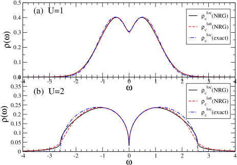
Figure 1: Spectral function of the $c$-Green function of the effective site (solid line), the lattice $c$-Green function, Eqn. (4), (dashed line) both calculated using the NRG, in comparison with the exact solution obtained from Eqns. (2-5) (dotted-dashed line) for (a) a Gaussian DOS $\rho_{0}(\varepsilon)$ and U=1 and (b) a semi-circular DOS $\rho_{0}(\varepsilon)$ and $U=2$ for $T\to 0$. NRG parameters: $\Lambda=1.6$, $N=500$, $b=0.55$.

III.1 Spectral functions for $T\to 0$

We investigate the FKM for the particle-hole symmetric case in the absence of a symmetry breaking using two different densities of states (DOS) for the unperturbed conduction electrons on the underlying lattice, namely a semi-circular DOS $\rho_{0}(\varepsilon)=\sqrt{4-(\varepsilon/t^{*})}/(2\pi t^{2})$ (Bethe lattice) and a Gaussian DOS, $\rho_{0}(\varepsilon)=\exp(-(\varepsilon/t^{*})2)/(\sqrt{\pi}t^{*})$ (hyper-cubic lattice). The energy unit will be $t^{*}$ throughout the paper. At half filling, $n_{tot}=1$, and for a given set of parameters $\mu=U/2,\varepsilon_{c}=\varepsilon_{f}=0$, we solved the Eqns. (2-5) self-consistently to determine the bath field $\Gamma(z)$. Its imaginary part $\Delta(\omega)=\Im m\Gamma(\omega-i0^{+})$ is used in the algorithm described in BullaPruschkeHewson97 to determine the parameter $\xi_{n}$ which enters the NRG of the effective site of the problem; one has $\eta_{n}=0$ in the particle-hole symmetric case for all $n$.

As mentioned before, the self-energy $\Sigma_{c}$ provided by the NRG is a redundant quantity. However, we obtain $G_{c}^{latt}(NRG)$ from (4) as well as $G_{c}^{loc}(NRG)$ via $G_{c}^{loc}(NRG)=[z+\mu-\varepsilon_{c}-\Gamma(z)-\Sigma_{c}(z)]^{-1}$ (cf. (3)) which we compare with the exact result from the self-consistency equations (2-5). Their spectral functions are plotted in figure 1 for two different values of $U$ and two different DOS $\rho_{0}(\varepsilon)$. Fig. 1(a) shows a comparison for $U=1$ using the Gaussian DOS $\rho_{0}$ while the spectral functions for the semi-circular DOS and $U=2$ are plotted in 1(b). The agreement is very good. For $|\omega|\to 0$, the three spectral functions coincide within the numerical error, a sign of a highly accurate calculation of the spectral function for low frequencies due to the equation of motion. For large frequencies, the NRG spectral functions tend to be broadened too much which also yields an overestimation of the imaginary part of the self-energy $\Sigma_{c}$. Therefore $\rho^{latt}_{c}(NRG)=\Im mG_{c}^{latt}(NRG)(\omega-i0^{+})/\pi$ turns out to be slightly smaller than $\rho^{loc}_{c}(NRG)$ for large frequencies. This error is controlled by the NRG discretization parameter $\Lambda$ and can be reduced by reducing $\Lambda$ while simultaneously increasing the number of states $N_{s}$ kept after each NRG iteration. For our calculation, we used $N_{s}=500$ and $\Lambda=1.6$. We like to emphasize that we only need to add a spin-less chain link in each NRG iteration which increases the number of states by a factor of $2$ contrary to the usual single impurity Anderson or Kondo model where $4$ states are needed to describe a new chain link which makes the NRG calculations extremely fast as mentioned before.

Two discretization errors determine the deviation of the high energy curves: the discretization errors in the determination of the NRG hopping parameters $\xi_{n}$ by averaging $\Delta(\omega)$ over the energy intervals $D[\Lambda^{-n},\Lambda^{-n+1}]$ and the artificial broadening of the $\delta$-function in the Lehmann representation of the spectral function (15). It is know that the latter is partially compensated using the equation of motionBullaHewsonPruschke98 . These systematic errors occur in all applications of the NRG as solver of the effective single-site problem in the dynamical mean field theory. However, these errors do not have any influence on the spectral properties for $|\omega|\to 0$. Here, the NRG furnishes an unprecedented resolution due to the logarithmic discretization of the energy mesh. This enables us to reveal the X-ray properties of the $f$-spectral function not visible in the previously published calculationsBrandtUrbanek92 ; FreericksZlatic2004 , because the –in principle exact– method used there requires a discretization and time cutoff in the numerical evaluation limiting the accessible resolution.

(a)

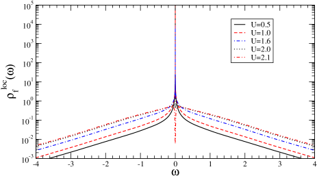
(b)

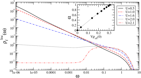
Figure 2: $f$-spectral function for different $U$ for the semi-circular $\rho_{0}(\varepsilon)$. (a) shows the spectra on a linear-log scale, (b) the same data on a log-log scale for positive frequencies. For $|\omega|\to 0$, the spectral function has an algebraic singularity: $\rho_{f}(\omega)\propto|\omega|^{-\alpha}$. The inset of (b) displays the linear dependence of $\alpha$ on the dimensionless coupling constant $g=V\rho_{\mbox{\tiny eff}}(0)$ for the metallic case $g>0$. With increasing $U$, $g$ decreases monotonically. NRG parameters as in Fig. 1

After we have established the excellent agreement between the NRG solution for the FKM and exact result for the $c$-electron spectral function, we will focus on the $f$-spectral function in the remainder of the paper. The $f$-spectral function for the FKM with semi-elliptical DOS is shown in Fig. 2 for $T\to 0$. Clearly visible in the linear-log plot 2(a) is the divergence of the spectral function for $|\omega|\to 0$, while Fig. 2(b) reveals its algebraic nature for the metallic case ($g>0$): $\rho_{f}(\omega)\propto|\omega|^{-\alpha}$. The $f$-Green function describes the response of the system to the addition or removal of an $f$-electron onto a lattice site. This process suddenly changes the Coulomb potential for the itinerant conduction electrons. Since the $f$-electron number is conserved in the absence of a $t_{ff}$-hopping matrix element, the bath conduction electrons have to relax to the new ground state under the presence of the time independent additional scattering potential in a similar way as in the X-ray edge problem RouletGavNozieres69 . This infinite cascade of particle-hole excitations generates a logarithmic slow-down which yields an algebraic singularity in the spectral function $\rho_{f}(\omega)$. The connection between these two problems is mentioned in Refs.SiKotliarGeorges1992, ; MoellerRuckensteinSchmittRink1992, , for instance. But previous calculations of the $f$-spectral functions BrandtUrbanek92 ; FreericksZlatic2004 do not reveal this feature since the method used there is based on a real time integration along Keldysh contours. In order to see the algebraic singularities, numerical integrations at $T=0$ to exponentially large time scales would have to be performed, which is not possible in practice also because of the possible accumulation of numerical errors.

The inset of Fig. 2(b) shows the dependence of the exponent $\alpha$ on the dimensionless coupling constant $g=V\rho_{\mbox{\tiny eff}}(0)=\Im m\Gamma(0-i0^{+})/(V\pi)$ at the chemical potential. With increasing $U$, $g$ is monotonically decreasing. At the same time, the exponent $\alpha$ is also reduced as can be seen in Fig. 2(b). We find a linear connection between $g$, which is implicitly $U$ dependent, and the exponent $\alpha$. A relation between $U$ and $\alpha$ was already discussed in Ref.SiKotliarGeorges1992, . There –for the (unphysical) assumption of a Lorentzian unperturbed DOS– a mapping on Nozieres’ original X-ray problemRouletGavNozieres69 ; Nozieres71 was made. But obviously the exponent $\alpha$ obtained within our DMFT/NRG treatment approaches $0$ at a critical interaction strength $U_{c}$, at which the metal-insulator transition sets in, whereas no critical $U_{c}$ is obtained in Ref.SiKotliarGeorges1992, , probably because only a single-impurity (and no selfconsitent DMFT-scheme) is considered there. Since the total spectral weight of $\rho_{f}$ is 1, the integral over a small interval around zero, on which the power law behavior is valid, must be finite, too, i. e.

$$\int_{-\eta}^{\eta}d\omega\rho_{f}(\omega) = a\int_{-\eta}^{\eta}d\omega|\omega|^{-\alpha}<1$$ (16)

Therefore, $\alpha<1$ must hold. The exponent $\alpha$ obtained by a power-law fit to the spectral function up to $|\omega|\approx 10^{-8}$ is consistent with this analytical requirement.

(a)

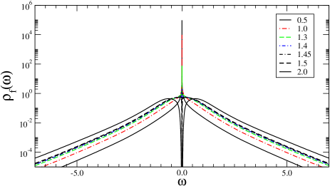
(b)

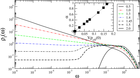
Figure 3: $f$-spectral function for different $U$ for the Gaussian DOS $\rho_{0}(\varepsilon)$. (a) shows the spectra on a linear log scale, (b) the same data on a log-log scale for positive frequencies. For $|\omega|\to 0$, the spectral function has an algebraic singularity: $\rho_{f}(\omega)\propto|\omega|^{-\alpha}$. The inset of (b) displays the linear dependence of $\alpha$ on the dimensionless coupling constant $g=V\rho_{\mbox{\tiny eff}}(0)$ of the effective site. NRG parameters as in Fig. 1

Figure 3 shows the evolution of the $f$-spectral function $\rho_{f}(\omega)$ for a Gaussian unperturbed DOS $\rho_{0}(\omega)$ as function of $U$ for the same NRG parameter as in Fig. 2. In the chosen units, the square of the effective hybridization strength, $V^{2}=0.5$ is half the size of the value for $V^{2}$ for the semi-circular DOS. Therefore, the metal-insulator transition occurs at a smaller value of $U$. Setting aside this difference and the slightly different shapes, the spectra are similar. As expected, the spectral functions also show a power law behavior for $|\omega|\to 0$.

We have also checked the basic sum rules $\rho_{f}$ has to fulfillFreericksZlatic2004 . Whereas the basic rules $\int d\omega\rho_{f}(\omega)=1,\int d\omega\rho_{f}(\omega)f(\omega)=0.5$ and $\int d\omega\rho_{f}(\omega)\omega=0$ are exactly fulfilled, the ruleFreericksZlatic2004 $\int d\omega\rho_{f}(\omega)\omega^{2}=U^{2}/4$ is slightly violated within our NRG-scheme. We obtain a proportionality to $U^{2}$ but with a larger prefactor, probably as the NRG is less accurate at higher frequencies which get a higher weight due to the $\omega^{2}$-factor under the integral.

III.2 $f$-Electron Self-energy

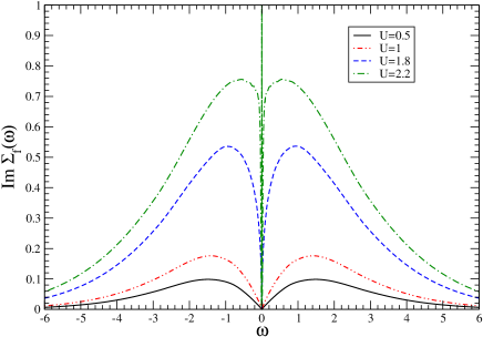
Figure 4: Imaginary part of the $f$-electron self-energy $\Im m\Sigma(\omega-i0^{+})$ for different values of $U$ and a semi-circular unperturbed DOS. The scattering rate increases with increasing $U$ as expected from Eqn. (12). Parameters as in Fig. 2.

The imaginary part of $\Sigma_{f}(\omega-i0^{+})$ is shown in Fig. 4 for 4 different values of $U$ and a semi-circular unperturbed DOS. For the metallic case, $U=0.5,1,1.8<U_{c}$, $\Im m\Sigma_{f}(\omega-i0^{+})\to 0$ for $\omega\to 0$ as expected from the suppression of scattering processes on conduction electrons. However, obviously we observe here again a non-analytic, power-law behavior. Therefore, the $f$-electron spectral function and self-energy of the FKM provides for an example and paradigm of a system exhibiting non Fermi liquid behavior. As it is well known, for a normal Fermi liquid the self-energy imaginary part has to vanish according to an $\omega^{2}$-behavior at the chemical potential. But here we have obviously no $\omega^{2}$-behavior but a non-analytic vanishing of $\Im m\Sigma_{f}(\omega)$. Via $G_{f}=[z-\varepsilon_{f}-\Sigma_{f}(z)]^{-1}$ this non-analytic self-energy behavior translates to a divergence in the spectral function for $|\omega|\to 0$. Above a critical value of the Coulomb interaction $U$, namely for $U=2.2>U_{c}$, the solution of the DMFT yields an insulating behavior, i.e. a gap in the $f$-electron spectral function. Then, the imaginary part of $\Sigma_{f}(\omega-i0^{+})$ has an additional $\delta(\omega)$ peak, i.e. there $\Sigma_{f}(\omega-i0^{+})$ has a pole at $\omega=0$, which leads to a vanishing $f$-spectral function in the energy-gap around the chemical potential. This metal insulator transition observed here is similar to the Mott-Hubbard transition occuring for the Hubbard model and for the $c$-electron spectral function of the FKM.

III.3 Finite Temperature

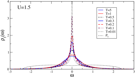
Figure 5: Evolution of the finite temperature spectral function $\rho_{f}(\omega)$ for a semi-circular DOS in the metallic phase for $U=1.5$. We truncated the $\rho(\omega)$-axis in favor of the high temperature spectral information. While for high temperatures, the peak at $\omega=0$ is rather wide, the development of the singularity is clearly visible for the smallest temperature plotted here, $T=0.01$. NRG parameters as in Fig. 1.

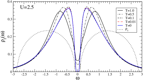
Figure 6: Evolution of the finite temperature spectral function $\rho_{f}(\omega)$ for a semi-circular DOS in the insulating phase for $U=2.5$. While for high temperatures spectral weight is still found in the gap between the two sub-bands, it is rapidly vanishing for $T<0.1$. NRG parameters as in Fig. 1.

We used a newly developed finite temperature algorithm, as described in appendix A, to calculate the NRG spectral functions which enter the Eqns. for the local self-energies, (11) and (12). Figure 5 shows the $f$-spectral function for different temperatures in the metallic phase for $U=1.5$. At high temperatures, the peak at $\omega=0$ is rather broad. Lowering the temperature, the algebraic singularity clearly gradually develops. Since we have established its existence in the normal metallic phase in the previous section, we truncated the height of the $\rho(\omega)$-axis in favor of the high temperature spectral information. These results agree nicely with those obtained recently by Freericks et. al. FreericksZlatic2004 , compare their Fig. 6. Since they obtain their spectral function at finite temperature by integration in the time domain, their spectral function is resolution limited by the largest time $t_{l}$ of the numerical integration, $\omega_{min}=1/t_{l}$. For $T\to 0$, they extrapolate $\rho_{f}(0)$ to a finite value, which is essentially displayed in the inset in Fig. 6 of Ref. FreericksZlatic2004, . However, our work shows that $\rho_{f}(\omega=0,T\to 0)\to\infty$ with a power law $\rho_{f}(\omega)\propto|\omega|^{-\alpha}$ which could not be seen in Ref. FreericksZlatic2004, because of the limited frequency resolution inherent to the method used. Figure 6 displays the evolution of the finite temperature $f$-spectral function in the insulating phase for $U=2.5$. While at higher temperature, finite spectral weight is found in the vicinity of $\omega=0$, rather rapidly a gap develops for temperatures $T<0.1$. The difference between the $T=10^{-2}$ and the $T=0$ spectral function is marginal for $|\omega|>T=10^{-2}$. This behavior is again essentially in agreement with results obtained in Ref. FreericksZlatic2004, , compare Fig. 7 in that reference.

IV Discussion and Conclusion:

We calculated the f-electron spectral function $\rho_{f}$ of the FKM at half filling in the $d\rightarrow\infty$ limit using the DMFT/NRG method. $\rho_{f}$ is strongly temperature dependent, for small values of $U$, it has a single peak structure with a power law singularity $|\omega|^{-\alpha}$ for $\omega\to 0$ at zero temperature $T=0$. For larger $U>U_{c}$, a metal-insulator (Mott-Hubbard) transition occurs and $\rho_{f}$ gets a two-peak structure with a gap at $T=0$. Therefore, the obvious connection of the FKM with the X-ray threshold problem SiKotliarGeorges1992 ; MoellerRuckensteinSchmittRink1992 has been explicitely worked out and demonstrated here. The imaginary part of the f-electron self-energy vanishes for $\omega\rightarrow 0$ for small $U<U_{c}$, but it does not follow the standard Fermi liquid $\omega^{2}$-law, but it vanishes non-analytically, i.e. one obtains non Fermi liquid behavior SiKotliarGeorges1992 , which leads to the power law singularity in $\rho_{f}$. Above the metal-insulator transition, $\alpha<0$ and the threshhold $E_{0}=f(U-U_{c})$ being a function of $U-U_{c}$ is shifted to a finite energy. At finite temperatures, precursors of the algebraic signularities are found which are cut of by thermal fluctuations below $|\omega|<T$. Furthermore, the present investigation demonstrates the strength and accuracy of the DMFT/NRG method. It is not only able to resolve low frequency or temperature features with unprecedented accuracy, it is also very efficient numerically requiring only minimal resources and computation time; typical run-times have been around 2 minutes on a Pentium M laptop.

Appendix A Calculation of the Finite Temperature Green Function using the NRG

We used a slight modification of the algorithm for finite temperature Green functions by Bulla et. al.BullaCostiVollhardt01 . Our algorithm has originally been developed for multi-band models. In this case, collecting all matrix elements which contribute to $\rho_{A,B}$ (15) at each NRG iteration and patching them together as described in Fig. 2 of Ref. BullaCostiVollhardt01, is not practical in the two-band model: the number of matrix elements exceeds rather rapidly even the memory of modern supercomputers for accurate calculations. The patching of information from different iterations, however, is a very useful concept since (i) it increases the accuracy in combination with (ii) producing additional pole positions by shifting the eigenenergies slightly through iteration. Latter helps to mimic a continuum of states.

Instead of averaging individual matrix elements for different iterations, we average different $\rho_{A,B}^{M}(\omega)$ for fixed frequency $\omega$ but different iterations $M$. The basic idea is to combine the method of Costi et. al.CostiHewsonZlatic94 with the algorithm of Bulla et. al.BullaCostiVollhardt01 . The eigenstates of iteration $M$ represent excitations on an energy scale $\omega_{M}$

$$\omega_{M} = D\frac{1+\Lambda^{-1}}{2}\Lambda^{-M/2}$$ (17)

For each iteration $M$, we define a logarithmic grid interval $I_{M}$ for $3L+1$ frequencies

$$I_{M} = \omega_{M}\times\left[\Lambda^{-1},\Lambda^{-(L-1)/L},\cdots,\Lambda_{i}=\Lambda^{(i-L)/L}\cdots,\Lambda,\cdots,\Lambda^{2}\right]$$ (18)

and evaluate $\rho_{A,B}^{M}(\omega_{M}\Lambda_{i})$ via (15) for a fixed iteration $M$. Since the information between even and odd iterations are collected separately, $I_{M}$ overlaps with the $I_{M-2}$, i.e. $I_{M}\cap I_{M-1}=\omega_{M}\times\left[1,\cdots,\Lambda^{2}\right]$ and $I_{M}\cap I_{M-4}=\omega_{M}\times\left[\Lambda,\cdots,\Lambda^{2}\right]$. Only the $\rho_{A,B}^{M}(\omega)$ evaluated at the frequencies $I_{M}^{\prime}=\omega_{M}\times\left[1,\cdots,\Lambda\right]$ provide accurate information. At each iteration, we add the new data points $\rho_{A,B}^{M}(\omega_{i})$ at $\omega_{i}(M)=\omega_{M}\Lambda^{(i-L)/L}$, $i\in[0,3L]$ to the previously obtained set of spectral information by

$$\rho^{\prime}_{A,B}(\omega_{i}(M)) = \left\{\begin{array}[]{l}\displaystyle\rho_{A,B}(\omega_{i}(M))\frac{\omega_{i}-\omega_{L}}{\omega_{3L}-\omega_{L}}+\rho^{M}_{A,B}(\omega_{i}(M))\frac{\omega_{3L}-\omega_{i}}{\omega_{3L}-\omega_{L}}\hskip 8.53581pt\mbox{for}\;\;i\geq L\\ \rho^{M}_{A,B}(\omega_{i}(M))\hskip 8.53581pt\mbox{for}\;\;i<L\end{array}\right.\;\;.$$ (21)

We do the same for the spectral information at the negative frequencies $-\omega_{i}(M)$. With this recursion relation, we mimic the patching of the residua since residua far away from the frequency $\pm w_{i}(M)$ will only contribute marginal through the broadening procedure. It turned out that $L=3-7$ is a good choice, and for this work, we used $L=6$. Since the spectral information $\rho^{N}_{A,B}(\omega_{i}(N))$ for $i=0,\ldots,L-1$ is not very reliable for the last NRG iteration $N$, we drop these $L$ frequencies.

The major advantage of this new algorithm is that any temperature dependent spectral function can be calculated on the fly. There is no need for storage of information of previous iterations other than the spectral function $\rho_{A,B}(\omega)$ itself. We also use two different broadening functions

$$\delta(\omega-E) \to \left\{\begin{array}[]{lcr}\displaystyle e^{-b^{2}/4}e^{-(\log(\omega/E)/b)^{2}}/(\sqrt{\pi}b|E|)&\mbox{for}&|E|\geq L_{w}T\\ \displaystyle\frac{1}{\pi}\frac{L_{T}T}{(\omega-E)^{2}+(L_{T}T)^{2}}&\mbox{for}&|E|<L_{w}T\end{array}\right.$$ (24)

depending whether the pole position $E$ is larger than a multiple of the temperature $T$, $E\geq L_{w}T$ or $E<L_{w}T$. $L_{w}$ is a constant of the order of $1$ as suggested in the literature BullaCostiVollhardt01 . The parameter $L_{T}$ controls the width of the Lorentzian on an energy scale of $T$. Here, we used $L_{w}=0.3$ and $L_{T}=0.1$. Since the iteration $M$ also represents a characteristic temperature scale Wilson75 , we only include spectral information up to iterations CostiHewsonZlatic94 for which $\omega_{M}>L_{iter}T$ , where we chose $L_{iter}=0.1$.

References

- (1) L. M. Falicov and J. C. Kimball, Phys. Rev. Lett. 22, 997 (1969).
- (2) J. Hubbard, Phys. Roy. Soc. A 281, 401 (1964).
- (3) T. Kennedy, E. Lieb, Physica A 138, 320 (1986)
- (4) J. Freericks, V. Zlatic, Rev. Mod. Phys. 75, 1333 (2003)
- (5) U. Brandt and C. Mielsch, Z. Phys. B 75, 365 (1989).
- (6) W. Metzner, D.Vollhardt, Phys. Rev. Lett. 62, 324 (1989)
- (7) U. Brandt and M. P. Urbanek, Z. Phys. B 22, 297 (1992).
- (8) J. K. Freericks, V. M. Turkowski, and V. Zlatic, preprint, cond-mat 0407411 (2004).
- (9) Q. Si, G. Kotilar and A. Georges, Phys. Rev. B, 46, 1261 (1992)
- (10) G. Möller, A. Ruckenstein and S. Schmitt-Rink, Phys. Rev. B, 46, 7427 (1992)
- (11) A. Georges, G. Kotliar, W. Krauth, and M. J. Rozenberg, Rev. Mod. Phys. 68, 13 (1996)
- (12) K. G. Wilson, Rev. Mod. Phys. 47, 773 (1975).
- (13) C. Raas, G. S. Uhrig, and F. B. Anders, Phys. Rev. B 69, 041102(R) (2003).
- (14) E. Müller-Hartmann, Z. Phys. B. 76, 211 (1989).
- (15) C. I. Kim, Y. Kuramoto, and T. Kasuya, Solid State Commun. 62, 627 (1987).
- (16) M. Jarrell, Phys. Rev. Lett. 69, 168 (1992).
- (17) T. Pruschke, M. Jarrell, and J. K. Freericks, Adv. in Phys. 42, 187 (1995).
- (18) R. Bulla, A. C. Hewson, and T. Pruschke, J. Phys.: Condens. Matter 10, 8365 (1998).
- (19) R. Bulla, T. Pruschke, and A. C. Hewson, J. Phys.: Condens. Matter 9, 10463 (1997).
- (20) B. Roulet, J. Gavoret, and P. Nozieres, Phys. Rev. 178, 1072 (1969).
- (21) R. Bulla, T. A. Costi, and D. Vollhardt, Phys. Rev. B 64, 045103 (2001).
- (22) T. Costi, A. C. Hewson, and V. Zlatic, J. Phys.: Condens. Matter 6, 2519 (1994).
- (23) M. Combescot, P. Nozieres, J. Physique (Paris) 32, 913 (1971)