Temperature Chaos and Bond Chaos in the Edwards-Anderson Ising Spin Glasses :
Domain-Wall Free-Energy Measurements

Abstract

Domain-wall free-energy $\delta F$, entropy $\delta S$, and the correlation function, $C_{\rm temp}$, of $\delta F$ are measured independently in the four-dimensional $\pm J$ Edwards-Anderson (EA) Ising spin glass. The stiffness exponent $\theta$, the fractal dimension of domain walls $d_{\rm s}$ and the chaos exponent $\zeta$ are extracted from the finite-size scaling analysis of $\delta F$, $\delta S$ and $C_{\rm temp}$ respectively well inside the spin-glass phase. The three exponents are confirmed to satisfy the scaling relation $\zeta=d_{\rm s}/2-\theta$ derived by the droplet theory within our numerical accuracy. We also study bond chaos induced by random variation of bonds, and find that the bond and temperature perturbations yield the universal chaos effects described by a common scaling function and the chaos exponent. These results strongly support the appropriateness of the droplet theory for the description of chaos effect in the EA Ising spin glasses.

In randomly frustrated systems such as spin glasses, directed polymer in random media (DPRM) and vortex glasses, the equilibrium ordered state could be completely reorganized by an infinitesimally small change in environment McKayBerker82 ; Kitatani86 ; BrayMoore87 ; Ritort94 ; HuseKo97 ; Nifle98 ; SalesYoshino02b . This curious property called chaos effect has attracted much attention since it was found in 1980s McKayBerker82 . Especially, chaos induced by temperature variation (temperature chaos) is now of great interest because of its potential relevance for rejuvenation caused by temperature variation Rejuvenation . However, the issue of temperature chaos still remains far from being resolved. In particular, concerning low-dimensional Edwards-Anderson (EA) Ising spin glass models, the situation is very controversial because numerical studies so far done provide the evidence both for and against temperature chaos Nifle98 ; HuseKo97 ; BilloireMarinari00 ; HukushimaIba02 ; AspelmeierBray02 .

In the present work, we examine temperature chaos by numerical measurements of the domain wall free-energy $\delta F$, the difference in the free-energy between the system with the periodic boundary condition (BC) and that with the anti-periodic BC. This $\delta F$ relates to the effective coupling $J_{\rm eff}$ between the two boundary spins $S_{\rm L}$ and $S_{\rm R}$ (see Fig. 1) as $J_{\rm eff}=-\delta F/2$ BrayMoore84 ; McMillan85 . We find $\delta F$ of each sample exhibits oscillations along the temperature axis providing direct evidence of the temperature chaos. Furthermore, we find from simultaneous observations of the domain wall energy $\delta E$ and so entropy $\delta S$ that $\delta E$ and $T\delta S$ are large but they cancel with each other in the leading order to yield significantly small $\delta F=\delta E-T\delta S$. Such intriguing behavior is indeed predicted by the droplet theory DropletTheory . For a quantitative check of the droplet theory we focus on the anticipated scaling relation

$$\zeta=d_{\rm s}/2-\theta$$ (1)

derived from it, where the stiffness exponent $\theta$ is extracted from $\sigma_{F}\sim L^{\theta}$, the fractal dimension of domain walls $d_{\rm s}$ from $\sigma_{\rm S}\sim L^{d_{\rm s}/2}$, and the so called chaos exponent $\zeta$ from $C_{\rm temp}(L,T,T+\Delta)\sim f(L(\Delta T)^{-1/\zeta})$. Here $\sigma_{F}$ and $\sigma_{S}$ are the standard deviations of $\delta F$ and $\delta S$, respectively, and $C_{\rm temp}$ is the correlation function of $\delta F$’s defined by Eq.(4) below and $f(x)$ is a certain scaling function. We find the three fundamental exponents thus extracted indeed satisfy Eq. (1) well inside the spin-glass phase whose thermodynamic properties are dominantly governed by the $T=0$ fixed point.

Figure 1: Model for the boundary flip MC.

We also study bond chaos by measuring how $\delta F$ varies with changes in couplings. The result evidently shows the existence of bond chaos. Moreover, the scaling analysis of two correlation functions associated with temperature and bond perturbations reveals quantitatively that not only the chaos exponent but also the scaling function are common to both the perturbations. This universal aspect of chaos effect anticipated from the droplet theory DropletTheory is also observed in the Migdal-Kadanoff spin glasses BanavarBray87 ; NifleHilhorst92 and the DPRM SalesYoshino02b . All of our numerical results, particularly the quantitative check of Eq. (1), are strong evidence not only for the existence of chaos in the EA Ising spin glasses but also for the appropriateness of the droplet theory for its description.

The boundary flip MC method— Let us first describe the boundary flip MC method Hasenbusch93 ; Hukushima99 which enables us to measure the domain-wall free-energy. We consider a model which consists of Ising spins on a $d$-dimensional hyper-cubic lattice of $L^{d}$ and two boundary Ising spins $S_{\rm L}$ and $S_{\rm R}$ (see Fig. 1). The usual periodic BC is applied for the directions along which the two boundary spins do not lie. The Hamiltonian is ${\cal H}=-\sum_{\langle ij\rangle}J_{ij}S_{i}S_{j}$, where the sum is over all the nearest neighboring pairs including those consisting of one of the two boundary spins and a spin on the surfaces of the lattice. In our boundary flip MC simulation, the two boundary spins are also updated according to a standard MC procedure. For each spin configuration simulated, we regard the BC as periodic (anti-periodic) when $S_{\rm L}$ and $S_{\rm R}$ are in parallel (anti-parallel). Since the probability $P_{\rm P(AP)}(T)$ for finding the periodic (anti-periodic) BC is proportional to $\exp[-F_{\rm P(AP)}(T)/T]$, where $F_{\rm P(AP)}(T)$ is the free-energy with the periodic (anti-periodic) BC, we obtain, with $P_{\rm AP}=1-P_{\rm P}$,

$$\delta F(T) \equiv F_{\rm P}(T)-F_{\rm AP}(T)$$ (2)

$$= -k_{\rm B}T\{\log[P_{\rm P}(T)]-\log[1-P_{\rm P}(T)]\}.$$

We also measure the thermally averaged energy $E_{\rm P(AP)}(T)$ when the two boundary spins are in parallel (anti-parallel). It enables us to estimate the domain-wall energy $\delta E(T)\equiv E_{\rm P}(T)-E_{\rm AP}(T)$. Then, the domain-wall entropy $\delta S$ is evaluated either from $\delta S=(\delta E-\delta F)/T$ or $\delta S=-\frac{\partial(\delta F)}{\partial T}$. We have checked that both the estimations yield identical results within our numerical accuracy.

We study the four-dimensional $\pm J$ Ising spin glasses in the present work. In four dimensions the value of the stiffness exponent $\theta$ is significantly large Hukushima99 ; Hartmann99d , which enables us to make scaling analyses rather easily as compared in three dimensions. The values of $\{J_{ij}\}$ are taken from a bimodal distribution with equal weights at $J_{ij}=\pm J$. We use the exchange MC method HukushimaNemoto96 to accelerate the equilibration. The temperature range we investigate is between $0.6J$ and $4.5J$, whereas the critical temperature of the model is around $2.0J$ MarinariZuliani99 . The sizes we study are $L=4,~{}5,~{}6,~{}7,~{}8$ and $10$. The number of samples is $824$ for $L=10$ and $1500$ for the others. The period for thermalization and that for measurement are set sufficiently (at least 5 times) larger than the ergodic time, which is defined by the average MC step for a specific replica to move from the lowest to the highest temperature and return to the lowest one.

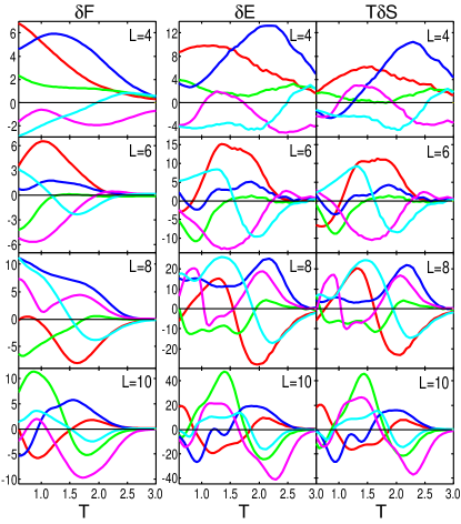
Figure 2: $\delta F$ (left), $\delta E$ (middle) and $T\delta S$ (right) vs. temperature for 5 samples. $L=4,~{}6,~{}8$ and $10$ from top to bottom.

Temperature chaos— In Fig. 2, we show temperature dependence of $\delta F$, $\delta E$ and $T\delta S$ for 5 samples. Oscillations of the three observables become stronger with increasing $L$. We in fact see that $\delta F$ of some samples changes its sign, meaning that the favorable BC with the lower free-energy changes with temperature. We also see that, as predicted by the droplet theory DropletTheory , $\delta E(T)$ and $T\delta S(T)$ exhibit very similar temperature dependence and cancel with each other in the leading order to yield relatively small $\delta F$.

In Fig. 3, the standard deviations, $\sigma_{\rm F}$, $\sigma_{\rm E}$ and $\sigma_{\rm S}$, at $T=0.6J$ are plotted as a function of $L$. Interestingly, $\sigma_{\rm S}$, which gives the amplitude of $|\frac{\partial(\delta F)}{\partial T}|$, increases more rapidly than $\sigma_{\rm F}$, i.e., the amplitude of $\delta F$. See AspelmeierBray02 for a similar observation in the three-dimensional EA model. As argued by Banavar and Bray BanavarBray87 , this result naturally leads us to the conclusion that $\delta F$ in the limit $L\rightarrow\infty$ is totally temperature chaotic.

The inset of Fig. 3 shows $\theta(T)$ and $d_{\rm s}(T)/2$ estimated by linear least-square fits of $\ln(\sigma_{\rm F})$ and $\ln(\sigma_{\rm S})$ against $\ln(L)$ at each temperature. As expected from the droplet theory which is constructed around the $T=0$ fixed point, the two exponents converge to a certain value at low temperatures. By averaging over the lowest five temperatures, we obtain

$$\theta=0.69\pm 0.03,\hskip 14.22636ptd_{\rm s}=3.42\pm 0.06.$$ (3)

Our $\theta$ is compatible with other estimations Hartmann99d ; Hukushima99 , while our $d_{\rm s}$ is somewhat smaller than other ones DSestimation . The apparent temperature dependence of $\theta(T)$ and $d_{\rm s}(T)$ at higher temperatures is considered to be due to the critical fluctuation associated with the unstable fixed point at $T_{\rm c}$, combined with the finite-size effect. Its detailed quantitative analysis is, however, beyond the scope of the present work.

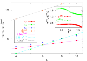
Figure 3: Size dependences of $\sigma_{\rm F}$, $\sigma_{\rm E}$, $\sigma_{\rm S}$ and $\sigma_{\rm S}^{\rm bond}$ at $T=0.6J$. See text for their definitions. The two straight lines for $\sigma_{\rm F}$ and $\sigma_{\rm S}$ are obtained by linear least-square fits of $\ln(\sigma_{\rm F})$/$\ln(\sigma_{\rm S})$ against $\ln(L)$. The line for $\sigma_{\rm S}^{\rm bond}$ has the same slope as that for $\sigma_{\rm S}$. The inset shows the data for $\theta^{\rm(eff)}$ and $d_{\rm s}^{\rm(eff)}/2$.

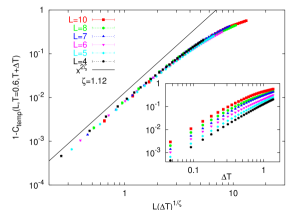
Figure 4: A scaling plot of $1-C_{\rm temp}(L,T,T+\Delta T)$ at $T=0.6J$ against $L(\Delta T)^{1/\zeta}$ with $\zeta=1.12$. The line is proportional to $x^{2\zeta}$. In the inset, $1-C_{\rm temp}$ for $L=4,~{}5,~{}6,~{}7,~{}8$ and $10$ (from bottom to top) are plotted as a function of $\Delta T$.

We next examine the correlation function defined by

$$C_{\rm temp}(L,T,T+\Delta T)\equiv\frac{\overline{\delta F(L,T)\delta F(L,T+\Delta T)}}{\sigma_{\rm F}(L,T)\sigma_{\rm F}(L,T+\Delta T)},$$ (4)

where $\overline{\cdots}$ is the sample average. A similar correlation function was first introduced by Bray and Moore to study bond chaos BrayMoore87 . The inset of Fig. 4 shows the raw data of $1-C_{\rm temp}$ at $T=0.6J$. $C_{\rm temp}$ approaches zero rapidly with increasing $L$. From the prediction of the overlap length by the droplet theory, over which the configurations at the two temperatures are unrelated, we expect one parameter scaling of $C_{\rm temp}=f(L\Delta T^{1/\zeta})$ whose test is shown in the main frame of Fig. 4. We see that the scaling works nicely. The value of $\zeta$ is evaluated to be $1.12\pm 0.05$ by the fitting. Quite interestingly, this value is consistent with the value $\zeta=1.02\pm 0.06$ obtained by substituting eq. (3) into Eq. (1) predicted by the droplet theory. This is one of the main results of the present work. We also see that the data are consistent with the expected asymptotic behavior in the limit $L^{\zeta}\Delta T\rightarrow 0$, $1-C_{\rm temp}\propto(L^{\zeta}\Delta T)^{2}$ BrayMoore87 , as depicted by the line.

Bond chaos and universality— We also study bond chaos by comparing two systems with correlated coupling sets. The perturbed couplings $\{J_{ij}^{\prime}\}$ are obtained from the unperturbed ones $\{J_{ij}\}$ by changing the sign of $J_{ij}$ with probability $p$. Since simulation for bond chaos costs much more time than that for temperature chaos, we only examined $L=4,6,8$ for bond chaos.

Now let us consider an observable $\delta S^{\rm bond}\equiv-\frac{\delta F^{\prime}-\delta F}{\Delta J}$, where $\Delta J\equiv\sqrt{p}$ and $\delta F$ ($\delta F^{\prime}$) is the domain-wall free-energy of the unperturbed (perturbed) system. $\delta S^{\rm bond}$ here and $\delta S$ discussed above are similar in a sense that the both are the increment ratios of $\delta F$ against the perturbations. The ratio against $\Delta J$, not $p$ itself, is considered to compare temperature perturbation and bond perturbation properly Nifle98 . In Fig. 3, the standard deviation of $\delta S^{\rm bond}$, denoted as $\sigma_{\rm S}^{\rm bond}$, is also shown. $\delta S^{\rm bond}$ is estimated with $\Delta J\approx 0.03$, which corresponds to a small value of $p\approx 0.0009$. The line for $\sigma_{\rm S}^{\rm bond}$ and that for $\sigma_{\rm S}$ have the same slope, which suggests that temperature and bond perturbations belong to the same universality class. The coefficient of $\sigma_{\rm S}^{\rm bond}$ is, however, about $16.4$ times as large as that of $\sigma_{\rm S}$. In the inset of Fig. 5 we show the raw data of the correlation function for bond perturbation defined by

$$C_{\rm bond}(L,T,p)\equiv\frac{\overline{\delta F(L,T)\delta F^{\prime}(L,T)}}{\sigma_{\rm F}(L,T)\sigma_{\rm F}^{\prime}(L,T)}.$$ (5)

Again, the correlation decays faster with increasing $L$. In the main frame of Fig. 5, we test a similar scaling to that in Fig. 4 by assuming that the overlap length of the bond perturbation scales as $\Delta J^{-1/\zeta}$. All the data again collapse into a single curve. The chaos exponent $\zeta$ is evaluated to be $1.10\pm 0.10$ by the fitting.

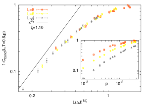
Figure 5: A scaling plot of $1-C_{\rm bond}(L,T,p)$ at $T=0.6J$ against $L(\Delta J)^{1/\zeta}$ with $\zeta=1.10$, where $\Delta J=\sqrt{p}$. The line is proportional to $x^{2\zeta}$. In the inset, the raw data for $L=4,~{}6$ and $8$ (from bottom to top) are shown as a function of $p$.

To compare the two scaling functions for temperature and bond perturbations, we plot in Fig. 6 all the data of both $C_{\rm temp}$ and $C_{\rm bond}$ by using the same chaos exponent. Here we use the value $\zeta=1.12$ in Fig. 4, and multiply the scaling variable $L(\Delta J)^{1/\zeta}$ by factor 17.5. All the data roughly merge into a single curve, indicating that the chaos exponent and the scaling function for temperature chaos are the same as those for bond chaos. Lastly, by estimating the overlap length $\ell$ as the value of $L$ for which $C=0.5$, we obtain

$$\ell_{\rm temp}\approx 11.5\Delta T^{-1/\zeta},\hskip 14.22636pt\ell_{\rm bond}\approx 0.657\Delta J^{-1/\zeta},$$ (6)

where $\zeta\approx 1.12$. We see that the overlap length of the bond perturbation is much shorter than that of the temperature one. This result as well as factor 16.4 in the $\sigma_{\rm S}^{\rm bond}$ scaling mentioned above are the quantitative description of the well-known fact that temperature chaos is much more difficult to be observed than bond chaos Nifle98 ; AspelmeierBray02 .

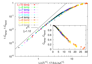
Figure 6: A scaling plot of $1-C$ by using all the data in Figs. 4 and 5. The scaling variable for the data of temperature perturbation is $L(\Delta T)^{1/\zeta}$, while that for the data of bond perturbation is $17.5\times L(\Delta J)^{1/\zeta}$, where $\zeta=1.12$. The line is proportional to $x^{2\zeta}$. The inset shows the same plot for $C$.

Conclusion— In the present work, we have studied the four-dimensional EA Ising spin glass with focus on the chaos effect. As a consequence, many non-trivial predictions by the droplet theory, such as the $\delta F$ oscillation along the temperature axis and the cancellation of $\delta E$ and $T\delta S$ are found in this model. Most importantly, the scaling relation of Eq. (1) and the universal aspect of temperature and bond chaos effects are quantitatively confirmed well inside its spin-glass phase whose thermodynamic properties are dominantly governed by the $T=0$ fixed point. These results are certainly strong evidences for the appropriateness of the droplet theory for the description of chaos effect in the EA Ising spin glasses. On the other hand, recent work by Rizzo and Crisanti RizzoCrisanti02 indicates the existence of similar chaos effects in the Sherrington-Kirkpatrick model. Whether our results are consistent with the mean field view point or not is an interesting open problem.

We would like to thank Dr. Katzgraber for fruitful discussion and useful suggestions. M.S. acknowledges financial support from the Japan Society for the Promotion of Science. The present work is supported by Grant-in-Aid for Scientific Research Program (# 14540351, # 14084204, # 14740233) and NAREGI Nanoscience Project from the MEXT. The present simulations have been performed on SGI 2800/384 at the Supercomputer Center, Institute for Solid State Physics, University of Tokyo.

References

- (1) S. R. McKay, A. N. Berker, and S. Kirkpatrick, Phys. Rev. Lett. 48, 767 (1982).
- (2) H. Kitatani, S. Miyashita and M. Suzuki, J. Phys. Soc. Jpn. 55, 865 (1986).
- (3) F. Ritort, Phys. Rev. B 50, 6844 (1994).
- (4) A. J. Bray and M. A. Moore, Phys. Rev. Lett. 58, 57 (1987).
- (5) M. Ney-Nifle, Phys. Rev. B 57, 492 (1998).
- (6) M. Sales and H. Yoshino, Phys. Rev. E 65, 066131 (2002).
- (7) D. A. Huse and L.-F. Ko, Phys. Rev. B 56, 14597 (1997).
- (8) P. Nordblad and P. Svedlindh, in Spin Glasses and Random Fields, edited by A. P. Young (World Scientific, Singapore, 1998), V. Dupuis et al., Phys. Rev. B 64, 174204 (2001).
- (9) A. Billoire and E. Marinari, J. Phys. A 33, L265 (2000).
- (10) K. Hukushima and Y. Iba, (2002), cond-mat/0207123.
- (11) T. Aspelmeier, A. J. Bray, and M. A. Moore, Phys. Rev. Lett. 89, 197202 (2002).
- (12) A. J. Bray and M. A. Moore, J. Phys. C 17, L463 (1984).
- (13) W. L. McMillan, Phys. Rev. B 31, 340 (1985).
- (14) D. S. Fisher and D. A. Huse, Phys. Rev. Lett. 56, 1601 (1986) and Phys. Rev. B 38, 386 (1988).
- (15) J. R. Banavar and A. J. Bray, Phys. Rev. B 35, 8888 (1987).
- (16) M. Nifle and H. J. Hilhorst, Phys. Rev. Lett 68, 2992 (1992).
- (17) M. Hasenbusch, J. Phys. I France 3, 753 (1993).
- (18) K. Hukushima, Phys. Rev. E 60, 3606 (1999).
- (19) A. K. Hartmann, Phys. Rev. E 60, 5135 (1999).
- (20) K. Hukushima and K. Nemoto, J. Phys. Soc. Jpn. 65, 1604 (1996).
- (21) E. Marinari and F. Zuliani, J. Phys. A 32, 7447 (1999).
- (22) M. Palassini and A. P. Young, Phys. Rev. Lett. 85, 3017 (2000); H. G. Katzgraber, M. Palassini and A. P. Young, Phys. Rev. B 63, 184422 (2001).
- (23) T. Rizzo and A. Crisanti, Phys. Rev. Lett. 90, 137201 (2003).